What Kind of Language Is Hard to Language Model?

(1)

4975

What Kind of Language Is Hard to Language-Model?

Sebastian J. Mielke1 Ryan Cotterell1 Kyle Gorman2,3 Brian Roark3 Jason Eisner1

1_{Department of Computer Science, Johns Hopkins University}

2_{Program in Linguistics, Graduate Center, City University of New York} 3_Google

{sjmielke@,ryan.cotterell@}jhu.edu [email protected]

[email protected] [email protected]

Abstract

How language-agnostic are current state-of-the-art NLP tools? Are there some types of language that are easier to model with cur-rent methods? In prior work (Cotterell et al.,

2018) we attempted to address this question for language modeling, and observed that re-current neural network language models do not perform equally well over all the high-resource European languages found in the Europarl corpus. We speculated that inflec-tional morphology may be the primary cul-prit for the discrepancy. In this paper, we ex-tend these earlier experiments to cover 69 lan-guages from 13 language families using a mul-tilingual Bible corpus. Methodologically, we introduce a new paired-sample multiplicative mixed-effects model to obtain language dif-ficulty coefficients from at-least-pairwise par-allel corpora. In other words, the model is aware of inter-sentence variation and can han-dle missing data. Exploiting this model, we show that “translationese” is not any easier to model than natively written language in a fair comparison. Trying to answer the question of what features difficult languages have in com-mon, we try and fail to reproduce our earlier (Cotterell et al.,2018) observation about mor-phological complexity and instead reveal far simpler statistics of the data that seem to drive complexity in a much larger sample.

1 Introduction

Do current NLP tools serve all languages? Tech-nically, yes, as there are rarely hard constraints that prohibit application to specific languages, as long as there is data annotated for the task. However, in practice, the answer is more nuanced: as most studies seem to (unfairly) assume English is representative of the world’s languages (Bender,

2009), we do not have a clear idea how well models perform cross-linguistically in a controlled setting. In this work, we look at current methods for lan-guage modeling and attempt to determine whether

Resump-tion of the session

Wieder- aufnah-me der ... The peace that ...

Der gestern verein-...

Мирът, който беше ... Obwohl wir nicht ...

Макар че не бяхме ... Now we

can fi-nally ...

Накрая всички можем ...

en de bg

1

2

3

4

aligned multi-text

language

model

y1,en y1,de

y2,en y2,de y2,bg

y3,de y3,bg

y4,en y4,bg

Difficulty estimation from sentence surprisal

n1

n2

n3

n4

⇒

den dde dbg

[image:1.595.310.527.205.342.2]

⇒ ⇒ ⇒

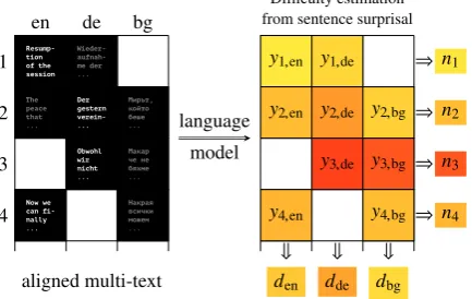
Figure 1: Jointly estimating the informationnipresent

in each multi-text intenti andthe difficultydj of each

language j. At left, gray text indicates translations of the original (white) sentence in the same row. At right, darker cells indicate higher surprisal/difficulty. Empty cells indicate missing translations. English (en) is miss-ing a hard sentence and Bulgarian (bg) is missmiss-ing an easy sentence, but this does not mislead our method into estimating English as easier than Bulgarian.

there are typological properties that make certain languages harder to language-model than others.

One of the oldest tasks in NLP (Shannon,1951) is language modeling, which attempts to estimate a distribution p(x) over strings x of a language. Recent years have seen impressive improvements with recurrent neural language models (e.g.,Merity et al.,2018). Language modeling is an important component of tasks such as speech recognition, ma-chine translation, and text normalization. It has also enabled the construction of contextual word embed-dings that provide impressive performance gains in many other NLP tasks (Peters et al.,2018)—though those downstream evaluations, too, have focused on a small number of (mostly English) datasets.

(2)

use of the Europarl corpus which, unfortunately, is not very typologically diverse. Using a corpus with relatively few (and often related) languages limits the kinds of conclusions that can be drawn from any resulting comparisons. In this paper, we present an alternative method that does not require the corpus to befullyparallel, so that collections consisting of many more languages can be com-pared. Empirically, we report language-modeling results on 62 languages from 13 language families using Bible translations, and on the 21 languages used in the European Parliament proceedings.

We suppose that a language model’s surprisal on a sentence—the negated log of the probability it as-signs to the sentence—reflects not only the length and complexity of the specific sentence, but also the general difficulty that the model has in predict-ing sentences of that language. Given language models of diverse languages, we jointly recover each language’s difficulty parameter. Our regres-sion formula explains the variance in the dataset better than previous approaches and can also deal with missing translations for some purposes.

Given these difficulty estimates, we conduct a correlational study, asking which typological fea-tures of a language are predictive of modeling diffi-culty. Our results suggest that simple properties of a language—the word inventory and (to a lesser ex-tent) the raw character sequence length—are statis-tically significant indicators of modeling difficulty within our large set of languages. In contrast, we fail to reproduce our earlier results fromCotterell et al.(2018),1which suggested morphological com-plexity as an indicator of modeling comcom-plexity. In fact, we find no tenable correlation to a wide vari-ety of typological features, taken from the WALS dataset and other sources. Additionally, exploiting our model’s ability to handle missing data, we di-rectly test the hypothesis that translationese leads to easier language-modeling (Baker,1993; Lem-bersky et al.,2012). We ultimately cast doubt on this claim, showing that, under the strictest con-trols, translationese isdifferent, but not anyeasier

to model according to our notion of difficulty. We conclude with a recommendation: The world

1_{We can certainly}_replicate_{those results in the sense that,}

using the surprisals from those experiments, we achieve the same correlations. However, we did notreproducethe results under new conditions (Drummond,2009). Our new conditions included a larger set of languages, a more sophisticated diffi-culty estimation method, and—perhaps crucially—improved language modeling families that tend to achieve better sur-prisals (or equivalently, better perplexity).

being small, typology is in practice a small-data problem. there is a real danger that cross-linguistic studies will under-sample and thus over-extrapolate. We outline directions for future, more robust, investigations, and further caution that future work of this sort should focus on datasets with far more languages, something our new methods now allow.

2 The Surprisal of a Sentence

When trying to estimate the difficulty (or complex-ity) of a language, we face a problem: the predic-tiveness of a language model on a domain of text will reflect not only the language that the text is written in, but also the topic, meaning, style, and in-formation density of the text. To measure the effect due only to the language, we would like to compare on datasets that are matched for the other variables, to the extent possible. The datasets should all con-tain the same content, the only difference being the language in which it is expressed.

2.1 Multitext for a Fair Comparison

To attempt a fair comparison, we make use of mul-titext—sentence-aligned2translations of thesame

contentin multiple languages. Different surprisals

on the translations of the same sentence reflect qual-ity differences in the language models, unless the translators added or removed information.3

In what follows, we will distinguish between the

ithsentencein languagej, which is a specific string

si j, and theith intent, the shared abstract thought that gave rise to all the sentences s_i₁,s_i₂, . . .. For simplicity, suppose for now that we have a fully parallel corpus. We select, say, 80% of the intents.4 We use the English sentences that express these intents to train an English language model, and test it on the sentences that express the remaining 20% of the intents. We will later drop the assumption of a fully parallel corpus (§3), which will help us to estimate the effects of translationese (§6).

2_{Both corpora we use align small paragraphs instead of}

sentences, but for simplicity we will call them “sentences.”

3_{A translator might add or remove information out of}

help-fulness, sloppiness, showiness, consideration for their audi-ence’s background knowledge, or deference to the conventions of the target language. For example, English conventions make it almost obligatory to express number (via morphological in-flection), but make it optional to express evidentiality (e.g., via an explicit modal construction); other languages are different.

4_{In practice, we use}₂_/₃_{of the raw data to train our models,}

(3)

2.2 Comparing Surprisal Across Languages

Given some test sentencesi j, a language modelp defines itssurprisal: the negative log-likelihood

NLL(si j)=−log2p(si j). This can be interpreted as the number of bits needed to represent the sen-tence under a compression scheme that is derived from the language model, with high-probability sentences requiring the fewest bits. Long or un-usual sentences tend to have high surprisal—but high surprisal can also reflect a language’s model’s

failure to anticipate predictable words. In fact,

language models for the same language are often comparatively evaluated by theiraverage surprisal

on a corpus (the cross-entropy). Cotterell et al.

(2018) similarly compared language models for different languages, using a multitext corpus.

Concretely, recall thats_{i j}ands_{i j}0should contain,

at least in principle, the same information for two languages jand j0—they are translations of each other. But, if we find thatNLL(s_{i j}) > NLL(s_{i j}0),

we must assume that eithersi j contains more infor-mation thans_{i j}0, or that our language model was

simply able to predict it less well.5 If we were to assume that our language models were perfect in the sense that they captured the true probability dis-tribution of a language, we could make the former claim; but we suspect that much of the difference can be explained by our imperfect LMs rather than inherent differences in the expressed information (see the discussion in footnote3).

2.3 Our Language Models

Specifically, the crude tools we use are recurrent neural network language models (RNNLMs) over different types of subword units. For fairness, it is of utmost importance that these language models areopen-vocabulary, i.e., they predict the entire string and cannot cheat by predicting only UNK (“unknown”) for some words of the language.6

Char-RNNLM The first open-vocabulary

RNNLM is the one of Sutskever et al. (2011), whose model generates a sentence, not word by

5_{The former might be the result of overt marking of, say,}

evidentiality or gender, which adds information. We hope that these differences are taken care of by diligent translators producing faithful translations in our multitext corpus.

6_{We restrict the set of characters to those that we see at}

least 25 times in the training set, replacing all others with a new symbol^, as is common and easily defensible in

open-vocabulary language modeling (Mielke and Eisner,2018). We make an exception for Chinese, where we only require each character to appear at least twice. These thresholds result in negligible “out-of-alphabet” rates for all languages.

word, but rather character by character. An obvious drawback of the model is that it has no explicit representation of reusable substrings (Mielke and Eisner, 2018), but the fact that it does not rely on a somewhat arbitrary word segmentation or tokenization makes it attractive for this study. We use a more current version based on LSTMs (Hochreiter and Schmidhuber, 1997), using the implementation of Merity et al. (2018) with the char-PTB parameters.

BPE-RNNLM BPE-based open-vocabulary

lan-guage models make use of sub-word units instead of either words or characters and are a strong base-line on multiple languages (Mielke and Eisner,

2018). Before training the RNN,byte pair encod-ing(BPE;Sennrich et al.,2016) is applied globally to the training corpus, splitting each word (i.e., each space-separated substring) into one or more units. The RNN is then trained over the sequence of units, which looks like this: “The |ex|os|kel|eton |is

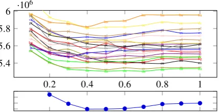
|gener|ally |blue”. The set of subword units is fi-nite and determined from training data only, but it is a superset of the alphabet, making it possible to explain any novel word in held-out data via some segmentation.7 One important thing to note is that the size of this set can be tuned by specifying the number of BPEmerges, allowing us to smoothly vary between a word-level model (∞merges) and a kind of character-level model (0 merges). As Figure2shows, the number of merges that max-imizes log-likelihood of our dev set differs from language to language.8 However, as we will see in Figure3, tuning this parameter does not substan-tially influence our results. We therefore will refer to the model with0.4|V|merges as BPE-RNNLM.

3 Aggregating Sentence Surprisals

Cotterell et al.(2018) evaluated the model for lan-guage jsimply by its total surprisalP

iNLL(si j). This comparative measure required a complete mul-titext corpus containing every sentencesi j(the ex-pression of the intenti in language j). We relax this requirement by using a fully probabilistic re-gression model that can deal with missing data

7_{In practice, in both training and testing, we only evaluate}

the probability of the canonical segmentation of the held-out string, rather than the total probability of all segmentations (Kudo,2018;Mielke and Eisner,2018, Appendix D.2).

8_Figure₂_{shows the 21 languages of the Europarl dataset.}

(4)

0.2 0.4 0.6 0.8 1 5.4 5.6 5.8 6 ·10 6 bg bg bg

bg bg bg bg bg bg bg

cs cs

cs cs cs cs

da

da da da da da da da da

de de

de de de de de de de el

el el

el el el el el el el

en

en en

en

en en en en en en

es

es es es es es _es es es

et

et et et

et et et et et et

fi

fi fi

fi fi fi fi fi

fr

fr fr fr

fr fr fr fr fr fr

hu

hu hu hu

hu hu

hu hu hu hu

it it it it it it

it it it it

lt lt

lt lt lt lt lt lt

lv

lv lv lv lv lv

lv lv lv

nl

nl _nl nl nl

nl nl nl nl pl

pl pl

pl pl pl pl

pl pl pl

pt

pt pt

pt _pt

pt pt pt pt pt

ro

ro ro

ro ro ro

ro ro

sk

sk _sk _sk sk sk sk sk sk

sl

sl _sl

sl sl sl sl sl sl sl

sv sv

[image:4.595.76.291.57.167.2]

sv sv _sv sv sv sv sv sv

Figure 2: Top: For each language, total NLL of the dev corpus varies with the number of BPE merges, which is expressed on the x-axis as a fraction of the number of observed word types |V|.8 _{Bottom: Averaging over}

all 21 languages motivates a global value of 0.4.

(Figure1).9 Our model predicts each sentence’s surprisal yi j = NLL(si j) using an intent-specific “information content” factorni, which captures the inherent surprisal of the intent, combined with a language-specific difficulty factor d_j. This repre-sents a better approach to varying sentence lengths and lets us work with missing translations in the test data (though it does not remedy our need for fully parallel language model training data).

3.1 Model 1: Multiplicative Mixed-effects

Model 1 is a multiplicative mixed-effects model:

yi j =ni·exp(dj)·exp(i j) (1)

i j ∼N(0, σ2) (2)

This says that each intentihas a latentsizeofni— measured in some abstract “informational units”— that is observed indirectly in the various sentences

si j that express the intent. Larger ni tend to yield longer sentences. Sentence si j has yi j bits of surprisal; thus the multiplier yi j/ni represents

the number of bits that language j used to ex-press each informational unit of intent i, under our language model of language j. Our mixed-effects model assumes that this multiplier is log-normally distributed over the sentencesi: that is,

log(yi j/ni) ∼N(dj, σ2), where meandjis the

dif-ficultyof languagej. That is,yi j/_n_i =exp(d_j+_{i j})

wherei j ∼ N(0, σ2) is residual noise, yielding equations (1)–(2).10We jointly fit the intent sizes

niand the language difficultiesdj.

9_{Specifically, we deal with data missing completely at}

random (MCAR), a strong assumption on the data generation process. More discussion on this can be found in AppendixA.

10_{It is tempting to give each language its own}_σ2

j

parame-ter, but then the MAP estimate is pathological, since infinite likelihood can be attained by setting one language’sσ2_j to 0.

3.2 Model 2: Heteroscedasticity

Because it is multiplicative, Model 1 appropriately predicts that in each language j, intents with large

n_i will not only have larger yi j values but these values will vary more widely. However, Model 1 is homoscedastic: the varianceσ2 of log(yi j/ni)

is assumed to be independent of the independent variableni, which predicts that the distribution of yi j should spread outlinearlyas the information contentn_iincreases: e.g.,p(yi j ≥ 13| ni =10)=

p(yi j ≥ 26 | ni = 20). That assumption is ques-tionable, since for a longer sentence, we would ex-pectlogyi j/ni to come closer to its meandjas the random effects of individual translational choices average out.11 We address this issue by assuming thatyi jresults fromni ∈Nindependent choices:

yi j =exp(dj)·*

, ni X

k=1

expi jk+

-(3)

i jk ∼N(0, σ2) (4)

The number of bits for thekth informational unit now varies by a factor ofexpi jkthat is log-normal and independent of the other units. It is common to approximate the sum of independent log-normals by another log-normal distribution, matching mean and variance (Fenton-Wilkinson approximation;

Fenton,1960),12yielding Model 2:

yi j =ni·exp(dj)·exp(i j) (1)

σ2 i =ln

1+ exp(σ_n2)−1

i

(5)

i j ∼N

σ2−σ2_i

2 , σ 2 i

, (6)

in which the noise term i j now depends on ni. Unlike (4), this formula no longer requiresni ∈N; we allow anyn_i ∈R>0, which will also let us use gradient descent in estimatingni.

In effect, fitting the model chooses each ni so that the resulting intent-specific but language-independent distribution ofni·exp(i j) values,13

11_{Similarly, flipping a fair coin 10 times results in} ₅_±

1.58heads where 1.58 represents the standard deviation, but flipping it 20 times does not result in10±1.58·2heads but rather10±1.58·

√

2heads. Thus, with more flips, the ratio heads/flips tends to fall closer to its mean 0.5.

12_{There are better approximations, but even the only slightly}

more complicated Schwartz-Yeh approximation (Schwartz and Yeh,1982) already requires costly and complicated ap-proximations in addition to lacking the generalizability to non-integralnivalues that we will obtain for the Fenton-Wilkinson approximation.

13_{The distribution of}

i jis the same for everyj. It no longer

(5)

after it is scaled by exp(dj) for each language j, will assign high probability to the observed yi j. Notice that in Model 2, the scale of ni becomes meaningful: fitting the model will choose the size of the abstract informational units so as to predict how rapidlyσifalls off withni. This contrasts with Model 1, where doubling all then_ivalues could be compensated for by halving all theexp(dj) values.

3.3 Model 2L: An Outlier-Resistant Variant

One way to make Model 2 more outlier-resistant is to use a Laplace distribution14instead of a Gaus-sian in (6) as an approximation to the distribution ofi j. The Laplace distribution is heavy-tailed, so it is more tolerant of large residuals. We choose its mean and variance just as in (6). This heavy-tailed

i j distribution can be viewed as approximating a version of Model 2 in which thei jk themselves follow some heavy-tailed distribution.

3.4 Estimating model parameters

We fit each regression model’s parameters by L-BFGS. We then evaluate the model’s fitness by measuring its held-out data likelihood—that is, the probability it assigns to the yi jvalues for held-out intentsi. Here we use the previously fitteddjand

σparameters, but we must newly fitn_ivalues for the newiusing MAP estimates or posterior means. A full comparison of our models under various con-ditions can be found in AppendixC. The primary findings are as follows. On Europarl data (which has fewer languages), Model 2 performs best. On the Bible corpora, all models are relatively close to one another, though the robust Model 2L gets more consistent results than Model 2 across data sub-sets. We use MAP estimates under Model 2 for all remaining experiments for speed and simplicity.15

3.5 A Note on Bayesian Inference

As our model ofyi jvalues is fully generative, one could place priors on our parameters and do full inference of the posterior rather than performing MAP inference. We did experiment with priors but found them so quickly overruled by the data that it did not make much sense to spend time on them.

Specifically, for full inference, we implemented all models in STAN (Carpenter et al., 2017), a

14_{One could also use a Cauchy distribution instead of the}

Laplace distribution to get even heavier tails, but we saw little difference between the two in practice.

15_{Further enhancements are possible: we discuss our}

“Model 3” in AppendixB, but it did not seem to fit better.

toolkit for fast, state-of-the-art inference using Hamiltonian Monte Carlo (HMC) estimation. Run-ning HMC unfortunately scales sublinearly with the number of sentences (and thus results in very long sampling times), and the posteriors we ob-tained were unimodal with relatively small vari-ances (see also AppendixC). We therefore work with the MAP estimates in the rest of this paper.

4 The Difficulties of 69 languages

Having outlined our method for estimating language difficulty scoresdj, we now seek data to do so for all our languages. If we wanted to cover the most languages possible with parallel text, we should surely look at the Universal Declaration of Human Rights, which has been translated into over 500 languages. Yet this short document is far too small to train state-of-the-art language models. In this paper, we will therefore follow previous work in using the Europarl corpus (Koehn, 2005), but also for the first time make use of 106 Bibles from

Mayer and Cysouw(2014)’s corpus.

Although our regression models of the surprisals yi j can be estimated from incomplete multitext, the surprisals themselves are derived from the lan-guage models we are comparing. To ensure that the language models are comparable, we want to train them on completely parallel data in the various languages. For this, we seek complete multitext.

4.1 Europarl: 21 Languages

The Europarl corpus (Koehn, 2005) contains decades worth of discussions of the European Par-liament, where each intent appears in up to 21 lan-guages. It was previously used byCotterell et al.

(2018) for its size and stability. In§6, we will also exploit the fact that each intent’s original language is known. To simplify our access to this infor-mation, we will use the “Corrected & Structured Europarl Corpus” (CoStEP) corpus (Gra¨en et al.,

2014). From it, we extract the intents that appear in all 21 languages, as enumerated in footnote8. The full extraction process and corpus statistics are detailed in AppendixD.

4.2 The Bible: 62 Languages

The Bible is a religious text that has been used for decades as a dataset for massively multilin-gual NLP (Resnik et al., 1999; Yarowsky et al.,

(6)

chars

BPE (0.4|V|)

BPE (best per language)

bg cs

da el de

en lt it fi es et hu fr

[image:6.595.77.286.57.113.2]

lv sl sk sv ro nl pt pl

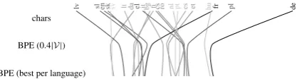
Figure 3: The Europarl language difficulties appear more similar, and are ordered differently, when the RNN models use BPE units instead of character units. Tuning BPE per-language has a small additional effect.

tokenized16 and aligned collection assembled by

Mayer and Cysouw(2014). We use the smallest annotated subdivision (a singleverse) as a sentence in our difficulty estimation model; see footnote2.

Some of the Bibles in the dataset are incomplete. As the Bibles include different sets of verses (in-tents), we have to select a set of Bibles that overlap strongly, so we can use the verses shared by all these Bibles to comparably train all our language models (and fairly test them: see Appendix A). We cast this selection problem as an integer lin-ear program (ILP), which we solve exactly in a few hours using the Gurobi solver (more details on this selection in AppendixE). This optimal so-lution keeps 25996 verses, each of which appears across 106 Bibles in 62 languages,17spanning 13 language families.18 We allow jto range over the 106 Bibles, so when a language has multiple Bibles, we estimate a separate difficultydj for each one.

4.3 Results

The estimated difficulties are visualized in Figure4. We can see that general trends are preserved be-tween datasets: German and Hungarian are hardest, English and Lithuanian easiest. As we can see in Figure3for Europarl, the difficulty estimates are

16_{The fact that the resource is tokenized is (yet) another}

possible confound for this study: we are not comparing per-formance on languages, but on languages/Bibleswith some specific translator and tokenization. It is possible that ouryi j

values for each language jdepend to a small degree on the tokenizer that was chosen for that language.

17_{afr, aln, arb, arz, ayr, bba, ben, bqc, bul, cac, cak, ceb, ces,}

cmn, cnh, cym, dan, deu, ell, eng, epo, fin, fra, guj, gur, hat, hrv, hun, ind, ita, kek, kjb, lat, lit, mah, mam, mri, mya, nld, nor, plt, poh, por, qub, quh, quy, quz, ron, rus, som, tbz, tcw, tgl, tlh, tpi, tpm, ukr, vie, wal, wbm, xho, zom

18_{22 Indo-European, 6 Niger-Congo, 6 Mayan, 6}

Austrone-sian, 4 Sino-Tibetan, 4 Quechuan, 4 Afro-Asiatic, 2 Uralic, 2 Creoles, 2 Constructed languages, 2 Austro-Asiatic, 1 To-tonacan, 1 Aymaran. For each language, we are reporting here the first family listed by Ethnologue (Paul et al.,2009), manually fixing tlh7→Constructed language. It is unfortunate not to have more families or more languages per family. A broader sample could be obtained by taking only the New Testament—but unfortunately that has<8000verses, a mea-ger third of our dataset that is already smaller that the usually considered tiny PTB dataset (see details in AppendixE).

hardly affected when tuning the number of BPE merges per-language instead of globally, validat-ing our approach of usvalidat-ing the BPE model for our experiments. A bigger difference seems to be the choice of char-RNNLM vs. BPE-RNNLM, which changes the ranking of languages both on Europarl data and on Bibles. We still see German as the hardest language, but almost all other languages switch places. Specifically, we can see that the variance of the char-RNNLM is much higher.

4.4 Are All Translations the Same?

Texts like the Bible are justly infamous for their sometimes archaic or unrepresentative use of lan-guage. The fact that we sometimes have multiple Bible translations in the same language lets us ob-serve variation by translation style.

The sample standard deviation ofdj among the 106 Bibles jis 0.076/0.063 for BPE/char-RNNLM. Within the 11 German, 11 French, and 4 En-glish Bibles, the sample standard deviations were roughly 0.05/0.04, 0.05/0.04, and 0.02/0.04 respec-tively: so style accounts for less than half the vari-ance. We also consider another parallel corpus, created from the NIST OpenMT competitions on machine translation, in which each sentence has 4 English translations (NIST Multimodal Informa-tion Group,2010a,b,c,d,e,f,g,2013b,a). We get a sample standard deviation of 0.01/0.03 among the 4 resulting English corpora, suggesting that language difficulty estimates (particularly the BPE estimate) depend less on the translator, to the extent that these corpora represent individual translators.

5 What Correlates with Difficulty?

Making use of our results on these languages, we can now answer the question: what features of a language correlate with the difference in language complexity? Sadly, we cannot conduct all analyses on all data: the Europarl languages are well-served by existing tools like UDPipe (Straka et al.,2016), but the languages of our Bibles are often not. We therefore conduct analyses that rely on automati-cally extracted features only on the Europarl cor-pora. Note that to ensure a false discovery rate of at mostα = .05, all reportedp-values have to be corrected usingBenjamini and Hochberg(1995)’s procedure: onlyp≤ .05·5/₂₈_≈₀.₀₀₉_{is significant.}

Morphological Counting Complexity

(7)

−4 −3 −2 −1 0 1 2 3 4 5 −8 −6 −4 −2 0 2 4 6 8 10

easier with BPE

easier with chars

bg cs da de el en eset fi fr hu it lt lv nl pl pt ro sk sl sv

difficulty (×100) using BPE-RNNLM with 0.4|V|merges

dif ficulty ( × 100 ) using char -RNNLM

Difficulties on Europarl vs.

harder easier bg cs da de el en fi fr hu it lt nl pt ro bul ces dan deu ell eng fin fra hun ita lit nld por ron

−15 −10 −5 0 5 10 15 20 25

−15 −10 −5 0 5 10 15 20

easier with BPE

easier with chars afr aln arb arz ayr ayr bba ben ben bqc bul bul cac cak

cebcebceb

ces ces cmn cnh cymdan deu deu deu deu deu deu deu deu deu deu deu ell eng eng eng eng epo fin fin fin frafra fra fra fra fra fra fra fra fra fra guj gur hat hat hrv hun hun ind ind ita ita ita ita kek kek kjb lat lit mah mammri mya nld nor nor plt poh por por por qub quh quy quz ron rus som tbz tcw tgl tlh tpi tpm ukrukr vie vie vie wal wbm xho zom

difficulty (×100) using BPE-RNNLM with 0.4|V|merges

dif ficulty ( × 100 ) using char -RNNLM

[image:7.595.77.522.57.254.2]

Difficulties on Bibles

Figure 4: Difficulties of 21 Europarl languages (left) and 106 Bibles (right), comparing difficulties when estimated from BPE-RNNLMs vs. char-RNNLMs. Highlighted on the right are deu and fra, for which we have many Bibles, and eng, which has often been prioritized even over these two in research. In the middle we see the difficulties of the 14 languages that are shared between the Bibles and Europarl aligned to each other (averaging all estimates), indicating that the general trends we see are not tied to either corpus.

choose among forms like “talk,” “talks,” “talking”) was mainly responsible for difficulty in modeling. They found a language’s Morphological Counting Complexity (Sagot,2013) to correlate positively with its difficulty. We use the reported MCC values from that paper for our 21 Europarl languages, but to our surprise, find no statistically significant correlation with the newly estimated difficulties of our new language models. Comparing the scatterplot for both languages in Figure 5 with

Cotterell et al.(2018)’s Figure 1, we see that the high-MCC outlier Finnish has become much easier in our (presumably) better-tuned models. We suspect that the reported correlation in that paper was mainly driven by such outliers and conclude that MCC is not a good predictor of modeling difficulty. Perhaps finer measures of morphological complexity would be more predictive.

Head-POS Entropy Dehouck and Denis(2018) propose an alternative measure of morphosyntactic complexity. Given a corpus of dependency graphs, they estimate the conditional entropy of the POS tag of a random token’s parent, conditioned on the token’s type. In a language where thisHPE-mean

metric is low, most tokens can predict the POS of their parent even without context. We compute HPE-mean from dependency parses of the Europarl data, generated using UDPipe 1.2.0 (Straka et al.,

2016) and freely-available tokenization, tagging, parsing models trained on the Universal Depen-dencies 2.0 treebanks (Straka and Strakov,2017).

HPE-mean may be regarded as the mean over all corpus tokens ofHead POS Entropy(Dehouck and Denis,2018), which is the entropy of the POS tag of a token’s parent given thatparticulartoken’s type. We also computeHPE-skew, the (positive) skewness of the empirical distribution of HPE on the corpus tokens. We remark that in each language, HPE is 0 for most tokens.

As predictors of language difficulty, HPE-mean has a Spearman’s ρ = .004/−.045 (p > .9/.8) and HPE-skew has a Spearman’s ρ = .032/.158

(p> .8/.4), so this is not a positive result.

Average dependency length It has been

ob-served that languages tend to minimize the distance between heads and dependents (Liu,2008). Speak-ers prefer shorter dependencies in both production and processing, and average dependency lengths tend to be much shorter than would be expected from randomly-generated parses (Futrell et al.,

2015;Liu et al.,2017). On the other hand, there is substantial variability between languages, and it has been proposed, for example, that head-final languages and case-marking languages tend to have longer dependencies on average.

(8)

0 50 100 150 200

−4

−2 0 2 4

bg

cs

da de

el

en

et

fi fr

hu

it

lv lt nl

pl

pt ro

sk sl

es

sv

MCC

dif

ficulty

(

×

100

,

BPE-RNNLM)

0 50 100 150 200

−5 0 5 10

bg cs

da de

el

en

et

fi

fr hu

it

lv lt nl

pl

pt

ro

sk sl es

sv

MCC

dif

ficulty

(

×

100

,

char

[image:8.595.72.291.54.170.2]

-RNNLM)

Figure 5: MCC does not predict difficulty on Europarl. Spearman’s ρ is .091 / .110 with p > .6 for BPE-RNNLM (left) / char-BPE-RNNLM (right).

which excludes punctuation and standardizes sev-eral other grammatical relationships (e.g., objects of prepositions are made to depend on their prepo-sitions, and verbs to depend on their complemen-tizers). Our hypothesis that scrambling makes language harder to model seems confirmed at first: while the non-parametric (and thus more weakly powered) Spearman’s ρ = .196/.092

(p = .394/.691), Pearson’s r = .486/.522(p =

.032/.015). However, after correcting for multiple comparisons, this is also non-significant.19

WALS features The World Atlas of Language

Structures (WALS;Dryer and Haspelmath,2013) contains nearly 200 binary and integer features for over 2000 languages. Similarly to the Bible situation, not all features are present for all languages—and for some of our Bibles, no infor-mation can be found at all. We therefore restrict our attention to two well-annotated WALS features that are present in enough of our Bible languages (fore-going Europarl to keep the analysis simple): 26A “Prefixing vs. Suffixing in Inflectional Morphology”

and 81A “Order of Subject, Object and Verb.” The results are again not quite as striking as we would hope. In particular, in Mood’s median null hypothesis significance test neither 26A (p > .3

/ .7 for BPE/char-RNNLM) nor 81A (p > .6 /

.2 for BPE/char-RNNLM) show any significant differences between categories (detailed results in AppendixF.1). We therefore turn our attention to much simpler, yet strikingly effective heuristics.

Raw character sequence length An interesting correlation emerges between language difficulty

19_{We also caution that the significance test for Pearson’s}

assumes that the two variables are bivariate normal. If not, then even a significantrdoes not allow us to reject the null hypothesis of zero covariance (Kowalski,1972, Figs. 1–2,§5).

for the RNNLM and the raw length in char-acters of the test corpus (detailed results in Ap-pendix F.2). On both Europarl and the more re-liable Bible corpus, we have positive correlation for the char-RNNLM at a significance level of

p< .001, passing the multiple-test correction. The BPE-RNNLM correlation on the Bible corpus is very weak, suggesting that allowing larger units of prediction effectively eliminates this source of difficulty (van Merri¨enboer et al.,2017).

Raw word inventory Our most predictive fea-ture, however, is thesize of the word inventory. To obtain this number, we count the number of distinct types |V| in the (tokenized) training set of a lan-guage (detailed results in AppendixF.3).20 While again there is little power in the small set of Eu-roparl languages, on the bigger set of Bibles we do see the biggest positive correlation of any of our features—but only on the BPE model (p<1e−11). Recall that the char-RNNLM has no notion of words, whereas the number of BPE units increases with|V|(indeed, many whole words are BPE units, because we do many merges but BPE stops at word boundaries). Thus, one interpretation is that the Bible corpora are too small to fit the parameters for all the units needed in large-vocabulary lan-guages. A similarly predictive feature on Bibles— whose numerator is this word inventory size—is the type/token ratio, where values closer to 1 are a traditional omen of undertraining.

An interesting observation is that on Europarl, the size of the word inventory and the morpholog-ical counting complexity of a language correlate quite well with each other (Pearson’s ρ=.693at

p=.0005, Spearman’s ρ= .666atp=.0009), so the original claim inCotterell et al.(2018) about MCC may very well hold true after all. Unfor-tunately, we cannot estimate the MCC for all the Bible languages, or this would be easy to check.21 Given more nuanced linguistic measures (or more languages), our methods may permit discov-ery of specific linguistic correlates of modeling difficulty, beyond these simply suggestive results.

20_{A more sophisticated version of this feature might}

con-sider not just the existence of certain forms but also their rates of appearance. We did calculate the entropy of the unigram distribution over words in a language, but we found that is strongly correlated with the size of the word inventory and not any more predictive.

21_{Perhaps in a future where more data has been annotated}

(9)

6 Evaluating Translationese

Our previous experiments treat translated sentences just like natively generated sentences. But since Europarl contains information about which lan-guage an intent was originally expressed in,22here we have the opportunity to ask another question: is translationese harder, easier, indistinguishable, or impossible to tell? We tackle this question by splitting each language jinto two sub-languages, “native” jand “translated” j, resulting in 42 sub-languages with 42 difficulties.23 Each intent is expressed in at most 21 sub-languages, so this ap-proachrequiresa regresssion method that can han-dle missing data, such as the probabilistic approach we proposed in§3. Our mixed-effects modeling ensures that our estimation focuses on the differ-ences between languages, controlling for content by automatically fitting the ni factors. Thus, we are not in danger of calling native German more complicated than translated German just because German speakers in Parliament may like to talk about complicated things in complicated ways.

In a first attempt, we simply use our already-trained BPE-best models (as they perform the best and are thus most likely to support claims about the language itself rather than the shortcomings of any singular model), limit ourselves to only splitting the eight languages that have at least 500 native sentences24 (to ensure stable results). Indeed we

seemto find that native sentences are slightly more difficult: theirdjis 0.027 larger (±0.023, averaged over our selected 8 languages).

But are they? This result is confounded by the fact that our RNN language modelswere trained

mostly on translationese text (even the English data is mostly translationese). Thus, translationese might merely bedifferent(Rabinovich and Wintner,

2015)—not necessarily easier to model, but over-represented when training the model, making the translationese test sentences more predictable. To remove this confound, we must train our language

22_{It should be said that using Europarl for translationese}

studies is not without caveats (Rabinovich et al.,2016), one of them being the fact that not all language pairs are translated equally: a natively Finnish sentence is translated first into English, French, or German (pivoting) and only from there into any other language like Bulgarian.

23_{This method would also allow us to study the effect of}

source language, yieldingdj←j0for sentences translated from

j0intoj. Similarly, we could have included surprisals from

bothmodels,jointlyestimatingdj,char-RNNanddj,BPEvalues. 24_{en (3256), fr (1650), de (1275), pt (1077), it (892), es}

(685), ro (661), pl (594)

models on equal parts translationese and native text. We cannot do this for multiple languages at once, given our requirement of training all language mod-els on the same intents. We thus choose to balance onlyonelanguage—we train all models for all lan-guages, making sure that the training set for one language is balanced—and then perform our regres-sion, reporting the translationese and native difficul-ties only for the balanced language. We repeat this process for every language that has enough intents. We sample equal numbers of native and non-native sentences, such that there are∼1M words in the corresponding English column (to be comparable to the PTB size). To raise the number of languages we can split in this way, we restrict ourselves here to fully-parallel Europarl in only 10 languages25 instead of 21, thus ensuring that each of these 10 languages has enough native sentences.

On this level playing field, the previously ob-served effect practically disappears (-0.0044 ±

0.022), leading us to question the widespread hy-pothesis that translationese is “easier” to model (Baker,1993).26

7 Conclusion

There is a real danger in cross-linguistic studies of over-extrapolating from limited data. We re-evaluated the conclusions ofCotterell et al.(2018) on a larger set of languages, requiring new methods to select fully parallel data (§4.2) or handle missing data. We showed how to fit a paired-sample multi-plicative mixed-effects model to probabilistically obtain language difficulties from at-least-pairwise parallel corpora. Our language difficulty estimates were largely stable across datasets and language model architectures, but they were not significantly predicted by linguistic factors. However, a lan-guage’s vocabulary size and the length in characters of its sentences were well-correlated with difficulty on our large set of languages. Our mixed-effects approach could be used to assess other NLP sys-tems via parallel texts, separating out the influences on performance of language, sentence, model ar-chitecture, and training procedure.

Acknowledgments

This work was supported by the National Science Foundation under Grant No. 1718846.

25_{da, de, en, es, fi, fr, it, nl, pt, sv}

26_{Of course we}_cannot_{claim that it is just as hard to}_read_or

(10)

References

ˇ

Zeljko Agi´c, Anders Johannsen, Barbara Plank,

H´ector Mart´ınez Alonso, Natalie Schluter, and An-ders Søgaard. 2016. Multilingual projection for parsing truly low-resource languages. Transactions

of the Association for Computational Linguistics,

4:301–312.

Mona Baker. 1993. Corpus linguistics and translation studies: Implications and applications. Text and

Technology: In Honour of John Sinclair, pages 233–

250.

Emily M. Bender. 2009. Linguistically na¨ıve != lan-guage independent: Why NLP needs linguistic ty-pology. InEACL 2009 Workshop on the Interaction

between Linguistics and Computational Linguistics,

pages 26–32.

Yoav Benjamini and Yosef Hochberg. 1995. Control-ling the false discovery rate: A practical and pow-erful approach to multiple testing. Journal of the

Royal Statistical Society. Series B (Methodological),

57(1):289–300.

Bob Carpenter, Andrew Gelman, Matthew Hoffman, Daniel Lee, Ben Goodrich, Michael Betancourt, Marcus Brubaker, Jiqiang Guo, Peter Li, and Allen Riddell. 2017. Stan: A probabilistic programming language. Journal of Statistical Software, Articles, 76(1):1–32.

Ryan Cotterell, Sebastian J. Mielke, Jason Eisner, and Brian Roark. 2018. Are all languages equally hard

to language-model? In Proceedings of NAACL,

pages 536–541.

Mathieu Dehouck and Pascal Denis. 2018. A frame-work for understanding the role of morphology in universal dependency parsing. In Proceedings of

EMNLP, pages 2864–2870.

Chris Drummond. 2009. Replicability is not repro-ducibility: Nor is it good science. InProceedings of the Evaluation Methods for Machine Learning

Work-shop at the 26th ICML.

Matthew S. Dryer and Martin Haspelmath, editors. 2013. WALS Online. Max Planck Institute for Evo-lutionary Anthropology, Leipzig.

Lawrence Fenton. 1960. The sum of log-normal

probability distributions in scatter transmission

sys-tems. IRE Transactions on Communications

Sys-tems, 8(1):57–67.

Richard Futrell, Kyle Mahowald, and Edward Gibson. 2015. Large-scale evidence of dependency length

minimization in 37 languages. Proceedings of

the National Academy of Sciences, 112(33):10336–

10341.

Johannes Gra¨en, Dolores Batinic, and Martin Volk. 2014. Cleaning the Europarl corpus for linguistic applications. InKonvens, pages 222–227.

Sepp Hochreiter and J¨urgen Schmidhuber. 1997.

Long short-term memory. Neural Computation,

9(8):1735–1780.

Christo Kirov, Ryan Cotterell, John Sylak-Glassman, G´eraldine Walther, Ekaterina Vylomova, Patrick Xia, Manaal Faruqui, Arya McCarthy, Sebastian J. Mielke, Sandra K¨ubler, David Yarowsky, Jason Eis-ner, and Mans Hulden. 2018. Unimorph 2.0: Uni-versal morphology. InProceedings of the Ninth In-ternational Conference on Language Resources and

Evaluation (LREC). European Language Resources

Association (ELRA).

Philipp Koehn. 2005. Europarl: A parallel corpus for statistical machine translation. InMT Summit, pages 79–86.

Charles J. Kowalski. 1972. On the effects of non-normality on the distribution of the sample product-moment correlation coefficient. Journal of the Royal Statistical Society. Series C (Applied

Statis-tics), 21(1):1–12.

Taku Kudo. 2018. Subword regularization: Improv-ing neural network translation models with multiple subword candidates. InProceedings of the 56th An-nual Meeting of the Association for Computational

Linguistics (Volume 1: Long Papers), pages 66–75,

Melbourne, Australia.

Gennadi Lembersky, Noam Ordan, and Shuly Wintner. 2012. Adapting translation models to translationese

improves SMT. In Proceedings of EACL, pages

255–265.

Haitao Liu. 2008. Dependency distance as a metric of language comprehension difficulty. Journal of

Cog-nitive Science, 9(2):159–191.

Haitao Liu, Chunshan Xu, and Junying Liang. 2017. Dependency distance: A new perspective on syntac-tic patterns in natural languages.Physics of Life

Re-views, 21:171–193.

Thomas Mayer and Michael Cysouw. 2014. Creating a massively parallel Bible corpus. InProceedings of LREC, pages 3158–3163.

Stephen Merity, Nitish Shirish Keskar, and Richard

Socher. 2018. An analysis of neural language

modeling at multiple scales. arXiv preprint

arXiv:1803.08240.

Bart van Merri¨enboer, Amartya Sanyal, Hugo

Larochelle, and Yoshua Bengio. 2017. Multiscale sequence modeling with a learned dictionary.arXiv

preprint arXiv:1707.00762.

Sebastian J. Mielke and Jason Eisner. 2018. Spell once, summon anywhere: A two-level open-vocabulary language model.arXiv preprint arXiv:1804.08205.

(11)

NIST Multimodal Information Group. 2010b. NIST 2003 Open Machine Translation (OpenMT) evalua-tion LDC2010T11.

NIST Multimodal Information Group. 2010c. NIST 2004 Open Machine Translation (OpenMT) evalua-tion LDC2010T12.

NIST Multimodal Information Group. 2010d. NIST 2005 Open Machine Translation (OpenMT) evalua-tion LDC2010T14.

NIST Multimodal Information Group. 2010e. NIST 2006 Open Machine Translation (OpenMT) evalua-tion LDC2010T17.

NIST Multimodal Information Group. 2010f. NIST

2008 Open Machine Translation (OpenMT) evalua-tion LDC2010T21.

NIST Multimodal Information Group. 2010g. NIST 2009 Open Machine Translation (OpenMT) evalua-tion LDC2010T23.

NIST Multimodal Information Group. 2013a. NIST 2008-2012 Open Machine Translation (OpenMT) progress test sets LDC2013T07.

NIST Multimodal Information Group. 2013b. NIST 2012 Open Machine Translation (OpenMT) evalua-tion LDC2013T03.

Lewis M. Paul, Gary F. Simons, Charles D. Fennig, et al. 2009. Ethnologue: Languages of the world, 19 edition. SIL International, Dallas.

Matthew Peters, Mark Neumann, Mohit Iyyer, Matt Gardner, Christopher Clark, Kenton Lee, and Luke Zettlemoyer. 2018. Deep contextualized word repre-sentations. InProceedings of NAACL, pages 2227– 2237.

Ella Rabinovich and Shuly Wintner. 2015. Unsuper-vised identification of translationese. Transactions

of the Association for Computational Linguistics,

3:419–432.

Ella Rabinovich, Shuly Wintner, and Ofek Luis Lewin-sohn. 2016. A parallel corpus of translationese. In

International Conference on Intelligent Text

Process-ing and Computational LProcess-inguistics, pages 140–155.

Springer.

Philip Resnik, Mari Broman Olsen, and Mona Diab. 1999. The bible as a parallel corpus: Annotating the ‘book of 2000 tongues’. Computers and the

Hu-manities, 33(1):129–153.

Benoˆıt Sagot. 2013. Comparing complexity

mea-sures. InComputational Approaches to

Morpholog-ical Complexity.

S. C. Schwartz and Y. S. Yeh. 1982. On the distri-bution function and moments of power sums with log-normal components. The Bell System Technical

Journal, 61(7):1441–1462.

Rico Sennrich, Barry Haddow, and Alexandra Birch. 2016. Neural machine translation of rare words with subword units. InProceedings of ACL, pages 1715– 1725.

Claude E. Shannon. 1951. Prediction and entropy

of printed English. Bell Labs Technical Journal, 30(1):50–64.

Milan Straka, Jan Haji, and Jana Strakov. 2016. UD-Pipe: Trainable pipeline for processing CoNLL-U files performing tokenization, morphological analy-sis, POS tagging and parsing. In Proceedings of LREC, pages 4290–4297.

Milan Straka and Jana Strakov. 2017. Tokenizing,

POS tagging, lemmatizing and parsing UD 2.0 with

UDPipe. In CoNLL 2017 Shared Task:

Multilin-gual parsing from raw text to Universal

Dependen-cies, pages 88–99. Documented models athttp:

//hdl.handle.net/11234/1-2364.

Ilya Sutskever, James Martens, and Geoffrey Hinton. 2011. Generating text with recurrent neural net-works. InProceedings of ICML, pages 1017–1024.

David Yarowsky, Grace Ngai, and Richard Wicen-towski. 2001. Inducing multilingual text analysis tools via robust projection across aligned corpora. In

Proceedings of the First International Conference on

(12)

A A Note on Missing Data

We stated that our model can deal with missing data, but this is true only for the case of data miss-ing completely at random(MCAR), the strongest assumption we can make about missing data: the missingness of data is neither influenced by what the value would have been (had it not been miss-ing), nor by any covariates. Sadly, this assumption is rarely met in real translations, where difficult, useless, or otherwisedistinctivesentences may be skipped. This leads to data missing at random

(MAR), where the missingness of a translation is correlated with the original sentence it should have been translated from—or even data missing not at random(MNAR), where the missingness of a translation is correlated with that translation, i.e., the original sentence was translated, but the transla-tion was then deleted for a reason that depends on the translation itself). For this reason we use fully parallel data where possible; in fact, we only make use of the ability to deal with missing data in§6.27

B Regression, Model 3: Handling outliers cleverly

Consider the problem of outliers. In some cases, sloppy translation will yield ayi jthat is unusually high or low given they_{i j}0 values of other languages

j0. Such ayi jis not good evidence of the quality of the language model for language jsince it has been corrupted by the sloppy translation. However, un-der Model 1 or 2, we could not simply explain this corrupted yi j with the random residual i j since large |i j| is highly unlikely under the Gaussian assumption of those models. Rather, yi j would have significant influence on our estimate of the per-language effect dj. This is the usual motiva-tion for switching to L1 regression, which replaces the Gaussian prior on the residuals with a Laplace prior.28

How can we include this idea into our models? First let us identify two failure modes:

(a) part of a sentence was omitted (or added) dur-ing translation, changdur-ing theniadditively; thus we should use a noisyni+νi jin place ofniin equations (1) and (5)

27_{Note that this application counts as data MAR and not}

MCAR, thus technically violating our requirements, but only in a minor enough way that we are confident it can still be applied.

28_{An alternative would be to use a method like RANSAC}

to discardyi jvalues that do not appear to fit.

(b) the style of the translation was unusual through-out the sentence; thus we should use a noisy

ni·expνi jinstead ofniin equations (1) and (5)

In both casesνi j ∼Laplace(0,b), i.e.,νi j specifies sparse additive or multiplicative noise in νi j (on language jonly).29

Let us write out version (b), which is a modifica-tion of Model 2 (equamodifica-tions (1), (5) and (6)):

yi j =(ni·expνi j)·exp(dj)·exp(i j)

=ni·exp(dj)·exp(i j+νi j) (7)

νi j ∼Laplace(0,b) (8)

σ2 i =ln

1+ exp_n (σ2)−1

i·expνi j

(9)

i j ∼N

σ2−σ2

i

2 , σ 2 i

, (10)

Comparing equation (7) to equation (1), we see that we are now modeling the residual error inlogyi j

as a sum of two noise terms a_{i j} = ν_{i j} + _{i j} and

penalizing it by (some multiple of) the weighted sum of |νi j| and 2_{i j}, where large errors can be more cheaply explained using the former summand, and small errors using the latter summand.30 The weighting of the two terms is a tunable hyperpa-rameter.

We did implement this model and test it on data, but not only was fitting it much harder and slower, it also did not yield particularly encouraging results, leading us to omit it from the main text.

C Goodness of fit of our difficulty estimation models

Figure6shows the log-probability of held-out data under the regression model, by fixing the estimated difficultiesdj (and sometimes also the estimated variance σ2) to their values obtained from train-ing data, and then findtrain-ing either MAP estimates or posterior means (by running HMC using STAN) of

29_{However, version (a) is then deficient since it then}

incor-rectly allocates some probability mass toni+νi j<0and thus

yi j <0is possible. This could be fixed by using a different

sparsity-inducing distribution.

30_{The cheapest penalty or explanation of the weighted sum}

δ|ν_{i j}|+1₂2

i jfor some weighting or thresholdδ(which adjusts

the relative variances of the two priors) isν =0if|a| ≤ δ, ν=a−δifa ≥δ, andν =−(a−δ) ifa<−δ(found by minimizingδ|ν|+1

2(a−ν)2, a convex function ofν). This

implies that we incur a quadratic penalty 1₂a2if|a| ≤δ, and a linear penaltyδ(|a| −1

2δ) for the other cases; this penalty

function is exactly the Huber loss ofa, and essentially imposes an L2 penalty on small residuals and an L1 penalty on large residuals (outliers), so our estimate ofdjwill be something

(13)

[image:13.595.77.520.63.238.2]

Figure 6: Achieved log-likelihoods on held-out data. Top: Europarl (BPE), Bottom: Bibles, Left: MAP inference, Right: HMC inference (posterior mean).

the other parameters, in particularni for the new sentencesi. The error bars are the standard devia-tions when running the model over different subsets of data. The “simplex” versions of regression in Figure6 force alldj to add up to the number of languages (i.e., encouraging each one to stay close to 1). This isnecessaryfor Model 1, which other-wise is unidentifiable (hence the enormous standard deviation). For other models, it turns out to only have much of an effect on the posterior means, not on the log-probability of held out data under the MAP estimate. For stability, we in all cases take the best result when initializing the new parameters randomly or “sensibly,” i.e., then_i of an intenti

is initialized as the average of the corresponding sentences’yi j.

D Data selection: Europarl

In the “Corrected & Structured Europarl Corpus” (CoStEP) corpus (Gra¨en et al.,2014), sessions are grouped intoturns, each turn has one speaker (that is marked with clean attributes like native language) and a number of alignedparagraphsfor each lan-guage, i.e., the actual multitext.

We ignore all paragraphs that are inill-fitting

turns (i.e., turns with an unequal number of para-graphs across languages, a clear sign of an incorrect alignment), losing roughly 27% of intents. After this cleaning step, only 14% ofintentsare repre-sented in all 21 languages, see the distribution in Figure7(the peak at 11 languages is explained by looking at the raw number of sentences present in each language, shown in Figure8).

Since we want a fair comparison, we use the

1 2 3 4 5 6 7 8 9 10 11 12 13 14 15 16 17 18 19 20 21 0

10 20

#languages parallel

%

of

[image:13.595.309.523.287.394.2]

intents

Figure 7: In how many languages are the intents in Eu-roparl translated? (intents from ill-fitting turns included in 100%, but not plotted)

en fr it nl pt es da de sv fi el cs et lt sk lv sl pl hu ro bg

0 2 4 6

·105

#

[image:13.595.310.524.454.559.2]

mono-paragraphs

Figure 8: How many sentences are there per Europarl language?

en fr de es nl it pt sv el fi pl da ro hu sk cs sl lt bg et lv

0 5 10 15 20

languages, sorted by absolute # native sentences

%

nati

v

e

of

sentences

[image:13.595.308.526.611.699.2]

(14)

aforementioned 14% of Europarl, giving us 78169 intents that are represented in all 21 languages.

Finally, it should be said that the text in CoStEP itself contains some markup, marking reports, el-lipses, etc., but we strip this additional markup to obtain the raw text. We tokenize it using the re-versible language-agnostic tokenizer ofMielke and Eisner(2018)31and split the obtained 78169 para-graphs into training set, development set for tuning our language models, and test set for our regres-sion, again by dividing the data into blocks of 30 paragraphs and then taking 5 sentences for the de-velopment and test set each, leaving the remainder for the training set. This way we ensure uniform division over sessions of the parliament and sizes of2/_3,1/_{6, and}1/_{6, respectively.}

D.1 How are the source languages distributed?

An obvious question we should ask is: how many “native” sentences can we actually find in Europarl? One could assume that there are as many native

sentencesas there areintentsin total, but there are

three issues with this: the first is that thepresident

in any Europarl session is never annotated with name or native language (leaving us guessing what the native version of any president-uttered intent is; 12% of all intents in Europarl that can be extracted have this problem), the second is that a number of speakers are labeled with “unknown” as native lan-guage (10% of sentences), and finally some speak-ers have their native language annotated, but it is nowhere to be found in the corresponding sentences (7% of sentences).

Looking only at the native sentences that we could identify, we can see that there are native sen-tences in every language, but unsurprisingly, some languages are overrepresented. Dividing the num-ber ofnativesentences in a language by the number

oftotalsentences, we get an idea of how “natively

spoken” the language is in Europarl, shown in Fig-ure9.

E Data selection: Bibles

The Bible is composed of theOld Testamentand the

New Testament(the latter of which has been much

more widely translated), both consisting of indi-vidualbooks, which, in turn, can be separated into

chapters, but we will only work with the smallest

subdivision unit: theverse, corresponding roughly to a sentence. Turning to the collection assembled

31_{http://sjmielke.com/papers/tokenize/}

(a) All 1174 Bibles, in pack-ets of 20 verses, Bibles sorted by number of verses present, verses in chrono-logical order. The New Testament (third quarter of verses) is present in almost every Bible.

[image:14.595.307.515.55.301.2]

(b) The 131 Bibles with at least 20000 verses, in pack-ets of 150 verses (this time, both sorted). The optimiza-tion task is to remove rows and columns in this picture until only black remains.

Figure 10: Presence (black) of verses (y-axis) in Bibles (x-axis). Both pictures are downsampled, resulting in grayscale values for all packets of N values.

byMayer and Cysouw(2014), we see that it has over 1000 New Testaments, but far fewer complete Bibles.

Despite being a fairly standardized book, not all Bibles are fully parallel. Some verses and some-times entire books are missing in some Bibles— some of these discrepancies may be reduced to the question of the legitimacy of certain biblical books, others are simply artifacts of verse numbering and labeling of individual translations.

For us, this means that we can neither simply take all translations that have “the entire thing” (in fact, no single Bible in the set covers the union of all others’ verses), nor can we take all Bibles and work with the verses that they all share (be-cause, again, no single verse is shared over all given Bibles). The whole situation is visualized in Figure10.

(15)

0.1 0.2 0.3 0.4 0.5 0.6 0.7 0.8 0.9 1 1.1 1.2

·106

1 1.5 2 2.5 3 3.5 4 4.5 5

·106

afr aln

arb arz

ayr

bba ben ben

bqc bul bul

cac cak

cebcebceb

ces ces

cmn

cnh

cym

dan

deudeudeu deu

deu deudeu deuelldeudeudeuengeng

eng eng epo fin fin fin

fra

frafra

fra

fra fra fra

frafra

fra fra

guj gur

hat hat

hrv

hunhun

ind ind

ita ita itaita

kek

kjb

lat

lit

mah mam

mri

mya nld

nornor

plt

poh

porpor por

qubquh

quy

quz

ron

rus som

tbz tcw

tgl

tlh

tpi

tpm

ukr ukr

vie vie_vie

wal

wbm

xho

zom

tokens

[image:15.595.306.528.55.134.2]

characters

Figure 11: Tokens and characters (as reported by wc -w/-m) of the 106 Bibles. Equal languages share a color, all others are shown in faint gray. Most Bibles have around 700k tokens and 3.6M characters; outliers like Mandarin Chinese (cmn) are not surprising.

(Gurobi) within a few hours.

The optimal solution that we find contains 25996 verses for 106 Bibles in 62 languages,32spanning 13 language families.33 The sizes of the selected Bible subsets are visualized for each Bible in Fig-ure11and in relation to other datasets in Table1.

We split them into train/dev/test by dividing the data into blocks of 30 paragraphs and then taking 5 sentences for the development and test set each, leaving the remainder for the training set. This way we ensure uniform division over books of the Bible and sizes of2/_3,1/_{6, and}1/_{6, respectively.}

F Detailed regression results

F.1 WALS

We report the mean and sample standard deviation of language difficulties for languages that lie in the corresponding categories in Table2:

32_{afr, aln, arb, arz, ayr, bba, ben, bqc, bul, cac, cak, ceb, ces,}

cmn, cnh, cym, dan, deu, ell, eng, epo, fin, fra, guj, gur, hat, hrv, hun, ind, ita, kek, kjb, lat, lit, mah, mam, mri, mya, nld, nor, plt, poh, por, qub, quh, quy, quz, ron, rus, som, tbz, tcw, tgl, tlh, tpi, tpm, ukr, vie, wal, wbm, xho, zom

33_{22 Indo-European, 6 Niger-Congo, 6 Mayan, 6}

Austrone-sian, 4 Sino-Tibetan, 4 Quechuan, 4 Afro-Asiatic, 2 Uralic, 2 Creoles, 2 Constructed languages, 2 Austro-Asiatic, 1 To-tonacan, 1 Aymaran; we are reporting the first category on Ethnologue (Paul et al.,2009) for all languages, manually fixing tlh7→Constructed language.

English corpus lines words chars

WikiText-103 1809468 101880752 543005627

Wikipedia(text8

∈[a-z ]*) 1 17005207 100000000

Europarl 78169 6411731 37388604

WikiText-2 44836 2507005 13378183

PTB 49199 1036580 5951345

[image:15.595.74.288.57.278.2]

62/106-parallel Bible 25996 ∼700000 ∼3600000

Table 1: Sizes of various language modeling datasets, numbers estimated usingwc.

26A(Inflectional Morphology) BPE chars

1 Little affixation (5) -0.0263(±.034) 0.0131(±.033)