5895
Task Refinement Learning for Improved Accuracy and Stability of
Unsupervised Domain Adaptation
Yftah Ziser and Roi Reichart
Faculty of Industrial Engineering and Management, Technion, IIT [email protected], [email protected]
Abstract
Pivot Based Language Modeling (PBLM) (Ziser and Reichart, 2018a), combining LSTMs with pivot-based methods, has yielded significant progress in unsupervised domain adaptation. However, this approach is still challenged by the large pivot detection prob-lem that should be solved, and by the inher-ent instability of LSTMs. In this paper we propose aTask Refinement Learning (TRL) ap-proach, in order to solve these problems. Our algorithms iteratively train the PBLM model, gradually increasing the information exposed about each pivot. TRL-PBLM achieves state-of-the-art accuracy in six domain adaptation setups for sentiment classification. Moreover, it is much more stable than plain PBLM across model configurations, making the model much better fitted for practical use.1
1 Introduction
Domain adaptation (DA, (Daum´e III, 2007; Ben-David et al.,2010)) is a fundamental challenge in NLP, as many language processing algorithms re-quire costly labeled data that can be found in only a handful of domains. To solve this annotation bottleneck, DA aims to train algorithms with la-beled data from one or more source domains so that they can be effectively applied in a variety of target domains. Indeed, DA algorithms have been developed for many NLP tasks and domains (e.g. (Jiang and Zhai, 2007; McClosky et al., 2010;
Titov, 2011; Bollegala et al., 2011; Rush et al.,
2012;Schnabel and Sch¨utze,2014)).
A number of approaches for DA have been proposed (§ 2). With the raise of Neural Net-works (NNs), DA through Representation Learn-ing (DReL) where a shared feature space for the source and the target domains is learned, has
1Our code is publicly available at:https://github.
com/yftah89/TRL-PBLM.
become prominent. Earlier DReL approaches (Blitzer et al., 2006, 2007) were based on a lin-ear mapping of the original feature space to a new one, modeling the connections between pivot fea-tures – feafea-tures that are frequent in the source and the target domains and are highly correlated with the task label in the source domain – and the complementary set ofnon-pivot features. This approach was later outperformed by autoencoder (AE) based methods (Glorot et al., 2011; Chen et al.,2012), which employ compress-based noise reduction to extract the shared feature space, but do not explicitly model the correspondence be-tween the source and the target domains. Recently, methods that marry the complementary strengths of NNs and pivot-based ideas (Ziser and Reichart
(2017,2018a), denoted here with ZR17 and ZR18, respectively) established a new state-of-the-art.
chal-lenging to apply this approach to a variety of do-main pairs. This is particularly worrisome in unsu-pervised domain adaptation (our focus setup,§2), where no target domain labeled data is available, and hyper-parameter and configuration tuning is performed on source domain labeled data only.
In this paper we propose to solve both prob-lems by applying a novelTask Refinement Learn-ing (TRL) approachto the state-of-the-art PBLM representation learning model (§3). In our TRL-PBLM model the TRL-PBLM is trained in multiple stages. At the first stage the model should pre-dict only the core relevant information each pivot holds with respect to the domain adaptation task. We do this by clustering the pivots with respect to the information they convey about the domain adaptation task and asking the model to predict the clusters rather than the pivots themselves. Then, at subsequent stages, the model should predict an increasingly larger subset of the pivots, while for those pivots that have not yet been exposed it is only their cluster that should be predicted. The pivots exposed in each iteration are defined based on measures of the complexity of the prediction task associated with each pivot and the importance of the pivot for the domain adaptation task.
At each stage the PBLM is trained till conver-gence and its learned parameters then initialize the PBLM that is trained at the next stage. This trans-fer of information between stages is possible be-cause the complexity of the prediction task with respect to each pivot (predicting the cluster or the pivot itself) can only increase between subsequent stages. Since PBLM is non-convex and hence sen-sitive to its initialization, each training stage of PBLM exploits the outcome of the learning task of its predecessor. Only at the last stage PBLM should predict the full set of pivot features, as in the standard PBLM training of ZR18.
We hypothesize that TRL is a suitable solu-tion for both aforemensolu-tioned problems. For the large number of classes, TRL-PBLM starts from a small classification problem at the first stage and the number of classes gradually increases in sub-sequent stages, reaching the maximum only at the last stage. Moreover, the model should gradually predict increasingly more complex pivots that pro-vide more fine grained information about the task. This way it should predict the existence of com-plex pivots only after it has learned about simpler ones. For configuration instability, we hypothesize
that the gradual training of the model should result in a smoother convergence and a smaller impact of arbitrary design choices.
Our approach is inspired by curriculum learn-ing (CL (Elman, 1993; Bengio et al., 2009)), a learning paradigm that advocates the presentation of training examples to a learning algorithm in an organized manner, so that more complex concepts are learned after simpler ones. Indeed, CL meth-ods have been designed for many NLP tasks (e.g. (Turian et al., 2010;Spitkovsky et al.,2010;Zou et al., 2013; Shi et al., 2015; Sachan and Xing,
2016;Wieting et al.,2016)) and for other machine learning application areas such as computer vision (e.g. (Pentina et al.,2015;Oh et al., 2015;Gong et al.,2016;Zhang et al.,2017)). However, while in CL the prediction task is fixed but the trained al-gorithm is exposed to increasingly more complex training examples in subsequent stages, in TRL the algorithm is trained to solve increasingly more complex tasks in subsequent stages, but the train-ing data is kept fixed across the stages.
We implemented the experimental setup of ZR18 for sentiment classification, considering all their 5 domains for a total 6 domain pairs (§ 4).2
Our TRL-PBLM-CNN model is identical to the state-of-the-art PBLM-CNN of ZR18, except that PBLM is trained with one of our TRL methods. Our best performing model outperforms the orig-inal PBLM-CNN by 2.1% on average across the six setups (80.9% vs. 78.8%). For two domain pairs, the improvement is as high as 5.2% (80.2% vs. 75%) and 3.6% (86.1% vs. 82.5%).
Moreover, TRL-PBLM-CNN is more robust than plain PBLM-CNN, consistently achieving a higher maximum, minimum and average results as well as a lower standard deviation across the 30 configurations we considered for each model. We consider this a major result since, as noted above, stability is crucial for the real-world applicability of an unsupervised domain adaptation algorithm, since the selection of model configuration in this setup does not involve target domain labeled data and is hence inherently noisy and risky.
2 Background and Previous Work
Domain adaptation is a long standing NLP chal-lenge (Roark and Bacchiani, 2003; Chelba and
2Since TRL-PBLM requires multiple PBLM training
Acero,2004;Daum´e III and Marcu,2006). Major approaches to DA include: instance re-weighting (Huang et al., 2007;Mansour et al., 2009), sub-sampling from both domains (Chen et al., 2011) and DA through Representation Learning (DReL) where a joint source and target feature representa-tion is learned. DReL has shown to be the state-of-the-art for unsupervised DA (Ziser and Reichart,
2017,2018a,b), and is the approach we pursue.
Unsupervised Domain Adaptation In this work we focus on unsupervised DA. In this setup we have access to unlabeled data from the source and the target domains, but labeled data is avail-able in the source domain only. We believe this is the most realistic setup if one likes to extend the reach of NLP to a large number of domains.
The pipeline of unsupervised DA with represen-tation learning typically consists of two steps: rep-resentation learning and classification. In the first step, a representation model is trained on the unla-beled data from the source and target domains. In the second step, a classifier for the supervised task is trained on the source domain labeled data and is then applied to the target domain. Every example that is fed to the task classifier is first represented by the representation model of the first step. This is the pipeline we follow in our models.
In unsupervised DA the representation model and the task classifier can also be trained jointly. In§ 4we compare our models to such an end-to-end model (MSDA-DAN (Ganin et al.,2016)).
Domain Adaptation with Representation Learning (DReL) A seminal DReL model, from which we start our survey, is Structural Correspondence Learning (SCL) (Blitzer et al.,
2006, 2007) that introduced the idea of pivot-based DReL. The main idea is to identify in the shared feature space of the source and the target domains the set of pivot features that can serve as a bridge between the domains. Formally these pivot features are defined to be: (a) frequent in the unlabeled data from both domains; and (b) highly correlated with the task label in the source domain labeled data. The remaining features are referred to as non-pivot features.
In SCL, the division of the original feature set into the pivot and non-pivot subsets is utilized in order to learn a linear mapping from the origi-nal feature space of both domains into a shared, low-dimensional, real-valued feature space. Since
SCL was presented, pivot-based DReL has been researched extensively (e.g. (Pan et al., 2010;
Gouws et al.,2012;Bollegala et al.,2015;Yu and Jiang,2016;Ziser and Reichart,2017,2018a)).
In contrast to SCL that learns a linear trans-foramtion between pivot and non-pivot features, the next line of work aimed to learn representa-tions with non-linear models, without making the distinction between pivot and non-pivot features. The basic idea of these models is training an au-toencoder (AE) on the unlabeled data from both the source and the target domains, reasoning that the hidden representation of such a model should be less noisy and hence robust to domain changes. Examples of AE variants in recent DReL lit-erature include Stacked Denoising Autoencoders (SDA, (Vincent et al.,2008;Glorot et al.,2011), the more efficient and salable marginalized SDA (MSDA, (Chen et al.,2012)), and MSDA variants (e.g. (Yang and Eisenstein,2014;Clinchant et al.,
2016)). Models based on variational AEs (Kingma and Welling,2014;Rezende et al.,2014) have also been applied in DA (e.g. variational fair autoen-coder (Louizos et al.,2016)), but they were outper-formed by MSDA inZiser and Reichart(2018a).
Ziser and Reichart(2017) combined AEs with pivot-based DA. Their models (SCL and AE-SCL-SR) are based on a three layer feed-forward network where the non-pivot features are fed to the input layer, encoded into a hidden representa-tion and this hidden representarepresenta-tion is then decoded into the pivot features of the input example. AE-SCL-SR utilizes word embeddings to exploit the similarities between pivot-based features, outper-forming AE-SCL, and many other DReL models.
A major limitation of the ZR17 models is that they do not exploit the structure of their input ex-amples, which can harm document level tasks. We next describe an alternative approach.
Pivot Based Language Modeling (PBLM)
PBLM is a variant of an LSTM-based language model (LM). However, while an LSTM-LM predicts at each point the most likely next in-put word, PBLM predicts the next inin-put unigram or bigram if one of these is a pivot (if both are, it predicts the bigram) and NONE otherwise.3 In the unsupervised DA pipeline PBLM is trained with the source and target domain unlabeled data.
Consider the example in Figure 1a (imported
3In§4we describe the automatic pivot selection method
very witty great story not bad overall NONE great NONE badnot NONE NONE NONE
(a)
very witty great story not bad overall
Text matrix Filters Max-Pooling
Sentiment class
FC Classification
[image:4.595.77.287.62.309.2](b)
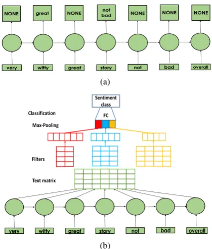
Figure 1:The PBLM model (figures imported from ZR18). (a) The PBLM representation learning model. (b) PBLM-CNN where PBLM represen-tations feed a CNN task classifier.
from ZR18) for adaptation of a sentiment classi-fier between book reviews and reviews of kitchen appliances. In this example PBLM learns the connection between the book related (and hence non-pivot) adjectivewitty, and great- a common positive adjective in both domains, and hence a pivot. PBLM is designed to feed structure-aware task classifiers. Particularly, in the PBLM-CNN architecture that we consider here (Figure 1b),4 the PBLM’s softmax layer (that computes the probabilities of each pivot to be the next uni-gram/bigram) is cut and a matrix whose columns are the PBLM’shtvectors is fed to the CNN.
ZR18 demonstrated the superiority of PBLM-CNN over previous approaches to DReL, estab-lishing the importance of structure-aware repre-sentation learning for review document modeling. We hence develop our TRL methods for PBLM.
3 Task Refinement Learning for PBLM
We apply TRL only to the representation learn-ing stage of the unsupervised domain adapta-tion pipeline. We first describe the general TRL
4ZR18 also considered a PBLM-LSTM architecture
where the PBLM representations feed an LSTM classifier. We focus on PBLM-CNN which demonstrated superior per-formance in 13 of 20 of their experimental setups.
scheme, and then list specific implementations.
3.1 A General TRL Scheme
As noted in § 2, PBLM is similar to an LSTM language model, but instead of predicting the next word at each position, it predicts the next unigram or bigram if these are pivots and a special NONE symbol otherwise. Our TRL scheme gradually ex-poses pivots to PBLM (Algorithm 1).
We start by dividing the pivot features into two subsets: PosPiv is the set of pivot features that are more frequent in source domain training doc-uments with positive labels than in source domain documents with negative labels; NegPiv is simi-larly defined, but these pivots are more frequent in source domain training documents with a negative label. In the first stage, PBLM is trained on the unlabeled data from the source and the target do-mains till convergence, just as in ZR18. The only difference is that in cases where the next unigram or bigram is a pivot, instead of predicting the ac-tual pivot identity, PBLM should predictPosPivor NegPivaccording to the pivot’s class. That is, the representation learned by the first PBLM model is only sensitive to whether a pivot is positive or negative and not to the actual pivot identity. Fol-lowing the definition of pivot features (§ 2), the positive/negative distinction is fundamental, and is hence considered at the first TRL stage.
Data:Us: unlabeled source domain data;Ut: unlabeled target domain data.
Input:K: number of TRL iterations;
SortPivots: a sorted array of pivots;NegPiv: the list of negative pivots;PosPiv: the list of positive pivots.
θ0 = rand();
θ1 = PBLMTrain (θ0, NegPiv, PosPiv,Us,
Ut); i = 1;
whilei≤Kdo
θ= update-PBLM-params (θi, NegPiv, PosPiv, SortPivots, i);
θi+1= PBLMTrain (θ, NegPiv, PosPiv, SortPivots, i,Us,Ut);
i = i + 1;
end
returnθi;
Algorithm 1:TRL for PBLM.
iter-ations (denoted withKin Algorithm 1). The algo-rithm receives as input a sorted array of pivot fea-tures such that pivots at the beginning of the array (lower indices) should be exposed first. At each it-eration the PBLM is exposed to additional#P/K pivots, where#P is the total number of pivot fea-tures. That is, at the first iteration the first#P/K pivots are exposed, at the second iteration the next
#P/K are also exposed and so on till the last (K-th) iteration in which all pivots are exposed. Since new features are exposed in each iteration, the la-bel space of PBLM changes. For example, before the first iteration the label space consists of three labels: NONE, PosPiv and NegPiv, while in the first iteration the label space consists of NONE, PosPiv (for all positive pivots that are not exposed in this iteration), NegPiv (for all negative pivots that are not exposed in this iteration) and the first (top ranked)#P/K pivots in the sorted pivot ar-ray, for a total of#P/K+ 3 labels.
At each iteration the algorithm first updates the PBLM parameters (up-PBLM-params method of Algorithm 1). In this step a new PBLM model is initialized such that all its parameters except for those of the softmax prediction matrix are initial-ized to the parameters to which PBLM converged in the last time it was trained. The softmax matrix grows so that it can predicti·#P/K+ 3labels, instead of (i−1)·#P/K + 3 labels as in the previous PBLM training (i is the iteration num-ber). To do that, the weights for the NONE, PosPiv and NegPiv classes as well as for the pivots that were exposed before the current iteration are ini-tialized to the output of the previous PBLM train-ing, while the weights of the newly exposed piv-ots are initialized to the weights learned for PosPiv (for those newly exposed pivots that were assigned the PosPiv label in the previous run) or for Neg-Piv (for those newly exposed pivots that were as-signed the NegPiv label in the previous run). Af-ter the parameAf-ters are initialized, PBLM is trained again and the process proceeds iteratively till the last iteration where all the pivots are exposed. The weights of the last iteration will be used when PBLM is employed at the classification stage of the unsupervised DA pipeline (§2).
Example To make the above explanation more concrete, we consider an example in which we have four pivots: good, bad, great and worst, so that good and great belong to PosPiv while bad andworst belong to NegPiv. We setK, the
number of iterations, to 2, which means that the number of features exposed in each iteration is
#P/K = 4/2 = 2. Finally, we assume that our
pivot ranking method ranks the pivots in the order in which they were presented above.
PBLM is first trained so that at each position if the next word is good or great it should predict PosPiv, if it isbadorworstit should predict Neg-Piv and otherwise it should predict NONE. Then the pivot exposure iterations begin. At the first it-eration the pivotsgoodandbadare exposed. The parameters learned in the previous run of PBLM (with the PosPiv, NegPiv and NONE predictions) are used as an initialization of the PBLM parame-ters, except that the softmax matrix should now al-low five classes: PosPiv (for occurrences ofgreat, that has not been exposed yet), NegPiv (for occur-rences of worst), good, bad and NONE. Hence, in the softmax matrix of the new PBLM the pa-rameters for PosPiv, and also for good, will be the parameters learned in the previous iteration for PosPiv. Likewise, the parameters for NegPiv, and also for bad, will be the parameters learned in the previous iteration for NegPiv, and the parameters for NONE are those previously learned for NONE. At the second iteration, the last two pivots,great andworst, are also exposed, and PBLM now has the following 5 classes: good, bad, great, worst and NONE. Parameter initialization is done in a similar manner to the first iteration, where the soft-max parameters forgreatandworstare initialized to the parameters of PosPiv and NegPiv of the pre-vious PBLM, respectively. Finally, this last PBLM is trained to yield the model that will be used in the unsupervised DA setup.
We next describe our three methods for the or-der in which pivots are exposed in TRL training.
3.2 Pivot Exposure in TRL
not consider any target domain information. Another alternative is the Ranking by Fre-quency (RF)method that ranks pivots according to the number of times they appear in the unla-beled data of both the source and target domains (combined). The reasoning here is that the repre-sentation learning model should have more statis-tics about the frequent pivots, which makes their prediction easier. Moreover, the frequent piv-ots presumably provide a more prominent signal about the desired representation and should hence be learned prior to less frequent pivots, whose sig-nal is more nuanced. One obvious advantage of this method is that it considers both the source and the target domain. However, in cases where a pivot is very frequent in one domain and substantially less frequent in the other, RF would consider this pivot frequent, even though it does not provide too much information about one of the domains.
To overcome this limitation of RF, we also consider a third pivot ranking method: Rank-ing by Similar Frequencies (RSF). In this method we compute two quantities for each pivot:
fp−source = ##ps
sd andfp−target =
#pt
#td, where#ps
is the number of times the pivotp appears in the source domain unlabeled data, #sd is the num-ber of documents in the source domain labeled data, and #pt and #td are defined similarly for the target domain unlabeled data. We then com-pute the similar frequency score of each pivot p
to be: f reqScore(p) = min(fp−source,fp−target)
max(fp−source,fp−target),
and rank the pivots in a descending order of
f reqScore scores. This way, pivots with more
similar frequencies in the unlabeled data of both domains are ranked higher and will be exposed earlier to the PBLM algorithm.
4 Experiments
We implemented the setup of ZR18, including datasets, baselines, and hyperparameter details.
Task and Domains Following ZR18, and a large body of DA work, we experiment with the task of binary cross-domain sentiment classifica-tion with the product review domains of Blitzer et al. (2007) – Books (B), DVDs (D), Electronic items (E) and Kitchen appliances (K). We also consider the airline review domain that was pre-sented by ZR18, who demonstrated that adapta-tion from the Blitzer product domains to this do-main, and vice versa, is more challenging than adaptation between the Blitzer product domains.
For each of the domains we consider 2000 labeled reviews, 1000 positive and 1000 nega-tive, and unlabeled reviews: 6000 (B), 34741 (D), 13153 (E), 16785 (K) and 39396 (A). Since PBLM is computationally demanding, and em-ploying TRL to PBLM requires multiple PBLM training processes, we pick 6 setups from the 20 of ZR18. We include each of the domains consid-ered in ZR18 at least once. Our setups are: B-D, B-K, E-D, K-B, A-B and K-A.
Models and Baselines Our main baseline is the PBLM-CNN sentiment classifier – the supe-rior model of ZR18 (§ 2) – to which we refer as NoTRL. Our TRL algorithm aims to improve the PBLM (representation learning) step of the PBLM-CNN model. We consider the three TRL methods of § 3.2: Ranking by MI (RMI), Rank-ing by Frequency (RF), and Ranking by Similar Frequencies (RSF), each protocol is implemented with either K = 4 or K = 2 iterations, in ad-dition to the initial step where the pivots are split into the positive and negative classes. The model names are hence: RMI2, RMI4, RF2, RF4, RSF2 and RSF4. To evaluate the relative importance of the initial pivot split to positive, negative and non-pivot classes compared to the non-pivot exposure meth-ods, we also add theBasicTRLmodel in which the basic three class PBLM training is followed by a single iteration where all the pivots are exposed.
To put our results in the context of previous leading models we further compare to the promi-nent baselines of ZR18: AE-SCL-SR; SCL with pivot features selected using the mutual infor-mation criterion(SCL-MI, (Blitzer et al., 2007)); MSDA and MSDA-DAN (Ganin et al., 2016) which employs a domain adversarial network (DAN) with MSDA vectors as input. Finally, we compare to a NoDA setup where the sentiment classifier is trained in the source domain and ap-plied to the target domain without adaptation. For this case we consider a logistic regression classi-fier that was demonstrated in ZR18 to outperform LSTM and CNN classifiers. This is also the clas-sifier employed with AE-SCL-SR and SCL-MI.5
Features and Pivots The input features of all models are word unigrams and bigrams. The di-vision of the feature set into pivots and non-pivots is based onBlitzer et al.(2007) and (Ziser and
Re-5The URLs of the datasets and the code we used, are
ichart,2017,2018a): Pivot features appear at least 10 times in the unlabeled data of both the source and the target domains, and among those features are the ones with the highest mutual information with the task (sentiment) label in the source do-main labeled data. For non-pivot features we con-sider unigrams and bigrams that appear at least 10 times in the unlabeled data of at least one domain.
Cross-Validation and Hyperparameter Tuning
We employ a 5-fold cross-validation protocol as in ZR18. In all five folds 1600 source domain ex-amples are randomly selected for training data and 400 for development, such that both the training and the development sets have the same number of positive and negative reviews. For each model we report the averaged performance across these 5 folds. For previous models, we follow the tuning process of ZR18. The tuning of PBLM and of our TRL methods is described in the Appendix.
5 Results
Overall Performance Our first result is pre-sented in Table1. On average across the test sets, all TRL-PBLM methods improve over the original PBLM (NoTRL) with the best performing method, RF2, improving by as much as 2.1% on average (80.9 vs. 78.8). In all 6 setups one of the TRL-PBLM methods performs best. In two setups RF2 improves over NoTRL by more than 3.5%: 80.2 vs 75 (E-D) and 86.1 vs 82.5 (B-K) (error reduc-tion of 20.8% and 20.6%, respectively). In two other setups RF2 improves by 1.7-2%: K-B (76.2 vs. 74.2), and A-B (72.3 vs. 70.6). In the remain-ing two setups a TRL method improves, although by less than 0.5%. The 80.9% averaged accuracy of RF2 compares favorably also with the 74.4% of AE-SCL-SR, the strongest baseline from ZR18.
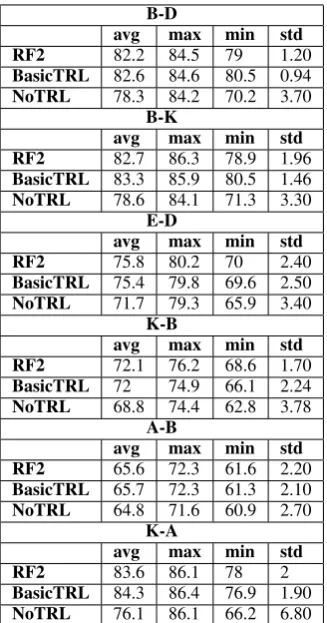
Test Set Stability Our second result is presented in Table 2. The table presents the minimum (min), maximum (max), average (avg) and stan-dard deviation (std) of the test set scores of the 30 hyper-parameter configurations we consider for each model. The table compares these numbers for RF2, our best performing TRL-PBLM method, BasicTRL, that exposes all the pivots in the first iteration after PBLM is trained with the positive, negative and non-pivot classes, and for NoTRL.
The table clearly demonstrates that RF2 and Ba-sicTRL consistently achieve higher avg, max and min results, as well as a lower std, compared to
adaptation with NoTRL. This means that models learned by TRL based methods are much more ro-bust to the selection of the hyper-parameter con-figuration. Moreover, even the min values of RF2 consistently outperform the NoDA model (where a classifier is trained on the source domain and ap-plied to the target domain without domain adapta-tion; bottom line of Table1) and the min values of BasicTRL outperform NoDA in 5 of 6 setups (av-erage difference of 3.9% for RF2 and for 3.5% for BasicTRL). In contrast, the min value of NoTRL is outperformed by NoDA in 5 of 6 cases (with an averaged gap of 2.8%).
Model Selection Stability Additional compari-son between Table 2 and Table 1 further reveals that model selection by development data has a more negative impact on NoTRL, compared to RF2 and BasicTRL. Particularly, for NoTRL there are only two cases where the model that performs best on the test set (max column of Table2) was selected by the development data (the numbers re-ported in Table1): B-D (84.2%) and K-A (86.1%). Moreover, the averaged difference between the best test set model and the one selected by the de-velopment data for NoTRL is 1.3%, and in one setup (E-D) the difference is as high as 4.3%. For RF2, in contrast, there are four cases where the best performing test set model is selected by the development data (E-D, K-B, A-B and K-A), and the averaged gap between the selected model and the best test set model is only 0.1%. For Basic-TRL the corresponding numbers are two setups and an averaged difference of 0.6%. These im-proved stability patterns are observed also with the other TRL methods we experiment with. We do not provide additional numbers in order to keep our presentation concise.
Finally, we note that BasicTRL preforms well, despite being simpler than the other TRL models. For example, in three of the six Table1setups Ba-sicTRL is the second best model and in one setup it is the best model. Table 2also reflects similar performance for RF2 and BasicTRL. Likewise, for all pivot exposure methods 2 iterations are some-what better than 4. In future work we intend to explore additional pivot exposure strategies.
B-D B-K E-D K-B A-B K-A Average
PBLM+TRL Methods
RF2 84.1 86.1 80.2 76.2 72.3 86.1 80.9
RF4 83.4 85 79.2 73.7 71 86.5 79.8
RSF2 84 85.1 79.1 74 71.3 85.9 79.9
RSF4 83.4 85.3 78 74.1 69.7 86 79.4
RMI2 83.5 85.4 79.2 74.1 69.6 86.2 79.7
RMI4 83.5 84.9 78.1 72.8 69.4 86.1 79.1
BasicTRL 84.4 85.9 78.2 74.6 70.8 86.4 80.1
Plain PBLM (ZR18)
NoTRL 84.2 82.5 75 74.2 70.6 86.1 78.8
Other Baselines
AE-SCL-SR 81.1 80.1 74.5 73 60.5 76.9 74.4
MSDA 78.3 78.8 71 70 58.5 76.8 72.2
MSDA-DAN 79.7 75.4 73.1 71.2 59.5 76.6 72.6
SCL 78.8 77.2 70.4 69.3 61.7 72.3 71.6
[image:8.595.142.457.61.304.2]NoDA 76 74 69.1 67.6 57.5 69.6 67
Table 1: Sentiment accuracy when hyper-parameters are tuned with development data.
B-D
avg max min std RF2 82.2 84.5 79 1.20
BasicTRL 82.6 84.6 80.5 0.94
NoTRL 78.3 84.2 70.2 3.70
B-K
avg max min std RF2 82.7 86.3 78.9 1.96
BasicTRL 83.3 85.9 80.5 1.46
NoTRL 78.6 84.1 71.3 3.30
E-D
avg max min std RF2 75.8 80.2 70 2.40
BasicTRL 75.4 79.8 69.6 2.50
NoTRL 71.7 79.3 65.9 3.40
K-B
avg max min std RF2 72.1 76.2 68.6 1.70
BasicTRL 72 74.9 66.1 2.24
NoTRL 68.8 74.4 62.8 3.78
A-B
avg max min std RF2 65.6 72.3 61.6 2.20
BasicTRL 65.7 72.3 61.3 2.10
NoTRL 64.8 71.6 60.9 2.70
K-A
avg max min std
RF2 83.6 86.1 78 2
BasicTRL 84.3 86.4 76.9 1.90
NoTRL 76.1 86.1 66.2 6.80
Table 2: Statistics of the test set accuracy distribution achieved by the PBLM-CNN sentiment classifier, when adapted between domains with RF2, BasicTRL, and NoTRL (the first two are TRL-based methods). The statistics are computed across 30 model configurations.
B-D B-K E-D K-B A-B K-A RF2 98.4 98.9 99.3 98.6 99.5 99.2
B-TRL 97.9 99.0 99.2 95.5 99.0 98.4
NoTRL 78.2 81.7 81.2 78.3 72.5 76.1
Table 3: Ablation analysis. B-TRL is BasicTRL.
This encoding (the hidden vectors of the LSTM) is then fed to the task classifier. We can hence expect that in a high quality PBLM model the representa-tion of pivots (their vectors in the softmax output matrix of the model) from the PosPiv class (§3.1) will be similar to each other, and the representa-tion of pivots from the NegPiv class will be similar to each other, but that members of the two classes will have distinct representations. This way we are promised that the input text encoding preserves an important bit in the pivots’ semantics: their corre-spondence to one of the sentiment labels.
[image:8.595.100.264.360.672.2]NoTRL BasicTRL RF2
pivot sentiment pivot sentiment pivot sentiment
would recommend positive would highly positive would recommend positive love positive would recommend positive would highly positive recommend them positive happy positive recommend them positive
remember positive recommend positive happy positive
not recommend negative recommend them positive love positive
happy positive enjoyed positive I highly positive
thought negative only complaint positive remember positive would not negative appreciate positive recommend positive
not buy negative I highly positive never have positive
I highly positive saves positive appreciate positive
Table 4: Top 10 nearest neighbors (ranked from the closest neighbor downward) of the pivot ”highly recom-mended” according to three models: NoTRL (plain PBLM), BasicTRL and RF2. TRL training results in all members of the neighbor list of a pivot being of the same sentiment class as the pivot itself.
NegPiv clusters compared to the pivot representa-tions in NoTRL. This means that the encoding of the input with respect to the pivots preserves the sentiment class information much better in these TRL models than in the NoTRL model.
To illustrate this effect, we present here a qual-itative example of the nearest neighbor list of a pivot according to three models (Table4). The do-main adaptation setup of the example is K-A and the pivot we selected for this example is highly recommended which falls into the PosPiv class (i.e. it appears many more times in positive source domain reviews than in negative ones). The table demonstrates that for the NoTRL model there are several NegPiv pivots in the nearest neighbor list ofhighly recommended– e.g.not recommendand not buy. In contrast, the nearest neighbors lists of highly recommended according to BasicTRL and RF2 contain only pivots from the PosPiv class.
6 Conclusions
We proposed Task Refinement Learning algo-rithms for domain adaptation with representation learning. Our TRL algorithms are tailored to the PBLM representation learning model of ZR18 and aim to provide more effective training for this model. The resulting PBLM-CNN model improves both the accuracy and the stability of the original PBLM-CNN model where PBLM is trained without TRL.
In future work we would like to develop more sophisticated TRL algorithms, for both in-domain and domain adaptation NLP setups. Moreover, we would like to establish the theoretical groundings
to the improved stability achieved by TRL, and to explore this effect beyond domain adaptation.
Acknowledgements
We would like to thank the members of the IE@Technion NLP group for their valuable feed-back and advice. This research has been funded by an ISF personal grant on ”Domain Adaptation in NLP: Combining Deep Learning with Domain and Task Knowledge”.
References
Shai Ben-David, John Blitzer, Koby Crammer, Alex Kulesza, Fernando Pereira, and Jennifer Wortman Vaughan. 2010. A theory of learning from different domains.Machine learning, 79(1-2):151–175.
Yoshua Bengio, J´erˆome Louradour, Ronan Collobert, and Jason Weston. 2009. Curriculum learning. In Proceedings of the 26th annual international con-ference on machine learning, pages 41–48. ACM.
John Blitzer, Mark Dredze, Fernando Pereira, et al. 2007. Biographies, bollywood, boom-boxes and blenders: Domain adaptation for sentiment classi-fication. InProc. of ACL.
John Blitzer, Ryan McDonald, and Fernando Pereira. 2006.Domain adaptation with structural correspon-dence learning. InProc. of EMNLP.
Danushka Bollegala, Takanori Maehara, and Ken-ichi Kawarabayashi. 2015. Unsupervised cross-domain word representation learning. InProc. of ACL.
Ciprian Chelba and Alex Acero. 2004. Adaptation of maximum entropy capitalizer: Little data can help a lot. InProc. of EMNLP.
Minmin Chen, Yixin Chen, and Kilian Q Weinberger. 2011. Automatic feature decomposition for single view co-training. InProc. of ICML.
Minmin Chen, Zhixiang Xu, Kilian Weinberger, and Fei Sha. 2012. Marginalized denoising autoen-coders for domain adaptation. InProc. of ICML.
St´ephane Clinchant, Gabriela Csurka, and Boris Chidlovskii. 2016. A domain adaptation regulariza-tion for denoising autoencoders. In Proc. of ACL (short papers).
Hal Daum´e III. 2007. Frustratingly easy domain adap-tation. InProc. of ACL.
Hal Daum´e III and Daniel Marcu. 2006. Domain adap-tation for statistical classifiers. Journal of Artificial Intelligence Research, 26:101–126.
Jeffrey L Elman. 1993. Learning and development in neural networks: The importance of starting small. Cognition, 48(1):71–99.
Yaroslav Ganin, Evgeniya Ustinova, Hana Ajakan, Pascal Germain, Hugo Larochelle, Franc¸ois Lavi-olette, Mario Marchand, and Victor Lempitsky. 2016. Domain-adversarial training of neural net-works. Journal of Machine Learning Research, 17(59):1–35.
Xavier Glorot, Antoine Bordes, and Yoshua Bengio. 2011. Domain adaptation for large-scale sentiment classification: A deep learning approach. InIn proc. of ICML, pages 513–520.
Chen Gong, Dacheng Tao, Stephen J Maybank, Wei Liu, Guoliang Kang, and Jie Yang. 2016. Multi-modal curriculum learning for semi-supervised im-age classification.IEEE Transactions on Image Pro-cessing, 25(7):3249–3260.
Stephan Gouws, GJ Van Rooyen, MIH Medialab, and Yoshua Bengio. 2012. Learning structural corre-spondences across different linguistic domains with synchronous neural language models. In Proc. of the xLite Workshop on Cross-Lingual Technologies, NIPS.
Sepp Hochreiter and J¨urgen Schmidhuber. 1997. Long short-term memory. Neural computation, 9(8):1735–1780.
Jiayuan Huang, Arthur Gretton, Karsten M Borgwardt, Bernhard Sch¨olkopf, and Alex J Smola. 2007. Cor-recting sample selection bias by unlabeled data. In Proc. of NIPS.
Frank Hutter, Holger Hoos, and Kevin Leyton-Brown. 2014. An efficient approach for assessing hyperpa-rameter importance. InProc. of ICML.
Jing Jiang and ChengXiang Zhai. 2007. Instance weighting for domain adaptation in nlp. In Proc. of ACL.
Diederik Kingma and Jimmy Ba. 2015. Adam: A method for stochastic optimization. In Proc. of ICLR.
Diederik P Kingma and Max Welling. 2014. Auto-encoding variational bayes. InProc. of ICLR.
Christos Louizos, Kevin Swersky, Yujia Li, Max Welling, and Richard Zemel. 2016. The variational fair autoencoder.
Yishay Mansour, Mehryar Mohri, and Afshin Ros-tamizadeh. 2009. Domain adaptation with multiple sources. InProc. of NIPS.
David McClosky, Eugene Charniak, and Mark John-son. 2010. Automatic domain adaptation for pars-ing. InProc. of NAACL.
Quang Nguyen. 2015. The airline review dataset.
https://github.com/quankiquanki/
skytrax-reviews-dataset. Scraped from
www.airlinequality.com.
Junhyuk Oh, Xiaoxiao Guo, Honglak Lee, Richard L Lewis, and Satinder Singh. 2015. Action-conditional video prediction using deep networks in atari games. InProc. of NIPS.
Sinno Jialin Pan, Xiaochuan Ni, Jian-Tao Sun, Qiang Yang, and Zheng Chen. 2010. Cross-domain senti-ment classification via spectral feature alignsenti-ment. In Proceedings of the 19th international conference on World wide web, pages 751–760. ACM.
Anastasia Pentina, Viktoriia Sharmanska, and Christoph H Lampert. 2015. Curriculum learning of multiple tasks. InProc. of CVPR, pages 5492–5500.
Nils Reimers and Iryna Gurevych. 2017. Reporting score distributions makes a difference: Performance study of lstm-networks for sequence tagging. In Proc. of EMNLP.
Danilo Jimenez Rezende, Shakir Mohamed, and Daan Wierstra. 2014. Stochastic backpropagation and ap-proximate inference in deep generative models. In Proc. of ICML.
Brian Roark and Michiel Bacchiani. 2003. Supervised and unsupervised pcfg adaptation to novel domains. InProc. of HLT-NAACL.
Alexander M Rush, Roi Reichart, Michael Collins, and Amir Globerson. 2012. Improved parsing and pos tagging using inter-sentence consistency constraints. InProc. of EMNLP-CoNLL.
Tobias Schnabel and Hinrich Sch¨utze. 2014. Flors: Fast and simple domain adaptation for part-of-speech tagging. Transactions of the Association for Computational Linguistics, 2:15–26.
Yangyang Shi, Martha Larson, and Catholijn M Jonker. 2015. Recurrent neural network language model adaptation with curriculum learning. Computer Speech & Language, 33(1):136–154.
Valentin I Spitkovsky, Hiyan Alshawi, and Daniel Ju-rafsky. 2010. From baby steps to leapfrog: How less is more in unsupervised dependency parsing. In Proc. of NAACL-HLT.
Ivan Titov. 2011. Domain adaptation by constraining inter-domain variability of latent feature representa-tion. InProc. of ACL.
Joseph Turian, Lev Ratinov, and Yoshua Bengio. 2010. Word representations: a simple and general method for semi-supervised learning. InProc. of ACL.
Pascal Vincent, Hugo Larochelle, Yoshua Bengio, and Pierre-Antoine Manzagol. 2008. Extracting and composing robust features with denoising autoen-coders. InProc. of ICML.
John Wieting, Mohit Bansal, Kevin Gimpel, and Karen Livescu. 2016. Charagram: Embedding words and sentences via character n-grams. In Proc. of EMNLP.
Yi Yang and Jacob Eisenstein. 2014. Fast easy unsu-pervised domain adaptation with marginalized struc-tured dropout. InProc. of ACL (short papers).
Jianfei Yu and Jing Jiang. 2016. Learning sentence em-beddings with auxiliary tasks for cross-domain sen-timent classification. InProc. of EMNLP.
Yang Zhang, Philip David, and Boqing Gong. 2017. Curriculum domain adaptation for semantic seg-mentation of urban scenes. In The IEEE Interna-tional Conference on Computer Vision (ICCV), vol-ume 2, page 6.
Yftah Ziser and Roi Reichart. 2017. Neural structural correspondence learning for domain adaptation. In Proc. of CoNLL.
Yftah Ziser and Roi Reichart. 2018a. Pivot based lan-guage modeling for improved neural domain adap-tation. In Proceedings of the 2018 Conference of the North American Chapter of the Association for Computational Linguistics: Human Language Tech-nologies, Volume 1 (Long Papers), volume 1, pages 1241–1251.
Yftah Ziser and Roi Reichart. 2018b. Deep pivot-based modeling for cross-language cross-domain transfer with minimal guidance. InProceedings of the 2018 Conference on Empirical Methods in Natural Lan-guage Processing, pages 238–249.
A URLs of Code and Data
As noted in the experiments section, we provide here the URLs for the code and data we use in the paper.
• Blitzer et al. (2007) product review data: http://www.cs.jhu.edu/
˜mdredze/datasets/sentiment/
index2.html.
• The airline review data is (Nguyen,2015).
• Code for the PBLM and PBLM-CNN models (Ziser and Reichart, 2018a):
https://github.com/yftah89/
PBLM-Domain-Adaptation.
• Code for the AE-SCL and AE-SCL-SR models of ZR17 (Ziser and Reichart, 2017):
https://github.com/yftah89/
Neural-SCLDomain-Adaptation.
• Code for the SCL-MI method ofBlitzer et al.
(2007): see footnote6 (the URL does not fit into the line width).
• Code for MSDA (Chen et al.,2012):http:
//www.cse.wustl.edu/˜mchen.
• Code for the domain adversarial network used as part of the MSDA-DAN baseline (Ganin et al., 2016): https://github. com/GRAAL-Research/domain_
adversarial_neural_network.
• Logistic regression code: http:
//scikit-learn.org/stable/.
B Hyperparameter Tuning
As noted in the experimental setup, for all previ-ous work models (except from the PBLM mod-els of (Ziser and Reichart,2018a)), we follow the experimental setup of (Ziser and Reichart,2017) including their hyperparameter estimation proto-col. The hyperparameters of the PBLM models are provided here (they are identical to those of (Ziser and Reichart,2018a)):
• Input word embedding size:(128,256).
• Number of pivot features:
(100,200,300,400,500).
6https://github.com/yftah89/
structural-correspondence-learning-SCL
• |ht|: (128,256,512).
• PBLM model order: second order.
Note that Ziser and Reichart(2018a) also con-sidered the word embedding size of 32 and 64. In our preliminary experiments these hyper-parameters provided very poor performance for the plain PBLM model, so we excluded them from our full set of experiments.
For the CNN in PBLM-CNN we only experi-mented withK = 250filters and with a kernel of sized= 3.
All the algorithms in the paper that involve a LSTM or a CNN are trained with the ADAM algo-rithm (Kingma and Ba,2015). For this algorithm we used the parameters described in the original ADAM article (these parameters were also used by ZR18):
• Learning rate:lr= 0.001.
• Exponential decay rate for the 1st moment es-timates:β1= 0.9.
• Exponential decay rate for the 2nd moment estimates:β2 = 0.999.
• Fuzz factor:= 1e−08.
• Learning rate decay over each update:
decay= 0.0.
For all the experiments in the paper we use the same random seed for parameter initialization.
C Experimental Details
Pre-processing All sequential models consid-ered in our experiments are fed with one review example at a time. For all models in the paper, punctuation is first removed from the text before it is processed by the model (sentence boundaries are still encoded). This is the only pre-processing step we employ in the paper. This decision is in line withZiser and Reichart(2018a).