Munich Personal RePEc Archive
The Center and the Periphery: Two
Hundred Years of International
Borrowing Cycles
Kaminsky, Graciela
George Washington University
22 October 2017
Online at
https://mpra.ub.uni-muenchen.de/82125/
The Center and the Periphery:
Two Hundred Years of International Borrowing Cycles
Graciela Laura Kaminsky Department of Economics
George Washington University and NBER Washington, DC 20052
Email: graciela@gwu.edu http://home.gwu.edu/~graciela
October 2017
Abstract
A common belief in both academic and policy circles is that capital flows to the emerging periphery are excessive and ending in crises. One of the most frequently mentioned culprits is the cycles of monetary easing and tightening in the financial center. Also, many focus on the role of crises in the financial center, pointing to excess international borrowing predating crises in the financial center and global retrenchment in capital flows in its aftermath. I re-examine these views using a newly-constructed database on capital flows spanning two hundred years. Extending the study of capital flows to the first episode of financial globalization has two major advantages: During this episode, monetary policy in the financial center is constrained by the adherence to the Gold Standard, thus providing a benchmark for capital flow cycles in the absence of an active role of central banks
in the financial centers. Second, panics in the financial center are rare disasters that
need to be examined in a longer historical episode. I find that boom-bust capital flow cycles in the periphery are milder in the second episode of financial globalization when the financial center follows a cyclical monetary policy. Also, cyclical monetary policy in the financial center is far more pronounced in times of crises in the financial center, cutting short capital flow bonanzas in the periphery and injecting liquidity in the aftermath of the crisis.
Keywords: International borrowing cycles, systemic and idiosyncratic capital flow bonanzas.
JEL Codes: F30, F34, F65
1
I.Introduction
The booms and busts in international capital flows since the restart of capital mobility in the 1970s have attracted a lot of attention in both academic and policy circles. Many suggest that capital flow bonanzas are excessive, ending in crises, and leading to protracted declines in
international issuance.1 While the culprits behind the boom-bust cycles are many, the most
frequently mentioned are the cycles of monetary easing and tightening in the financial centers. It is further argued that these monetary cycles trigger highly synchronized international capital flows
unrelated to countries’ specific macroeconomic conditions, the so-called global financial cycle.2
The empirical research on the role of monetary policy in the financial center on international capital flow cycles focuses on the easing in the mid-1970s, the one in the early 1990s, and most recently the one in the early 2000s. With just a few cycles, it is hard to pinpoint the role of monetary policy in the financial centers on the rest of the world. This is especially so because these cycles coincide with other worldwide shocks, such as the oil shocks of the 1970s, the creation of the European Monetary Union in the 1990s, or the savings glut in East Asia in the early 2000s. Another aspect of booms and busts in capital flows that has attracted attention more recently is the role of crises in the financial center. Many have pointed to the global retrenchment in capital flows in the aftermath of the 2008 Subprime Crisis in the United States (see, for example, Boussière, Schmidt, and Valla, 2016). This slowdown in international borrowing has been accompanied by a protracted collapse in the global economy quite different from the one following previous capital flow bonanzas and busts. While the boom-bust borrowing cycle in Latin America, Asia, Russia, and Turkey in the 1990s also ended with crises, those crises were short-lived with the periphery rapidly rebounding. Importantly, those crises erupted amid highly liquid international capital markets with a healthy financial center and a growing world economy, with vulnerabilities only present in the crisis countries. In contrast, the 2008 crisis had the financial center at its epicenter, with international capital markets collapsing and the world economy coming to a standstill. It is hard to draw general conclusions about crises with the financial center at its epicenter from just examining the crisis of 2008.
1 See, for example the IMF World Economic Outlook (2016); Broner, Didier, Erce, and Schmukler (2013); Forbes
and Warnock (2012); Ghosh, Qureshi, Kim, and Zalduendo (2014); Reinhart and Reinhart (2009).
2
In this paper, I study international capital flow cycles during a far larger episode. I look at the first episode of financial globalization that starts with the end of the Napoleonic Wars in the
early 19th century and ends with the Great Depression in 1931 when barriers to international capital
flows and trade are erected around the globe as well as the second episode of financial globalization that starts with the collapse of the Bretton Woods System in the 1970s. Studying the dynamics of capital flows during these two episodes has two advantages. First, during the first episode of financial globalization, monetary policy in the financial center is constrained by the adherence to the Gold Standard, providing a benchmark for capital flow cycles in the absence of an active role
of central banks in the financial centers. Second, panics in the financial center are rare disasters.3
Thus, to understand the empirical regularities of this type of global crises, we need to look at a longer historical episode. The first episode of financial globalization spanning more than 100 years is witness to major crises in the financial center, such as the London panic in 1825, the world crisis in 1873 fueled by the collapse of financial markets in continental Europe, the 1890 Baring Crisis in London, and the crisis following the collapse of financial markets in New York and London in 1929.
I constructed a new database of international capital flows spanning two hundred years. The data for the first episode of financial globalization was collected in London, Paris, Frankfurt
and Berlin, and New York, the financial centers of the 19th and early 20th centuries, using
information in archives, prospectuses, annual reports of the stock markets, and financial newspapers of those times. The database collected includes public international issuance (central governments, provinces/states, and municipalities) as well as international issuance by private financial and non-financial corporations. The database is granular. It includes data on every bond and share floated in international capital markets. For bonds, it includes the amount issued, the interest rate, the issue price, the amortization characteristics, the underwriting banks, as well as information on the markets those bonds were floated. For shares, the database includes the amount issued, the price of issue, as well as whether shares are ordinary or preferred. A similar database is constructed for the episode 1970-2015. The database for the 1970s is collected from the Archives of the World Bank while the data starting in 1980s is from various digital databases as well as data from the IMF, the Institute of International Finance, and Central Banks. The database constructed for the period 1970-2015 is also granular and includes all the bonds, syndicated loans, and shares
3
floated in international capital markets. The database on international issuance is complemented with a database on economic fundamentals, including economic activity, commodity prices, terms of trade, world interest rates, inflation, and monetary statistics, all going back to 1820.
The focus of attention in this study is on Latin American countries. These countries started to participate in international capital markets right after independence from Spain and Portugal in
the first twenty years of the 19th century. I study the characteristics of booms and crashes in
international gross primary issuance for each Latin American country, with a focus on duration and amplitude. For each cycle, I calculate the increase in indebtedness using the information on gross issuance and the amortization characteristics of bonds and loans as well as the effects of defaults and restructurings. Cycles in private and public gross issuance are then studied separately
to examine their contribution to the boom-bust cycle in international gross primary issuance.4 The
characteristics of these cycles are then compared across these two episodes of financial globalization. Finally, I study the effects of idiosyncratic and global economic and financial conditions on booms and busts in international borrowing by the emerging periphery.
The main results of the paper indicate that:
First, although many have argued that cyclical monetary policy in the financial center since
the 1970s is at the core of volatile and excessive booms and busts in capital flows to the emerging periphery, capital flow bonanzas and crashes are far more pronounced during the first episode of financial globalization when monetary policy in the financial center is constrained by the adherence to the Gold Standard.
Second, the differences in the magnitude of the booms and busts of capital flows to the
emerging periphery in the first and second episode of financial globalization are mainly driven by capital flow cycles around crises in the financial center. During the first episode of financial globalization, capital flows during the bonanzas that precede panics in the financial center are about 60 percent larger than those bonanzas during tranquil times while capital flows during the busts that follow the crisis in the financial center are just half of those during tranquil times. In contrast, international capital flows to the emerging periphery around crises in the financial center since the 1970s are characterized by smaller bonanzas and substantial more issuance during the bust.
4 This is an important contribution of this paper since while there is partial historical data on central government
4
Third, the changes in monetary regimes in the financial center (from adherence to the Gold
Standard to autonomous monetary policy since the collapse of the Bretton Woods System) contribute to the time-varying characteristics of international capital flow cycles to the emerging periphery around episodes of crisis in the financial center. Monetary cycles in the financial center are more pronounced when the financial center is at the epicenter of the crisis, with protracted contractions cutting short the bonanza episodes and persistent expansions injecting more liquidity in international capital markets during the busts.
The rest of the paper is organized as follows. Section II provides a short chronology of global capital flow cycles and Latin American countries’ participation in international capital markets. Section III describes the new database as well as its sources. This section also describes the construction of the data on international issuance and debt for the seven largest Latin American countries. Section IV examines the characteristics of booms and busts in international gross primary issuance for each Latin American country. This section also compares the borrowing cycles in both episodes, with especial attention to the magnitude of capital flow bonanzas and busts. Section V examines the evolution of the domestic economy as well as world-wide shocks around the peak of the capital flow cycles to Latin America. Section VI concludes.
II. Global Capital Flows and Latin America’s International Borrowing, 1820-20155
The first international capital flow bonanza starts in the early 1820s. At the core of this cycle is the increase in liquidity fueled by the sharp decline in military spending following the end of the Napoleonic wars, with London as the new financial capital of the world. This capital flow bonanza engulfs Europe, with Denmark, Russia, Spain, and a variety of independent Italian States (Naples, Piedmont, Tuscany, and the Papal States) floating bonds in London. This bonanza also spreads to Latin America. All Latin American countries (except Puerto Rico and Cuba) gain independence from Spain and Portugal in the early 1800s. The new independent countries immediately eliminate the restrictions to trade imposed on the colonies by Spain and Portugal. International trade starts and participation in international capital markets soon follows. The first Latin American country to float bonds in London is Gran Colombia. The first issue is in 1820 for
5 The chronology of capital flows and crises during the 19th and early 20th centuries is partly based on Bordo and
5
547,784 British pounds. By the end of 1825, Latin American’s total international issuance has reached 20 million British pounds.
The boom ends in the summer of 1825 when the Bank of England raises the discount rate to stop the drain of reserves fueled by the import boom and the outflow of capital. The tightening of liquidity is followed by a stock market crash in October, a banking panic in December, and numerous bankruptcies. The financial debacle in London rapidly spreads to continental Europe, with bankruptcies of major banks in Germany, Italy, Amsterdam, Saint Petersburg, and Vienna. The crisis extends rapidly to Latin America as overseas loans are cut off. This is not all. The crisis also triggers a major fiscal problem in Latin America. As world trade collapses, so do tariff revenues, the only source of income of the governments of the new countries with Argentina, Brazil, Chile, the Federation of Central America, Colombia, Mexico, and Peru defaulting starting in 1826.
International issuance restarts in the 1830s. This time around the United States is the most important borrower. It is not the federal government but the U.S. states the ones at the heart of the capital flow bonanza. By the end of the 1830s, nineteen U.S. states and two territories have issued bonds, with debt increasing by a factor of thirteen in just ten years. Most of the debt is issued abroad, primarily in London (see English, 1996). The bonanza also reaches European countries while Latin American countries, still in default, are not able to tap international capital markets in this period. The boom ends in 1839 following the tightening of credit by the Bank of England, with the crash in international liquidity partly leading to the default of nine of the U.S. States starting in 1841.
As with previous bonanzas, the collapse in international liquidity is quite prolonged, with international capital flows starting to recover only in the 1850s. The capital flow bonanza now reaches not just Europe but also the Commonwealth countries (Australia, Canada, India, New Zealand, and South Africa). Importantly, the world economy recovery starting in the late 1840s fuels a new boom in demand for primary products and raw materials, benefiting Latin American
economies, in particular, Chile and Peru.6 The growing international trade accompanying the
recovery in Europe fuels a new fiscal bonanza in all Latin American countries (as tariff revenues
6 The export of agricultural and mineral products surges dramatically: Guano from Peru, copper from Chile, wool
6
increase accordingly) and with it the possibility of settlement of the foreign debts.7 Peru is the
first to issue a new bond in London in 1853. Still, the new loan boom to Latin America only
flourishes in the 1860s after the end of the panic of 1857.8
The capital flow bonanza to Latin America starting in the 1860s is larger than that of the early 1820s, with capital flows financing not just governments and the extraction of mineral resources but also the creation of banks and the adoption of cutting edge technologies such as, telegraphs and the construction of railroads. The capital inflows to Argentina, Brazil, Chile, Colombia, Mexico, Peru, and Uruguay during the 1860s and early 1870s reach 132 million British
pounds. The world international capital flow bonanza slows down with the British crisis in 18669
and even more with the crisis of 1873. The end of the Franco-Prussian War in 1870 plays a critical part in the unfolding of the crisis of 1873. Following the defeat of Napoleon III, the new French government pays a huge indemnity of 5,000 million francs (200 million British pounds) to Germany. These indemnity transfers lead to a massive flow of capital into the economics of central Europe, fueling speculation in various financial markets. A spectacular stock market crash in Vienna in May 1873 ends with the stock market boom in Austria and spreads rapidly to Germany. Between 1873 and 1878, half the Austrian banks close, and 400 of the 800 Austrian join-stock companies go bankrupt. Stock markets in Amsterdam and Zurich also crash. The crisis crosses the Atlantic in September, the New York Stock market collapses and is followed with a U.S. banking panic. As during the crisis of 1825, there is a collapse in world trade and in the prices of commodities and loans are called off. Tax revenues in Latin America sharply drop and trigger a new wave of defaults across the region. The steep decline in commodity and stock prices as well as the bank and industrial bankruptcies in most countries start the first worldwide 1873 recession. The crisis is also felt in the Middle East. By 1876 the Ottoman Empire, Egypt, Greece, and Tunisia have defaulted. In total, by the year 1876 fifteen non-European nations have suspended
7 Chile is the first to renegotiate its debt in 1842, Peru follows in 1849. Most Latin American countries renegotiate
their debts in the 1850s.
8 The crisis of 1857 begins in the U.S. A railroad stock boom fueled by British capital and the California gold
discoveries in 1849 crashes in August 1857 with a banking panic. The crisis spreads to England in the Fall. From England, the crisis spread to the continent, with a serious panic in Hamburg in December.
9 The crisis of 1866 is preceded by a large credit expansion both in England and France that triggers a boom in prices
7
payments on almost 30 million British pounds. In Latin America, Bolivia, Colombia, Costa Rica, Guatemala, Honduras, Peru, and Uruguay default on their foreign debt.
While the world depression of the 1873 wreaks havoc around the world, by the early 1880s a process of recovery has begun. The upswing in world economic activity fuels foreign trade and new capital flows to countries in the periphery. Again, as in the 1860s and 1870s, capital flows finance not just governments but also private activities in new industries, such as railways, tramways, construction of ports, gas works, and of course, they also finance the production of raw materials, mining, and land companies. Latin America also benefits from this new capital flow bonanza. From 1874 until late 1880s, international gross primary issuance by the seven largest Latin American countries reaches 280 million British pounds, with Argentina and Uruguay being the most important recipients. The boom of the 1880s ends in 1890 with the crisis set off by the near-failure of Baring Brothers, the underwriter of Argentine Government loans. The Bank of England prevents a panic via a recapitalization of Baring Brothers with the help of other major London financial institutions and loans from the Banque de France and Russia. Still, the crisis spreads back to Latin America with the cessation of British lending to Argentina and Uruguay. Between 1890 and 1894 Argentina, Ecuador, Guatemala, Nicaragua, Paraguay, Uruguay, and Venezuela default. A sharp worldwide decline in the flow of British capital follows this crisis, partly triggering major banking crises in the United States and Australia in 1893.
The next international capital flow cycle starts in the late-1890s and ends with the start of
WWI.10 While Britain continues to be the main creditor, France, German and American investors
set up new companies in banking as well as in railways, tramways, mines, ports, sugar refineries, flour mills, gas works, water works, and even some early electric and telephone companies. This episode is considered until now the heyday of financial globalization. Latin American borrowing in international capital markets during this cycle reaches one billion British pounds. The outbreak of World War I contributes to the end of this boom in international capital flows. In July, as war becomes imminent, a liquidity crunch spreads around the world as investors start to liquidate
10 This boom is interrupted in 1907 with a crisis originating in the United States following the San Francisco
8
foreign assets, fueling panics in all asset markets. While the panic is promptly stopped by the central banks in the United Kingdom, the United States, and continental Europe, the outbreak of the war in Europe causes an abrupt suspension of capital flows. Only Brazil, Ecuador, Mexico, and Uruguay default. This time around, the governments of most nations of the region continue to service their debt using export surpluses.
Capital flows resume with the end of the war in Europe. Increases in productivity due to major inventions, including electricity, automobiles, communications, and petrochemicals as well as, innovations in industrial organization lead to a boom in economic activity that spills over around the world. Most Latin American nations benefit from the continuing rise in international prices of raw materials and primary products. New York becomes the leading financial center while lending from London and Paris retrenches following the imposition of capital controls in
Great Britain and France11 and capital markets in Germany collapse. In 1927-1928 the Federal
Reserve, concerned over stock market speculation, tightens monetary policy; a recession begins in July 1929. Prices of commodities collapse, stock markets around the globe crash, and capital flows sharply decline, precipitating currency and banking crises in Latin America, Europe, and Australia. In September 1931, Great Britain abandons the Gold Standard and so does the United States in 1934. Bolivia, Brazil, Chile, Colombia, Costa Rica, Cuba, Dominican Republic, Guatemala, Nicaragua, Panama, Paraguay, Peru, and Uruguay default. Barriers to capital flows are erected around the globe ending this first episode of financial globalization.
During the next forty years, international capital flows languish amid restrictions to capital mobility in both developed and developing countries only to recover following the collapse of the Bretton Woods System. Ironically, the revival of international capital markets can be traced to new financial restrictions in Great Britain and the United States in the late 1950s and 1960s. In 1957, the British government introduces new financial restrictions in the vain attempt to stop the speculation against the British pound. In the end, the devaluation is not averted. But the restrictions make London-based banks create a new market to avoid losing their share of financial transactions: Banks’ dollar deposits start to be used to provide dollar loans in an unregulated market, which becomes to be known as the Eurodollar market. In 1964, it is the U.S. turn. This
11 Foreign lending is formally restricted in Great Britain starting in December 1914. While formal restrictions are
9
time, the currency under attack is the U.S. dollar. To stop the speculation, the U.S. government
introduces capital account controls in 1964.12 U.S. based-banks, like their British counterpart in
the 1950s, turn to the Eurodollar market to avoid the restrictions that could imperil their operations, with liquidity in this market sharply increasing.
But perhaps, the straw that broke the camel’s back is the collapse of the Bretton Woods system in 1973. With no need to defend the peg, countries can choose their own monetary policy without the need to restrict capital mobility and thus a new era of financial liberalization begins. As early as July 1973, United States eliminates capital account restrictions. Germany and Great Britain follow, partially eliminating capital controls in 1973 while Japan joins in 1979. In the late 1970s, Latin American countries deregulate the domestic banking sector and eliminate restrictions on international capital flows.
The first international market to develop in the 1970s is the syndicated loan market, particularly with lending to emerging markets. The dramatic surge in international loans is triggered by the oil shock in 1973-74, with the high savings of OPEC countries being channeled through the Eurodollar market particularly during the 1979-81 period. The boom in syndicated lending to emerging markets peaks at 57 billion dollars in 1981. But in 1982 international issuance collapses. At the heart of this collapse are the monetary contraction, recession, and the banking distress in the United States. Mexico’s default in August 1982 adds to the fragility of the commercial banking sector in the United States. With U.S. banks recalling their loans from all emerging markets, other defaults follow. Most of Latin American countries suspend interest and principal payments and they are also followed by countries in Asia, Eastern Europe, and Africa. The rest of the 1980s witness a pronounced downturn in lending to emerging economies: Gross issuance of syndicated loans remains at half of the issuance reached in the early 1980s. With all large U.S. commercial banks heavily exposed to the now emerging countries in default, the policy in the U.S. is to maintain current interest servicing by debtor countries to the U.S. banks, mostly by creating a new plan of “involuntary” loans from the exposed U.S. commercial banks while at the same time promoting continuous negotiations and extending the maturity of the loans. This arrangement allows the banks to keep all their loans on the books at face value, even though they
12 In September 1964, the United States Congress enacts the Interest Equalization Tax (IET), an excise tax on
10
are heavily discounted in the secondary market.13 Monetary policy in the U.S. is also heavily
relaxed to ameliorate the overall distress in the financial sector and reverse the downturn in the economy.
The Brady plan and its initiative to restructure defaulted loans starting in 1989 end with
the isolation of developing markets from international capital markets.14 This time around, both
the government and the private sector start issuing bonds in international capital markets. Latin America benefits especially from the new international bond market. In fact, issuance in the bond market surpasses that of the syndicated loan market, with Latin American countries bond issuance increasing from 2 billion dollars in 1990 to 84 billion dollars in 1997.
The Brady plan also provides a new impetus to the syndicated loan market. Helped by the easy monetary conditions in industrial countries in the early 1990s, syndicated loans reach a new peak at 190 billion dollars in 1997, almost four times higher than the level reached in the early 1980s. This time around, the largest beneficiaries in emerging markets are the East Asian countries, with gross issuance reaching almost 100 billion dollars in 1997. The nationality of lenders also changes: While in the early 1980s most of the syndicates are composed of U.S. banks, in the 1990s Japanese and European banks play a leading role in lending to emerging markets, especially to East Asian countries. The boom in the 1990s in the syndicated loan market is not confined to emerging markets. By 2004 international syndicated lending has increased to 2.5 trillion dollars, with developed countries capturing the lion share of the international syndicated loan market, with gross issuance reaching 1.8 trillion dollars in 2004. Moreover, the expansion of the bond and syndicated loan markets in the 1990s is now accompanied by the development of an international equity market. But the 1990s as the 1980s are plagued by crises. In the aftermath of these crises, net capital flows to Latin America sharply decline with total issuance falling to about 60 percent of its peak in 1997.
The last wave of international lending starts in the early 2000s. While capital flows to all emerging markets, the lion share continues to flow to advanced economies. Total international issuance peaks in 2007. Amid this boom, monetary policy is severely tightened, with the Federal Funds interest rate increasing from 1 percent in 2003 to 5 percent in 2007. As with the bank crisis
13 See Sachs (1986) and Sachs and Huizinga (1987).
14 The key innovation of the Brady Plan is to allow the commercial banks to exchange their claims on developing
11
in the United States in the 1980s, the U.S. monetary policy is dramatically reversed following the panic in the financial centers. The Federal Funds rate sharply declines to zero, and the money base surges, reaching about 25 percent of GDP. Latin America international issuance is only transitorily affected by the 2008 Subprime crisis in the United States. Latin America total international issuance increases until 2014 and peaking at 217 billion dollars, only to decline by 37 percent in 2015.
III. International Issuance: The Database
The historical data for this paper forms part of a database I am constructing of international issuance of both the government and the private sector of all countries that participate in international capitals markets, including countries like Paraguay that floats a few bonds during the first episode of financial globalization to Australia that issues thousands of bonds and shares in international capital markets during the same period. The historical data for this project has been
collected over several years from financial newspapers of the 19th and early 20th centuries, annual
reports of the Stock Markets in London and Paris, the Annual Listings of Bonds and Stocks in the Berlin, Frankfurt, and Hamburg Stock Markets, the archives of the London Stock market, the Paris Bourse, and the New York Stock Exchange, as well as the archives of merchant banks such as the House of Rothschild in London and deposit banks, such as the Credit Lyonnais in Paris. I have also used publications from government agencies in the United States, such as the Department of Commerce and the Federal Reserve. Part of the material has also been collected from important studies on sovereign debt by scholars in Latin America, Asia, and Europe. This database is unique, it includes all issuance in all the financial centers from 1820 to 1931.
12
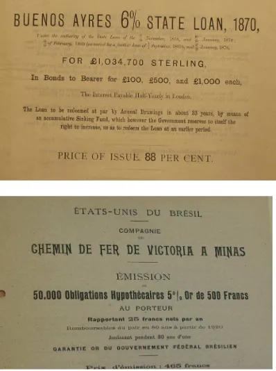
To introduce the historical data, I present two prospectuses in Figure 1.15 The first one is
a 1,034,700 British-pound bond issued by the Province of Buenos Aires (Argentina) in 1870. This is a 6% loan issued at a discount (88 percent of face value) redeemable in 33 years, with interest paid twice a year in London. This bond, as most sovereign bonds in the early phase of financial integration, is callable, allowing governments to refinance their debt in low-interest rate years. The second one is a 5% mortgage bond issued by the Railway Company Victoria to Minas in Brazil in 1911 for 25 million French francs redeemable in 89 years and issued in Paris.
Although not shown in the photos that just include the top part of the prospectuses, these
bonds are, like most of the bonds issued in the 19th and early 20th centuries, sinking fund bonds
similar to current mortgage loans. For example, the Buenos Aires 6% bond has an accumulative sinking fund of 1%. The total annual service of this loan is 7% (1% for the sinking fund and 6% for the coupon rate) of the total amount issued. For the 1,034,700 British pound bond, the annual service is equal to 72,429 British pounds. As with mortgages, the service mostly pays the coupons in the first years of the life of the bond, with the part dedicated to the amortization increasing over time. In the case of the Buenos Aires 6% bond, the service is partly used to amortize the bond by annual drawings of the bond at par. More infrequently, bonds are bullet bonds, with the face value of the principal paid at maturity. The information on repayment characteristics of the bonds is used to estimate net primary issuance (gross primary issuance minus amortization) and to construct series of both public and private debt.
The information in the prospectuses, annual reports of the Stock Markets, or listings in financial newspapers when the bonds are issued only provides the originally planned repayment characteristics of the bond. But most bonds are callable, allowing the borrower to repay earlier the bonds. During the first episode of financial globalization, there are waves of refinancing in low-interest rate years, with old high-coupon bonds converted into newly issued low-coupon bonds. To estimate net issuance and debt series, it is necessary to identify these conversions. The original repayments of the bonds also change when the country defaults. To estimate net issuance and debt it is necessary to study in detail the characteristics of the restructurings. The restructurings of the debt following defaults for Latin America are described in Kaminsky and Vega-García (2016). That paper only studies the defaults and the restructurings of the central
13
government bonds. This paper extends that research to bonds issued by Provinces, States, and Municipalities. It also studies the conversions of bonds issued by private firms.
The data on gross primary issuance that I construct captures access to international capital
markets, that is, it only includes issuance for cash.16 As estimated, gross primary issuance does
not include the value of the bonds issued in exchange for previously issued bonds via a conversion or an exchange of defaulted bonds for new bonds when the default ends. Nor does it include bonds issued to pay accumulated coupon arrears when the debt is restructured to end a default. Finally, net primary issuance is estimated by subtracting cash amortizations from gross primary issuance. In contrast, the debt series include the remaining value of all the bonds issued for cash as well as that of the new bonds issued in conversions or bonds issued in the aftermath of defaults to exchange the original bonds or to pay the accumulated arrears in coupons while eliminating the bonds converted. That is, debt increases with new borrowing and the issuance of bonds to pay coupon arrears as well as with the issuance of conversion bonds and declines with both the amortization of bonds with cash payments or with the newly converted bonds.
I construct a similar database for the second episode of financial globalization starting in 1970. As with the database for the first episode of financial globalization, the database for this period includes the bonds and shares floated in international capital markets. It also includes international syndicated loans. I follow the BIS in the identification of international syndicated loans (See, Gadanecz, 2004) and identify international loans as those loans in which the nationality
of at least one of the syndicate banks differs from that of the borrower.17 The data are collected
from the World Bank Archives as well as from Dealogic and Bloomberg. Since most the countries in the sample defaulted, I collect data on the exchanges following the defaults from Bloomberg, the database of the International Finance Institute, the International Monetary Fund publications, and a variety of studies examining restructurings of debt, such as Sturzenegger and Zettelmeyer (2006).
16 All issuance is measured at face value.
17 The database for both episodes does not include bonds/loans with maturity at issuance less than one year. It does
14
IV. International Borrowing Cycles: Then and Now
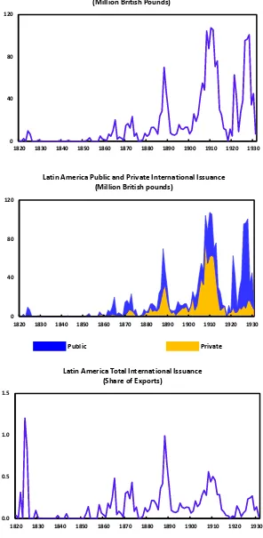
Figure 2 first shows the newly collected data covering the period from 1820 to 1931. This figure shows the international gross primary issuance of Latin America as captured by the issuance of Argentina, Brazil, Chile, Colombia, Mexico, Peru, and Uruguay. These seven countries are the most active participants in international capital markets in the region during the first episode of financial globalization. The top panel shows total gross primary issuance in British pounds, the middle panel decomposes total issuance into public and private issuance. Finally, the bottom panel shows the gross primary issuance/exports ratio to have a measure of participation in international capital markets relative to the size of the economy. As shown in Figure 2, there are clear
boom-bust episodes throughout the 19th and early 20th centuries peaking around 1824, 1865, 1873, 1888,
1910, and 1928.
The boom of the 1820s is mostly due to loans to the governments of the newly independent countries. International issuance of Latin American countries totals 20 million British pounds (at face value). This episode also witnesses the creation of new companies in the mining sector. In total, twenty-eight companies are formed with a proposed capitalization of 24 million British pounds. However, by the time of the collapse in the summer of 1825, the shares issued amounted only to 3.5 million British pounds.
15
through issues of bonds, mortgage bonds, and equity issuance. Some of the earlier issues are those of the Brazilian Street Railway in 1869, the Sao Paulo Railway in 1870, City of Buenos Aires Street Railway in 1870, and Buenos Aires National Tramways Limited also in 1870. While the expansion is slowed down by the Overend Gurney crisis in London in 1866, by the early 1870s Latin American countries are heavily participating in international capital markets again. In this episode, Peru becomes the most indebted country in Latin America, with its foreign debt increasing to 36 million British pounds in 1876 from 7 million British pounds in 1856. The collateral provided by the exports of guano, monopolized by the Peruvian government, allows Peru’s government to access international capital markets in such grand way.
After the crisis in 1873, the next lending cycle peaks in 1888. From 1874 until the onset of the Baring crisis in 1890, the accumulated gross primary issuance of these seven countries reaches 280 million British pounds. The next cycle of capital issuance peaks around 1910. From 1890 until the start of the first war capital flows to Argentina, Brazil, Chile, Colombia, Mexico, Peru, and Uruguay almost reach 1 billion British pounds. A large part of international issuance finances the construction of railways and tramways, ports, gas works, and water drainages. Other areas financed by international capital flows are land development, coffee and sugar plantations, production of nitrates, and general mining operations. The last capital flow bonanza starts in 1918 and peaks in 1928. From 1918 to 1931, the accumulated total gross issuance by the seven countries totals about 600 million British pounds
16
Information on total issuance is insufficient to compare the extent of financial integration during this episode. We need to scale total issuance with an indicator of the size of the economy. The most common indicator used to capture the extent of integration across countries is the ratio
of total issuance (or capital flows) to GDP. Official estimates of GDP for the 19th century and
even the early 20th century are not available. Instead, I use exports as the scale variable.18 Figure
2 bottom panel shows the issuance/exports ratio. Average issuance/exports is 15 percent during the first episode of financial globalization starting in 1820 and ending in 1931 with a peak at 121 percent in 1824.
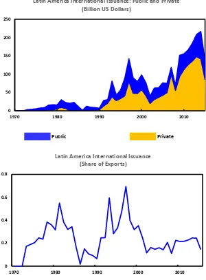
Figure 2 also shows similar graphs for the second episode of financial globalization, 1970-2015. The top panel shows Latin America international gross issuance in US dollars. This panel shows clearly three cycles with peaks in 1981, 1997, and 2014. The second panel shows the decomposition of issuance into public and private. As in the first episode of financial globalization, the first cycle is mostly about government borrowing. In contrast, the bonanzas of the 1990s and the 2000s are on average 60 percent private issuance. The bottom panel shows total issuance as a share of exports. Interestingly, the capital flow bonanza of the 2000s is milder than those of the earlier periods when issuance is scaled by exports.
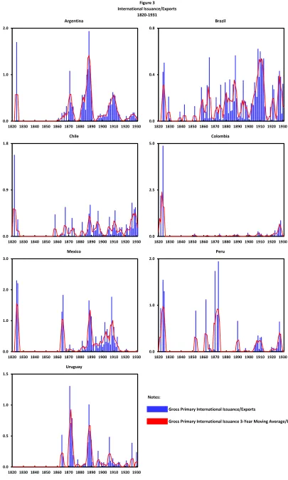
I now examine in more detail the capital flow cycles for the seven countries in the sample. Figure 3 shows gross international primary issuance for each country as a share of exports. The blue bars in this figure show international issuance (as a share of exports). Data on issuance is quite volatile, in large part because government bonds are issued in big tranches. To have a better visualization of booms and busts, the red line in Figure 3 also shows international primary issuance as a three-year moving average (as a share of exports). As shown in Figure 3, during the first episode of financial globalization, booms and busts in international issuance across the seven
countries are highly correlated, with mostly all countries participating in each cycle.19 There are
two exceptions. Following the boom of the 1820s, all Latin American countries default. These defaults last around 30 years. Following the debt restructurings mostly in the 1850s, Argentina, Brazil, Chile, Peru, and Uruguay start tapping international capital markets again in the 1860s. In
18 Exports are quite volatile. For the issuance/export ratio to capture the volatility of capital flows only, I use trend
exports as the scale variable. Trend exports are estimated using the Hodrick-Prescott filter.
19 Uruguay is a province of Brazil during the capital flow bonanza of the 1820s, gaining independence in 1828. It taps
17
contrast, Colombia and Mexico, amid serial defaults,20 are out of international capital markets until
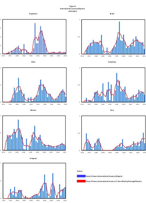
the beginning of the 20th century and the 1880s respectively.21 The figures for the second episode
of financial globalization also show that cycles are highly correlated across the countries. With the exception of Argentina following the default of 2001, all countries participate in the capital flow bonanzas of the 1970s, 1990s, and 2000s.
I will now examine more systematically the boom-bust capital flow cycles, their duration and amplitude. To identify the boom-bust cycles in gross international issuance, I apply the
algorithm used to identify business cycles.22 The first step in the determination of the cycles is the
identification of the cyclical turning points. The algorithm that I am going to apply looks for clearly defined swings in total issuance with at least a minimum duration similar to that of business cycles and a minimum issuance (as a share of exports) at the peak of the cycle of 15 percent. Essentially, the algorithm isolates local minima and maxima in a time series, subject to the constraint on the length of upturns and downturns and the constraint of a minimum issuance at the peak of the cycle.
I impose the restriction that the cycle cannot have duration of less than 5 years. That is, 𝑦𝑦𝑡𝑡
(international issuance as a share of exports) is a maximum if:
𝑦𝑦𝑡𝑡−2,𝑦𝑦𝑡𝑡−1< 𝑦𝑦𝑡𝑡 < 𝑦𝑦𝑡𝑡+1,𝑦𝑦𝑡𝑡+2 (1)
and 𝑦𝑦𝑡𝑡 is at least 0.15.23 The trough is identified as the minimum value between two local peaks.
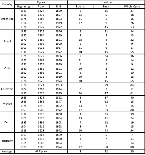
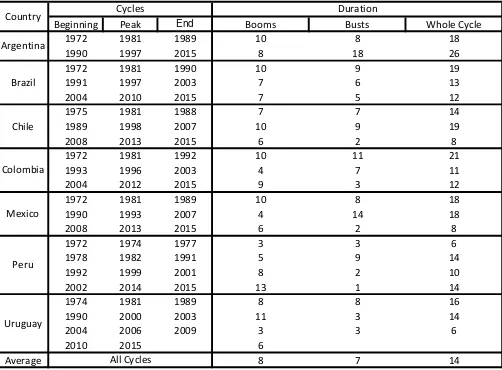
I apply this filter to the (3-year moving average) total issuance/exports ratio for each of the seven countries in the sample. The algorithm identifies 34 cycles for the first episode of financial globalization and 22 for the second episode of financial globalization. Table 1 shows the characteristics of these cycles. The average duration of the capital flow bonanzas is 8 years across the two episodes. For the first episode of financial globalization, the minimum boom duration is of 2 years and the maximum boom duration is of 18 years. For the second episode of financial globalization, the minimum boom duration is 3 years and the maximum boom duration is of 13 years. Interestingly, the length of the bust during the first episode of financial globalization is
20 During the period 1826 to 1905 Colombia defaults 5 times, with Colombia being in default in total for 70 years.
Mexico defaults twice, in 1827 and in 1854. The first default last 25 years and the second lasts 33 years.
21 Even in default, Mexico taps international capital markets in the 1860s during the French intervention from 1861 to
1867. During the intervention, the French government imposes Maximiliam I as emperor. During this period, the government of Maximiliam I issues bonds in Paris. After the French intervention is defeated, Benito Juárez is re-elected president and the loans contracted by the government of Maximiliam I are repudiated.
22 See, for example, Bry and Boschan (1971), Harding and Pagan (2002), and Kaminsky and Schmukler (2008).
23 I impose a minimum issuance of 15 percent of exports at the peak of the cycle to identify bona fide bonanza cycles
18
more varied. The minimum duration of the bust is 2 years. Capital flow crashes can last much longer. For example, Colombia after the capital flow bonanza of the 1820s and amid serial defaults cannot tap international capital market for 79 years. But long-lasting bust spells may be due to global patterns. For example, following the Great Depression in 1931, barriers to capital flows are erected around the world with international capital markets disappearing for about 40 years. Latin American countries start tapping international capital markets only in the 1970s. The duration of the crashes during the second episode of financial globalization is less volatile than that of the earlier episode, with the most protracted bust lasting 18 years (for Argentina following
the default of 2001) and the shortest lasting 2 years.24
To examine the magnitude of the capital flow bonanzas and capital flow busts, I need to
estimate the accumulated net issuance during the boom and during a bust.25 I estimate the
amplitude of the bonanza (bust) for each cycle i as follows:
i i
i
i
T T
t
t
i
X
issuance net
amplitude
∑
=
= 1 (2)
Where 1 is the year when the capital flow bonanza (bust) starts. For bonanzas, T is the year of the
peak of the capital flow cycle and the numerator is total accumulated net issuance over the boom
normalized by the level of exports in the year of the peak of the cycle. For busts, T is the year of
the trough of the capital flow cycle and the numerator is total accumulated net issuance over the bust normalized by the level of exports in the year of the trough of the cycle.
I now examine whether capital flow bonanzas and busts can be classified into different varieties.
IV.1 Varieties of Capital Flow Cycles
This section studies and tests whether the characteristics of bonanzas and busts change from the first episode to the second episode of financial globalization. It also examines whether capital flow cycles in the emerging periphery change depending on whether there is a crisis in the financial center. As I discussed in the previous section, the first episode of financial globalization
24 Note that the last cycle for all countries is incomplete, so I cannot compute the complete duration of some of the
cycles of the 2000s.
25 Issuance includes both issuance of bonds and shares for the first episode of financial globalization and includes
19
was mired in panics with the financial center at its epicenter. As examined in a variety of chronologies (see, for example, Bordo and Murshid (1999) and Kaminsky and Vega-García,
(2016)), the most virulent crises in the 19th and early 20th centuries are the 1825 crisis in London,
the 1873 crisis in continental Europe, the Baring crisis in London in 1890, and the London and New York 1929 crisis that heralded the Great Depression. The second episode of financial globalization is witness to two worldwide financial crises with the financial center at its epicenter. The first crisis erupts in the United States in the early 1980s. The crisis bursts amid the tightening in monetary policy in the United States and is preceded by a large boom in international lending
to emerging markets by large U.S. commercial banks.26 This crisis spreads around the globe,
triggering crises in Latin America, Eastern Europe, and Africa. The second crisis in the financial center erupts in 2008, the so-called U.S. Subprime financial crisis. The crisis spreads to advanced economies around the world and almost triggers the collapse of the European Monetary Union. The crisis lingers for a decade with a collapse in economic activity around the world. I classify
the capital flow cycles around a crisis in the financial center as Systemic Capital Flow Cycles,27
with all the cycles unrelated to panics in the financial center being identified as Idiosyncratic
Capital Flow Cycles.
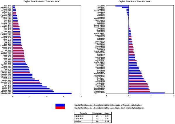
I first examine the characteristics of cycles then and now. Table 2 shows the amplitude of booms and busts (estimated as shown in (2)) in international borrowing. For the first episode of financial globalization, 1820-1931, the average capital flow bonanza is quite pronounced, with total accumulated net issuance across all countries averaging 194 percent of exports. Still, the amplitude of the cycles is quite varied with some bonanzas being extremely large and reaching almost seven hundred percent of exports and others much milder with accumulated total net issuance being just a fraction of exports during the cycle. Interestingly, some of the most extreme capital flow bonanzas occur in the 1820s, with Colombia and Mexico’s bonanzas reaching seven and four hundred percent of their exports at the peak of the cycle. Not surprisingly, Colombia’s
26 The boom in international lending to emerging economies is not just a U.S. banking sector affair. Japanese banks
and U.K. banks and some other European banks also participate in the lending boom, although the large U.S. commercial banks are the ones most heavily exposed to emerging markets in this first boom in international lending since the 1920s. See Sachs and Huizinga (1987).
27 A capital flow cycle is identified as systemic if capital flow bonanza starts before the onset of the crisis in the
20
and Mexico’s default spells following this boom are the longest, with endless restructurings until their debt burdens reach sustainable levels.
During the bust in capital flows, net issuance declines substantially to about 25 percent of exports. Importantly, 30 percent of those busts are more extreme. During these extreme crashes, countries are unable to tap international capital markets, with zero or even negative accumulated net issuance during the downturn in the cycle. The sharpest decline in issuance occurs in Peru following the 1873 world crisis. At that time, Peru’s accumulated net issuance becomes negative, with the deleveraging reaching 58 percent of exports.
The estimates in Table 2 for the episode of 1970-2015 paint a different picture of capital flow booms and busts. The average capital flow bonanza for this episode is 113 percent of exports and only 60 percent of the average capital flow bonanzas in the earlier episode. In contrast, the average accumulated net issuance during the busts in the modern episode is larger than the one in the earlier period of globalization, with accumulated issuance during the bust averaging 38 percent of exports. Interestingly, extreme crashes are less prevalent since the 1970s, only accounting for 5 percent of all the cycles, suggesting better access of Latin American countries to international capital markets in bad times.
Figure 4 tests whether capital flow bonanzas and busts in the earlier period are systematically different than those in the current period. As shown in this figure, the null hypothesis of equal bonanzas in the first and second episodes of financial globalization can be rejected with a p-value of 0.01. Bonanzas in the first episode of financial globalization are 72 percent larger than those during the second episode of financial globalization. The accumulated net issuance during the busts during the second episode of financial globalization is about 50 percent larger than that during the first episode of financial globalization. The null hypothesis of equality of busts across the two episodes can be rejected at a p-value equal to 0.09.
21
cycles following the crisis in 2008, busts following crises in the financial center are not different from those observed during tranquil times. The p-value is equal to 0.25.
Figure 6 examines whether the characteristics of systemic and idiosyncratic cycles change over time. The first episode of financial globalization is witness to four major crises in the financial center: 1825, 1873, 1890, and 1929. These crises are preceded by more extreme capital flow bonanzas. The average bonanza in Latin America for cycles preceding panics in the financial centers reaches 226 percent of exports, with the average bonanza unrelated to these global panics only reaching 142 percent of exports. As shown in Figure 6, the null hypothesis of equality of
systemic and idiosyncratic bonanzas can be rejected with a 0.05 p-value. The estimates shown for
the episode of 1970-2015 paint a complete different picture of capital flow bonanzas. The average capital flow bonanza to Latin America preceding the financial crises in the United States in the early 1980s and in 2008 only reaches 111 percent of exports and not far from the bonanzas in tranquil times, which average 115 percent of exports. In fact, the null hypothesis of equality of systemic and idiosyncratic bonanzas during the second episode of financial globalization cannot be rejected at any conventional significance level (p-value equal to 0.44).
Figure 6 also examines the characteristics of issuance during bad times. Interestingly, during the first episode of financial globalization, countries have less access to international capital markets in the aftermath of a panic in the financial center when compared to idiosyncratic crashes. Following panics in the financial center, Latin American countries cannot access international capital market, with issuance during the bust only reaching 19 percent of exports. In contrast, issuance during idiosyncratic busts reaches 35 percent of exports. The Null Hypothesis of equality can be rejected at a 0.10 confidence level. Interestingly, during the second episode of financial globalization Latin America countries issuance in the aftermath of crisis in the financial center reaches 59 percent of exports more than three times the issuance during idiosyncratic cycles that only reaches 15 percent of exports. Again, the hypothesis of equality of issuance during busts in these two varieties of cycles can be rejected at all conventional levels (p-value equal to 0.00).
22
4 and 6 for the two episodes of financial globalization suggests that we need to re-evaluate the role of monetary policy in the financial centers.
The previous results focus exclusively on similarities and differences in access to capital markets over phases of booms and busts. They leave unanswered questions about continuous access to international capital markets, the characteristics of the crashes, and overall volatility in access to international capital markets in the first and second episodes of financial globalization. To test whether international capital markets behave differently in these two episodes, I estimate separately the frequency distributions of annual capital flows in the 1820-1931 and 1970-2015 episodes for each country and compare these two distributions using the Kolmogorov-Smirnov
test of equality of distributions.28 Figure 7 shows these results. This figure first reports the
histograms of annual international issuance/exports for the first and second episode of financial globalization for each country. Note that in the first episode of financial globalization the histograms show fat tails, indicating many years of no access to international capital markets as well as many years in which countries can tap heavily international capital markets. The histograms for the second episode of financial globalization suggest a more uniform distribution with similar probabilities of no access, mild access, and high access to international capital markets over the 45 years of the second episode of financial globalization. The results from the Kolmogorov-Smirnov test are reported to the right of the histograms in Figure 7. Note that in all cases, we can reject the null hypothesis of equality of the distributions at conventional significance values.
V. What Fuels Capital Flow Cycles?
The previous section has shown that capital flow cycles have changed over time. Systemic capital flow bonanzas in Latin America have become much less dramatic and undistinguishable from the idiosyncratic ones. Busts have also changed, with Latin American countries being able to tap international capital markets more often during bad times. Still, the ability to tap international capital markets following panics in the financial center and in times of no crisis in the financial center has changed. During the first episode of financial globalization, issuance in
28 The Kolmogorov–Smirnov test is a nonparametric test of the equality of probability distributions. It can be used to
23
the aftermath of panics in the financial center is about half the issuance during busts in tranquil times. In contrast, during the second episode of financial globalization, the ability to tap international capital markets in the aftermath of a crisis in the financial center is far larger than that in the aftermath of idiosyncratic bonanzas. What is driving these differences? Is it country-specific economic conditions? Or are global factors? This section examines the drivers of these differences.
V.1 Global and Idiosyncratic Fundamentals
To capture country-specific shocks, the “pull-factor,” I use two indicators: exports and the terms of trade of the Latin American countries. Since Latin American countries start tapping
international capital markets in the early 19th century and the data on GDP start later in the 20th
century, I capture economic activity using exports. Even data on exports are not readily available for the earlier part of the sample. In many cases, the database on exports is constructed using the data on imports from the most important trade-partner countries. For the terms of trade, I collect data on the prices of the most important exports of each of the countries in the sample and construct an export price index with weights capturing the time-varying share of each commodity export in total exports. I use the wholesale price index of the United Kingdom to capture prices of imports for the first episode of financial globalization and the consumer price index of the United States for the second episode of financial globalization. Figure 8 shows the evolution of country exports and the terms of trade. The first section shows the historical data while the second section shows the data since 1970.
24
first for the episode 1820-1931 and second for the episode 1970-2015.29 The vertical lines in
Figure 9 identify the major panics in the financial centers in our sample.
For the first episode, the top panel shows the U.K. bank rate. This panel clearly shows that panics in the financial center are in part triggered by increases in interest rates. These hikes in interest rates are short-lived. The bottom panel shows the evolution of world imports. Panics in the financial center are followed by persistent declines in world imports. It takes 10 and 14 years respectively for world imports to recover to the pre-crisis level following the panics of 1825 and 1931. Not as long lasting, but still protracted, are the shocks to world imports following the crises of 1873 and 1890. It takes 7 and 8 years respectively for world imports to reach pre-panic levels after these crises. Importantly, part of the collapse of world imports reflects the long-lasting deflation following these crises, with import prices falling for at least 10 years.
For the second episode, the top panel in Figure 9 shows the U.S. Federal Funds interest rate. Again, crises in the financial center are preceded by hikes in the Federal Funds rate. As for the first episode of financial globalization, these hikes in interest rates are reversed at the onset of crises in the financial center. The bottom panel shows the evolution of world imports. As in the first episode of financial globalization, the evidence since 1970 indicates that the world economy slows down more abruptly in the aftermath of panics in the financial center.
To shed light on whether capital flow cycles may have different roots in the first and second episode of financial globalization or whether fundamentals behave differently in episodes with panics in the financial center (systemic episodes), I examine the evolution of these fundamentals around the peaks in international capital cycles of the seven Latin American countries in the
sample. Figure 10 examines capital flows in Latin America as well as the evolution of
country-specific factors (the “pull factors”) as captured by the growth rates of (real) exports and the terms
of trade during idiosyncratic and systemic episodes.30 Each panel in Figure 10 portrays a different
variable. In each panel, the horizontal axis records the number of years before and after the peak of the capital flow cycle. I look at the behavior of each indicator for an interval of 10 years around
29 The database on macro fundamentals for the first episode of financial globalization was initially constructed for
Kaminsky and Vega-García (2016). The database on macro fundamentals for the second episode of financial globalization was constructed using data from WDI, the IMF database, and the Board of Governors of the Federal Reserve System database.
30 For the first episode of financial globalization, I estimate real exports by deflating exports in British pounds with
25
the year of the peaks in capital flows in each country (t). In each figure, the solid line represents
the average behavior of each indicator across all cycles while the dotted lines denote plus/minus one-standard-error bands around the average. To examine whether Latin America countries’ international issuance and fundamentals behave differently around a crisis in the financial center in comparison to those episodes with no crisis in the financial center, Figure 10 shows two columns: the panels to the left show the behavior of all the indicators around the peak of idiosyncratic episodes (episodes with no crisis in the financial center) and the right panels show the same evidence for systemic episodes (episodes with crises in the financial center). For all the variables, the vertical axis in each figure records the percentage-point difference between the value of each indicator during the 10-year interval around the peak relative to its sample mean.
26
Figure 10 also shows the behavior of issuance, exports, and the terms of trade during the second episode of financial globalization. During this episode, the issuance cycles around crises in the financial center are very similar to those of an idiosyncratic nature with peaks reaching about 30 percent of exports and far smaller than the peaks of systemic cycles during the first episode of financial globalization. Interestingly, while capital flows in systemic episodes are not as volatile as those in the first episode of financial globalization, economic fundamentals booms and busts continue to be quite volatile with protracted downturns in the aftermath of panics in the financial center. For example, as shown in the next panel, the growth rate of exports declines from about 5 percentage points above the average to 7 percentage points below the average growth during this episode. Similarly, terms of trade growth declines about 8 percentage points from the peak of the boom to the trough of the bust. In contrast, export and terms of trade growth rates, after a short decline, recover during the bust in capital flows during idiosyncratic capital flow cycles.
Figure 11 shows the evolution of global factors (“push factors”) around the time of the peak in capital flow bonanzas in Latin America. This figure first shows two indicators of global liquidity. The first measure examines the evolution of the interest rate in the financial center
around the peak of the capital flow cycles in Latin America.31 The second measure captures the
aggressiveness and persistence of changes in monetary policy by estimating the 3-year average percent change in interest rates over the capital flow cycle. The last panels show the state of the
world economy as captured by the growth rate of real imports of the financial centers.32 The
indicators in the top and the bottom panels in this figure are shown relative to their average over the sample. The first section of Figure 11 reports the evidence from the historical episode and the second one shows the modern episode.
For the historical episode, the evidence from the top four panels indicate that interest rate changes in the U.K. are not at the core of booms and busts in international capital flows in Latin America. Interest rates and interest rate changes (although they are somewhat volatile) are similar to the averages over the sample. Naturally, during the Gold Standard period, the Bank of England has less room to conduct monetary policy or to become the lender of last resort. The last panels
31 Since any meaningful measures of expectations of inflation for the first episode of financial globalization are
difficult to come by, I use nominal interest rates to capture changes in monetary policy during both episodes of financial globalization. The results are mostly unchanged when I use the real interest rate for the second episode of financial globalization.
27
capture economic activity in the financial centers. Again, as in Latin America, the fluctuations in economic activity in the financial centers are far more pronounced when the center itself is in crisis, with growth rates declining by 4 percentage points between booms and busts in these episodes. In contrast, idiosyncratic cycles in Latin America are accompanied by continuous growth in the world economy.
The second episode of financial globalization presents a different picture about monetary policy in the financial center during systemic and idiosyncratic capital flow cycles. As shown in the top two panels, interest rate fluctuations in the United States in episodes with no crisis in the center are quite small and not statistically different from their average during the sample. In contrast, interest rate policy is more volatile at the onset of the U.S. banking crisis in the 1980s and the Subprime crisis in the 2000s. The Federal Reserve raises interest rates from about 1 percent in 2003 to 5 percent in 2007. Even more strongly, the tightening in monetary policy in the late 1970s and early 1980s fuels an increase in the Federal Funds rate from 5 percent in 1976 to 16 percent in 1981. Importantly, following the onset of the crisis in the financial center, interest rates are sharply reduced, with interest rates declining from 16 percent in 1981 to 7 percent in 1986 during the U.S. banking crisis in the 1980s and from 5 percent in 2007 to a range 0-0.25 percent five years later in the aftermath of the U.S. Subprime crisis. These sharp increases in interest in the years preceding financial crises in the United States cut short the booms in international issuance, with the easy monetary policy in the following years ameliorating the collapse in international capital flows. Interestingly, global economic activity volatility continues to be as pronounced around panics in the financial center as it is during the first episode of financial globalization.
28
both for crisis times and for the entire episode. For both episodes of financial globalization, panics are preceded by interest rate hikes and followed by interest rate reductions. Interestingly during the first episode of financial globalization, hikes and reductions of interest rates around the onset of a crisis in the financial center are not very different from 5-year events over the entire episode. This is not the case during the second episode of financial globalization. On average, 5-year hikes and reductions in interest rate during crises are about 85 percent higher than their averages during the entire episode.
VI. Conclusions
Boom-bust cycles in international capital flows are hardy perennials. Financial globalization erupts in the aftermath of the Napoleonic wars with London at its center. The next 120 years are witnessed to a massive expansion of financial flows to every corner of the globe not just from London but also from Paris, Frankfurt, Berlin, and New York, the new financial capitals of the world. Financial globalization collapses in the aftermath of the Great Depression when countries around the world erect barriers to international capital flows. It takes about 40 years for capital flows to restart. The collapse of the Bretton Woods System heralds the restart of financial globalization. With floating exchange rates, countries can regain monetary autonomy without resorting to capital account controls. Barriers to capital flows begin to be dismantled first in the financial centers and then in the periphery. Financial globalization erupts again and so do boom-bust cycles in international capital flows.
Naturally, the literature on capital flows has grown dramatically. One of the most studied
topics are the triggers of booms and busts, with a focus on the pull and push factors and whether