factors of

J. Range Manage.

56: 425-431 September 2003

Economics of sale weight, herd size, supplementation, and seasonal factors

RUSSELL TRONSTAD AND TRENT TEEGERSTROM

Authors are Associate Professor and Extension Specialist, and Research Specialist, Department of Agricultural and Resource Economics, College of Agriculture and Life Sciences, The University of Arizona, Tucson, Ariz. 85721-0023.

Abstract

A growth function for range calves is estimated using a polyno- mial function of calf age that accounts for weather variation, sex,

prior calf weights relative to a norm, and a compensatory gain factor. Data on rainfall plus calf weights at birth and when calves were roughly 3, 8, 12, and 20 months of age are used to estimate the growth function. This function is then used to determine the economic trade-off between herd size and calf sale weights, for both spring and fall sale dates. In addition, the profitability of feeding supplement is evaluated by increasing the rate of gain beyond that projected by the the polynomial age growth function for southeast and central Arizona grazing environments when forage and nutrients are limited. Using prices from 1980 to 1998, results indicate that the most profitable herd mix, sale date, and feeding protocol for the southeast Arizona region is 204 kg calves with no supplemental feeding and ^sales occurring in May.

Supplemental feeding and sales occurring at 250 kg head1 in May is the most profitable herd mix for the central Arizona region.

More favorable average daily gain rates for May sales from the central versus southeast is why supplemental feeding is marginal- ly better for the central region than feeding no supplement.

Key Words: optimal calf sale weight, livestock supplementation effects, livestock marketing, polynomial age growth function, rainfall

Resumen

Se estimo una funcion de crecimiento para becerros en pastiza- les uuando una funcion polynomial de la edad del becerro que toma en cuenta la variacion de clima, el sexo, los pesos de becer- ro relativos a la norma _y un factor de ganancia compensatoria.

Datos de precipitacion, del peso de los becerros al nacimiento _y del peso cuando tenian aproximadamente ^3, 8,12 _{y 20} meses se usaron para estimar la funcion de crecimiento. Luego esta fun- cion se use para determinar los sacriticios economicos entre el tamano del hato _{y los} pesos de yenta de los becerros, tanto para fechas de yenta de primavera como de verano. Adicionalmente, se evaluo la rentabilidad de suplementar para incrementar la tasa de ganancia mas alla de to proyectado por la funcion polino- mial de edad de crecimiento para ambientes de apacentamiento del sudeste _y la region central de Arizona cuando el forraje _{y los} nutrientes son limitantes. Usando precios de 1980 a 1998, los resultados indican que la mezcla de hato, fecha de yenta _y proto- col de alimentacion mas rentables para la region sudeste de Arizona es becerros de 204 kg sin suplementacion _y las ventas realizadas en Mayo. La alimentacion suplementaria _y las ventas en Mayo con pesos de 250 kg cabeza

¹

es la mezcla de hato mas rentable para la region central de Arizona. Las tasas promedio de ganancia diaria de peso mas favorables en Mayo de la region central versus la region sudeste es la razon por la que la ali- mentacion suplementaria es marginalmente mejor para la region central que el no suplementar.

The trade-off between sale weight and timing of sales is com- plicated by seasonal forage and price conditions along with varia- tion in the price spread between light and heavy calves.

Generally, lighter calves sell for a higher price per unit of weight than heavier calves and calf prices in the spring are greater than in the fall, but exceptions to these generalities occur. In addition, variability in seasonal rainfall and the ability to feed supplement complicates analyzing trade-offs between rates of gain, sale weight, herd size, and the timing of calf sales.

Some ranches have adopted a rather rigid selling practice for their calves to take advantage of seasonal forage availability and aggregate numbers for a given sale to attract more buyers. For example, ranchers in the central region of Arizona typically sell calves in the spring while southeast Arizona ranchers generally sell in the fall. Both regions sell mainly according to the time of year, irrespective of the weight of their calves, and very few feed substantial supplements. Because Arizona ranchers often question the economic trade-offs between calf sale weights, herd size, rates of gain and feeding supplement, and a spring versus fall sale

Manuscript accepted 14 Oct. 02.

date, the primary objective of this analysis was to address these issues. More specifically, the profitability of an Animal Unit (AU) grazing resource is quantified with and without supplemen- tal feeding under the different sale weights of either 159, 204, 250, 295, or 340 kg head' for May and November sale dates from 2 different Arizona regions. In addition, the economic impact of a fertility increase in conjunction with supplemental feeding and the profitability of heavier calf weights during "extra grass" years are evaluated.

Quantifying the future rate of gain for a calf kept on the ranch is a critical element for evaluating the profitability of different marketing dates. Selling calves at a heavier weight generally comes with an opportunity cost of reducing the number of cows that can be maintained on the ranch, thus also reducing the num- ber of calves that can be sold. Several studies have looked at ani- mal performance under different range conditions ^with a produc- tion focus and little economic analysis (e.g., Clayton et al. 1983, Fox and Black 1977, Tess and Kolstad 2000). Notable exceptions are Van Tassell et al. (1987) and Lambert (1989). Van Tassell et al. (1987) quantified variations in calf weights from different

JOURNAL OF RANGE MANAGEMENT 56(5) September 2003 425

managerial, biological, and weather vari- ables. Six separate models were used to estimate calf weights at 6 different ages.

The model developed herein differs since it estimates calf weight as a continuous func- tion of age from birth to 20 months of age.

Variation in birth dates and subsequent sin- gle-day weighing dates for all calves after birth allows for calf weights to be estimat- ed as a continuous function of age.

Lambent (1989) used a discrete stochas- tic programming model to evaluate the retention of fall-weaned calves and their optimal rate of gain under different states of nature and price expectations. The pur- chase of additional winter feed rations was required to retain calves and maintain the size of the cow herd. Given that feeding hay as an energy source to southwestern range cows is quite costly and generally kept to a minimum, this study evaluates the cost of heavier calf weights as a trade- off with reduced cow numbers rather than as additional feeds purchased. This frame- work identifies the best herd mix for the fixed range resource. Supplemental feed- ing is considered, but retaining calves to reach heavier weights still does not occur without some reduction in cow numbers.

This analysis also evaluates seasonal mar- ket and production factors associated with calf and cull cow sales occurring in either the spring (mid-May) or fall (mid- November.)

Materials and Methods

Calf weight data was collected from the registered Hereford herd of the San Carlos Apache Tribal Ranch, Arsenic Tubs, Ariz.

(N33°20'30", W109°48'46") for the 8 years of 1980, 1981, 1983 to 1986, 1988, and 1989. These years were the most complete and current we could find for calf weights from birth to 20 months of age. A birth date and calf weight at birth was recorded for each calf. In addition, weights were taken when the entire calf crop was at an average age of roughly 3, 8, 12, and 20 months of age. Weight and animal combi- nations are such that we have 1,368 calves and 5,862 unique calf weights. There was not a complete set of weight data for all calves. Most of the missing weights were

associated with 3-month weights.

Different calving dates provide age varia- tion around each weighing date so that calf weight was estimated as a continuous function with respect to age.

More formally, calf is weight (kg head') at the jth weighing (WT _j, j ^{=1, 2, 3, 4, and}

5, and corresponds to weights taken at birth and roughly 3, 8, 12, and 20 months of age) was estimated as

WT= GFRS;1 + (Di ^SW (WT ;-i

GFRJ _{)};>2 + (Df} SCGJCG;,J );_5 + (1)

8

GFRS; _f = (> f3,Age°;

a=U

(1- DH;Sh ), and

where (Dj8rjRainij1tJ

j

(2)

s

CG,

₅

= [(W7

4

- W7j3) -

=

$1(Age'4 -

ao

-- Agen3 )l [1- DHSh ] ⁽³⁾

The term _GFRSi, j corresponds ^to calf weight (kg head-') estimated as an ^8th order polynomial growth function of calf age in months (Agei,;) plus a rainfall component' (Rainf,7'), and this weight is adjusted lower by a constant percentage _(6,,) for heifers. The term Raid'

°j

is the rainfall (cm) accumulated for the months between the prior and current weighing periods (j-1 to j ^for j ^{> 3)} minus the 30-year-average rainfall for these same months, as reported by the Western Regional Climate Center (1961-1998) for the San Canlos Reservoir.

The polynomial growth function has flexi- bility to allow for the dip in calf weight that occurs from weaning and seasonal forage availability. Rainfall effects were not considered for birth and 3-month weights since cows will generally pull down their body condition to provide milk for a young suckling calf if rainfall and forage has been poor (Sprinkle 2000).

Similarly, compensatory gains were not considered for weigh dates other than the 20-month weighing since a calf obtains most of its nutrients from the cow between birth and the 3-month weighing.

Compensatory gain at the 20-month weighing or CG ₅ is accounted for by using the difference between the actual weight change from the 12th- and ^8tn_

month weighings versus the weight change expected from the polynomial growth function of calf age adjusted for

The i subscript is maintained for the rainfall vari- able to denote variation in rainfall from

1

year to the next, even though rainfall is the same for all calves within a given year.

sex differences. How a calf's actual weight compares to its norm based on age, sex, and rainfall at its previous weigh date (i.e., WT1_1-GFRS1_1) identifies calves that are consistently above or below their projected norm, whereas CG1,5 accounts for the unusual or non-consistent weight patterns. For example, a calf that was above the polynomial growth curve after accounting for sex differences at its 8- month weighing but below this curve at its 12-month weighing can realize an extra or compensatory weight gain at its 20-month weighing through CG1,5

The dummy variable _D1 equals

1

at the jth weighing; otherwise, its value equals 0.

Similarly, DH equals

1

or 0 if the ith calf is a heifer or steer. El,; is a normally dis- tributed error term with mean 0 and van -

ance c. Parameters estimated include an

8th order polynomial function of age that describes a growth path for steers from birth to 20 months of age _(f3 ...,P8), coef- ficients that quantify rainfall effects on 8-, 12-, and 20-month weighings (Sr3' 8r4 8r5),

values that describe how actual calf weights relative to their norm at prior weighings impact calf weights

(8w3' 8w4' 8w5)' compensatory gain at the 20-month weighing _(SCG5), and the per- centage weight discount for heifers rela- tive to steers (Sh). Equation (1) was esti- mated using the least squares maximum likelihood procedure in ^TSPTM v4.5 (1999).

To gain insights into the trade-off between different sale weights and dates, real profits in constant 1999 dollars for 2 different ranching regions were simulated from 1980 through 1998 using either mid- May or mid-November sale dates for steer calves that weighed either 159, 204, 250, 295, or 340 kg head'. These weights cor- respond to the median of Cattle-Fax's sale weight categories so that 159 kg head' refers to sale prices within the weight range of 136 to 181 kg head' (i.e., 300 to 400 lb head') and similarly for the heavier sale weights. The 2 regions examined have distinct seasonal forage differences. The southeast region of Arizona is dependent upon the summer monsoon rains for warm season grass production, while central Arizona is more dependent upon winter rains for its production of cool season grasses and legumes such as jojoba

(Simmondsia chinensis).

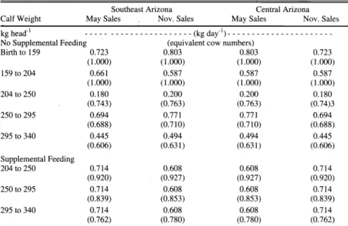
Table

¹

shows the average daily gains

estimated for different sale weights and

dates by region plus the equivalent cow

numbers that can be maintained for each

scenario. Rates of gain for the 2 regions

were set up to mirror each other with the

Table 1. ADG (kg day

¹⁾

and equivalent cow numbersa.

Southeast Arizona Central Arizona

Calf Weight May Sales Nov. Sales May Sales Nov. Sales

kghead' --- ---(kgday')---

No Supplemental Feeding (equivalent cow numbers)

Birth to

159

0.723 0.803 0.803 0.723

(1.000) (1.000) (1.000)

159

to 204 0.661 0.587

(1.000) (1.000) (1.000)

204 to 250 0.180 0.200

(0.743) (0.763) (0.763)

250 to

295

0.694

0.771

(0.688) (0.710) (0.710)

295

to 340 0.445 0.494

(0.606) (0.631) (0.631)

Supplemental Feeding

204 to 250 0.714

(0.920) (0.927) (0.927)

250 to 295 0.714 0.608

(0.839) (0.853) (0.853)

295 to 340

0.714 0.608

(0.762) (0.780) (0.780)

aEquivalent

cow numbers in parentheses were obtained by reducing available Animal Unit Years for cows by 0.5, 0.6, and 0.7 for the number of days it took calves that would be sold to go from 204 to 250, 250 to 295, and 295 to 340 kg head'; respectively. No distinction was made for weights less than 204 since these calves always reached their weight before

8

months of age, within the normal bounds of a one-year breeding and calving cycle.

most favorable gains occurring prior to November and May sales for the southeast and central regions. The most favorable forage conditions under supplementation assume a growth rate of 0.803 kg day' for weights from birth to 159 kg and 0.794 kg day

¹

for weights from 204 to 340 kg head-'.

These rates of gain were reduced by 10%

when forage is less abundant in each region prior to the animal's sale date.

These growth rate assumptions and the 10% reduction applied when forage is less abundant were derived from conversations with University of Arizona colleagues and Arizona ranchers. To calculate the cows that could be supported on an Animal Unit Year (AUY) of forage, reductions of 0.5, 0.6, and 0.7 AUYs were charged for the number of days it took calves to go from 204 to 250, 250 to 295, and 295 to 340 kgs, respectively. For example if it took 180 days for a calf to go from 204 kg to 250 kg, the AUY reduction would be 0.5*(180/365), where 0.5 is the assumed Animal Unit equivalency for this average calf weight. The AUY reduction for pro- ducing calves heavier than ^{204 kg} head

¹

has the effect of reducing total cow num- bers and thereby reducing the number of calves available for sale. No opportunity cost of fewer cows is added when going from 159 to 204 kg sale weights since 204 kg calves are weaned at about 7 months of age, which allows ample time for cows to breed back in a year-round calving system.

Birth dates and supplement require-

ments to meet the daily rates of gain in Table

¹

are described in Table 2. Birth dates were calculated working backwards from the sale date and the corresponding rate of gain for each protocol. The amount of supplement required is dependent upon sale weight, sale date, and region. Prior to weaning, calves less than 204 kg head'

consume little forage so that supplemental feeding was only considered for calves above this weight level. The amount of supplement fed ranged from 45 to 181 kg AU', varying in average annual cost from

$10.31 to $41.23 AU'. The cost ($Ikg) of a 50:50 corn meal and cottonseed meal mixture was charged using Arizona corn

meal and cottonseed feed costs for the quarter fed as reported by U.S.

Department of Agriculture, Agricultural Prices (1980-1998). Because some ranch- ers may be able to obtain more of a whole- sale than retail price for supplement, we did not charge additional labor or fuel expenses for distributing supplement to the cow herd. However, the distribution costs for supplement may be very impor- tant, depending on the terrain of the ranch.

Another expense item that varied with different sale date and weight options was the opportunity cost of sale. That is, calves sold at 204 kg could have been sold at 159 kg and so forth. The opportunity cost of funds was charged at a real annual interest rate of 4%. All other cost items except for grazing expenses were obtained from Economic Research Service's cow-calf production costs for the West (USDA 1982-1998). Cash grazing costs were cal- culated using the grazing fees and accom- panying percentages of grazing land in

Arizona owned by the State (33%), Bureau of Land Management (17%), Forest Service (40%), or Private entity (9%) as reported in Mayes and Archer (1982). Common variable and fixed cash expenses for all sale weight and date com- binations are available in Tronstad et al.

(2001). Gao (1996) also provides more detail about the cost items incorporated.

Cull cows were assumed to weigh 454 kg head', irrespective of the herd's mix or production protocol. In addition, a calf crop percentage of 80% per exposed cow, calf death loss after birth of 2.5%, and a

culling percentage of 16% with a 4%

annual death loss for cows was applied to all scenarios. The calf crop percentage of 80% per exposed cow falls within the range of values given in Teegerstrom and Tronstad (2000). Calf and cow death loss- Table 2. Supplement requirements and calculated birth dates by sale date, sale weight, and loca-

tion.

Calving Date Supplement Required

SE AZ Central AZ 50:50 Corn & Cottonseed Meal Ration

May Sales Nov. Sales Sale Weight

27 Nov. 30 May

(kg head')

159

head') pair')

21 Sept. 24 Mar. 204

19 July 19 Jan. 250

0

17 May 17 Nov. 295

14 Mar. 14 Sept. 340

Nov. Sales 16 June

May Sales 14 Dec.

16 April 14 Oct. 204

18 Feb. 18 Aug. 250

0

23 Dec. 22 June 295

0

27 Oct. 26 April 340

⁰

Note: Expert opinion was used to determine the supplement requirements needed to attain the ADG rates described in Table

1.

JOURNAL OF RANGE MANAGEMENT 56(5) September 2003 427

Table 3. Range calf growth model and corresponding parameter estimates.

Variables Description

Constant Age;

Aged

Age31 Age4i Age;' Age6i Age73 Age8!

o equals estimated birth weight (kg head). Age1 i indicates age of calf i in months at the/h weighing for each of the corresponding

8`h

order polynomial terms.

Polynomial order associated with the age growth function was determined by applying the Schwartz (1978) criteria of estimating

8

WT;,1 as a function of Z $; Agea1.

u=

Corresponding Parameter t-values Parameters Estimates

DHt Dummy variable that is

¹

if heifer and 0 if steer.

(wT;,1- GFRS;,I) (WT;,2 - ^GFRS;,2)

(WT;,3 - ^GFRS;3)

(WT;.4 - GFRS;.4)

Impact of the difference in animal is weight at their prior weighing versus that expected by

GFRS;, f_I at thejh weighing (j=2,3,4, and

⁵

or the 3, 8, 12, and 20-month weighings, respectively.)

CGtao Compensatory gain effect at the 20-month weighing for animal i.

Rain?i3 Centimeters of rainfall from the j-1 to j ^month

Rainy ^4'4 weighing in a given year less the 30-year-average Raintj'S rainfall for these same months (j = 3, 4, and 5).

I3o

37.143 52.277

13I

96.924 13.246

12 -65.850 -9.509

f3 22.565 9.384

134

-3.806 -9.106

f5 ^{0.345 8.569}

16 -0.172E-01 -7.890

/3

0.446E-03 7.169

$s -0.470E-05 -6.467

8;, -0.497E-01 -10.344

8w2

0.534 2.120

8w3

0.274E-01 1.839

6w4 0.406 28.269

5w5

0.763 35.872

8CG -0.497E-01 -5.868

8r3 2.001 17.120

Sr4 0.727 11.378

8r5 0.614E-01 0.375 D! Dummy variable that is

¹

if it is the jth weighing or 0 otherwise.

Notes: Refer to equations I through 3 for a formal description of the variables and model estimated. The

model's

adjusted R-squared was 0.941 and standard errors used to obtain t-ratios were calculated using the Robust White procedure, using ^TSPTM v4.5.

es are mid-range to those reported by Tronstad and Gum (1994). The calf crop is assumed to be a 50:50 mix of steers and heifers. For a 100-AU ranch selling 159 or 204 kg calves, a total of 100 cows plus 20 heifers are exposed to the bull every year.

The combined weight of heifer calves selected as replacements at weaning plus bred heifers will exceed the average weight of the 80-cow AUYs in the herd.

But cows may die throughout the year and not just at weaning, offsetting the larger grazing needs of the combined heifer calf and bred heifer AUYs. Irrespective, the same heifer development costs are equally imputed for all scenarios. Out of the 100 cows, 16 are culled and 4 are expected to die. The 80% assumed fertility results in 96 calves born and the 2.5% calf death loss results in 93.6 calves at weaning. To replenish the cows that are culled or die, 42.7% (20/46.8) of all heifers are retained each year as replacements with 80% fertil- ity. Thus, a 100-AU ranch selling 159 kg or 204 kg calves would expect to sell 16.0 cows, 46.8 steer calves (i.e.,120*0.8*0.975*0.5), and 26.8 heifer calves annually.

founds pr hl

I,

Results

Calf weights were estimated as a func- tion of age, sex, climate, calf weights at the previous weighing relative to an expected weight, and a 20-month compen- satory gain as described in equation (1).

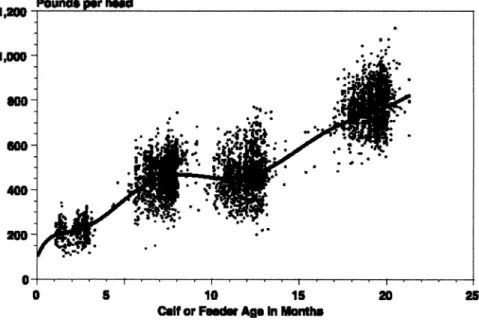
Table 3 provides the parameter estimates and corresponding statistics for this model. Note that the model to estimate calf weights is constructed so that if cli- mate and prior calf weights have been at their norms, weight is simply an ^8th order polynomial function of calf age in months with a constant weight percentage differ- ential between steers and heifers. Figure

1

graphically describes this polynomial growth function for a steer calf from birth to 20 months of age as plotted against the actual calf weight data. Estimated calf weights from equation (1) are presented in Figure 2. Unlike logistical growth func- tions, the polynomial framework has flexi- bility to allow for the dip in calf weight that occurs from weaning and seasonal forage availability. An ^8th order polynomi- al was selected from polynomial orders of

3 to 10 that were estimated, applying the Schwarz (1978) criteria to calf weight esti- mated as only a function of calf age. On average, calf weights at the 12-month weighing were 3.84 kg head

¹

less than at the 8-month weighing. At any given age, heifer calves were estimated to weigh 2.25 kg head

^t

less than a steer calf.

D 15

Alit or Fair ^{Age In Months 20}

Fig, 1. Calf scale weights and estimated polynomial age growth function for steer calves.

1,200 Pounds per hied

1,000-

mo

600-

5

M

10 15 20 2

tell or Fir ^{A90 In Months}

Fig. 2. Modeled calf weights based on equation 1.

If rainfall is above (below) the 30-year average for the months prior to a weigh- ing, calves would be expected to weigh more (less) than otherwise at their current weighing. Rainfall between the prior and current weighing is used as a proxy to estimate forage conditions being above or below their long-term average. As indicat- ed by the estimated rainfall parameters (Table 3), if the accumulated rainfall between the 3- and 8-month weighings was above the 30-year average by

1

cm, calves were estimated to weigh 2 kg head' more at the 8-month weighing than if rain- fall was equal to the 30-year average. The magnitude and statistical significance of the rainfall variable decreases as the ani- mal increases in age. This result is attrib- uted to the 20-month compensatory gain

region was a 250 kg sale weight with a production protocol of May sales and sup- plemental feeding. Supplemental feeding is more attractive for the central than southeast region because May sales have the most favorable rate of gain for the cen- tral Arizona region. The return in going for the 250 kg head' May sale weight feeding supplement is only $4.30 AUY' or 3.6% higher than the lighter 204 kg head' weight class, but an impact in fertil- ity would likely increase the return from feeding supplement as described below.

While the returns associated with the heaviest 2 sale weights of 295 and 340 kg

head' are consistently low, the risks or

standard deviations associated with these weights are generally lower as well. The highest 2 weight classes of 295 and 340 kg head' have a standard deviation that ^is on average 19% less than the more profitable lighter sale weights. However, the highest standard deviation of returns is also from feeding supplement and selling 340 kg head' feeders in the southeast region dur- ing November. Feeding large quantities of supplement adds a cost that significantly decreases profitability when the price of heavy feeders is low. However, supple- mental feeding can really boost revenues by bringing more calves and weight to market when prices for heavier feeders are strong in the fall. Combined cost and sea- sonal market forces make this production and marketing protocol the most risky.

While cull cow sales make up only 20%

to 23% of total revenues, they account for the largest share of the profit differential between May and November sales. Of the

$17.14 profit difference between May and November sales for 204 kg calves from southeast Arizona not fed supplement, cull cow sales account for 52% of the favor- able revenue difference between these months. Steer and heifer calf sales account for 33% and 15% of the favorable May sale revenue difference. For 250 kg sale weights from the central region feeding supplement, cull cow sales account for 46% of the favorable difference in May over November revenues, while steer and heifer sales account for only 37% and 17%

of this difference. However, if cull cow weights for a ranch are less for May than November instead of being equal as Table 4. Average 1999 real return and standard deviations of returns, ^($ AUY-1),1980-98.

effect and the greater importance of

lagged weight components as the animal Southeast Arizona Central Arizona

these factors Sale Weight May Sales Nov. Sales May Sales Nov. Sales

increases in a e g

^.

That is

,

were able to better capture both genetic and environmental components as the calves increased in age compared to the rainfall variable.

i ng t h i g ⁱ ns est i mate U s e we h t ga d a b ove Cattle-Fax (1981-1998) prices for calf and cow sales, and the opportunity cost of for- age described in Table 1(i.e., reduced cow numbers for heavier calf weights), the average and standard deviation of 1999 real returns for different sale dates and weights is given in Table 4. A sale weight of 204 kg head' for May with no supple- mental feeding is the most profitable alter- native for the southeast Arizona region.

An average real return of $120.45 AUY' for the southeast was realized for the 19 years from 1980 to 1998. The most prof- itable scenario for the central Arizona

(kghead"') ---

No Supplemental Feeding

($AUY')---

159

204

63.94 (67.04) 120.45

(62.38) 103.31

(67.11) 121.09

(62.32) 102.68

(73.80) (69.58) (73.92)

250 23.86 25.53

(54.01) (54.21) (56.66)

295 4.07 18.43

(49.52) (53.20) (53.12)

340 -62.06 -31.89

(39.09) (44.42) (44.25)

Supplemental Feeding

250 110.68

(73.22) (71.58) (74.10)

295 89.75 100.92

(69.95) (72.87) (71.73)

340

57.11 85.11

(66.56) (93.18) (69.53) (68.91)

aThe

sample standard deviation of returns is in parentheses below the average of annual real returns.

JOURNAL OF RANGE MANAGEMENT 56(5) September 2003 429

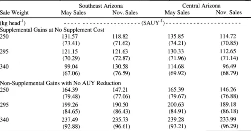
Table 5. Average 1999 real return and standard deviations of returns ($ AUY"1) for extra grass year scenarios, 1980-98.

Sale Weight

Southeast Arizona May Sales Nov. Sales

Central Arizona May Sales Nov. Sales (kghead') --- ---($AUY')---

Supplemental Gains at No Supplement Cost

250

131.57 118.82

(73.41) (71.62) (74.21)

295 121.15 121.63

(70.29) (72.87) (71.96)

340

99.04 130.58

(67.06) (76.59) (69.92)

Non-Supplemental Gains with No AUY Reduction

250

164.39 147.21

(79.48) (77.06) (79.67)

295

199.26 190.50

(84.65) (86.43) (84.91)

340

237.49 235.73

(92.88) (96.61) (93.21)

he sample standard deviation of returns is in parentheses below average annual real returns.

assumed, this would diminish the favor- able revenue difference of May over November cull cow sales.

Without feeding supplement, the esti- mated polynomial age growth function is essentially flat after reaching 7 months of age or 204 kg head' for the next 5.5 months. However, supplemental feeding is able to remove the long flat period for range calves from 7 to 12.5 months of age.

Feeding supplement at the level described in Table 2 to attain the accompanying Average Daily Gains (ADGs) described in Table

¹

increases average AUY' prof- itability for 250 kg calves sold in May by

$86.82 and $86.49 for the southeast and central regions, respectively. Even though supplemental feeding is not always the most profitable option, it consistently increases the return for sale weights above 204 kg head', anywhere from $83 to $119 AUY'.

Table 5 illustrates what the return to dif- ferent sale weights and dates would be if a rancher had "extra grass" so that supple- mental gains were obtainable without feeding supplement or no reduction in AUYs was charged for selling calves at heavier weights. These values are to pro- vide an illustrative benchmark that can be used to interpolate an abundant forage sit- uation rather than suggest that supplemen- tal gains or no AUY reduction will be attained in an "extra grass" year. Even when supplemental gains are available at no extra feed cost, 250 kg head' sales are the most profitable except for November sales in the southeast region. In general, the opportunity cost associated with fore- gone calf numbers and lower prices does not outweigh the benefit of heavier calf

weights, even when supplemental gains are imposed with no added feed cost. But if no AUY reduction is charged for pro- ducing heavier calves, the heaviest calf weight of 340 kg head' yields the highest return with May sales still somewhat pre- ferred over November sales for both regions.

While supplemental feeding removes the long flat growth period for range calves, it may also have an impact on fer- tility of the herd. The value ^($ AUY') of a 1% increase in fertility associated with feeding supplement is given in Table 6,

utilizing the supplemental ADGs described in Table 1. The value of a 1%

increase in fertility is about $5.50 AUY' for all supplemental fed sales. Using the returns given in Table 4, it would take an increase in fertility from feeding supple- ment of more than 1.78% ((120.45- 110.68)/5.49) before it would be more profitable to sell calves at 250 rather than 204 kg head' for May sales in southeast Arizona. Because supplemental feeding and May sales of 250 kg head' is the most profitable option for the central Arizona

region, fertility would have to decline by -0.78% ((121.09-125.39)/5.53) before ^it would not pay to feed supplement and increase the May sale weight from 204 to 250 kg head'. The value of a 1% increase in fertility accompanied with supplemental feeding is about the same for all sale weight categories because the supplemental fed rates of gain described in Table

¹

are roughly the same for all calves above 204 kg head'.

Discussion and Conclusions

This study shows that the benefit of higher sale weights was not enough to overcome lower calf prices and fewer calf and cull cow sales for calf weights above 204 kg head-' without feeding supplement.

Supplemental feeding removes the nearly 0

rate of gain for calves from 7 to 12.5 months of age, so that for the central Arizona region 250 kg head' calf sales in May fed supplement ^is the most profitable option. May sales were found to be more profitable than November sales, even with lower ADG rates. More favorable market conditions for May than November sales are the main reason why May sales were often more profitable than November sales.

In calculating cost and return estimates for cow-calf ranches in Arizona, Teegerstrom and Tronstad (2000) con- ducted focus groups in ⁵ different regions to gain insights into typical production practices. They reported a typical sale weight for steers of between 204 to 250 kg head', depending on the ranching region.

This result is consistent with the most profitable sale weight category of 204 kg head' for the southeast and 250 kg head' for the central Arizona regions. With regards to sale date, a fair number of ranchers market their calves in the fall rather than the spring, and May was deter- mined as the most profitable sale time for both regions. Given that the difference in profitability between May and November

Table 6. Value of a 1% increase in fertilitys associated with supplemental feeding.

Southeast Region Region Central Region

Sale Weight Category Mid-May Mid-Nov. Mid-May

(kg head') $AUY'

250

$

5.49

$

5.40

$

5.53 5.36

295

$

5.52

$

5.60

$

5.62

5.51

340

$

5.40

$

5.46

$

5.59 5.46

aFor fertility changes up to 85.5% after the increase and starting with an initial fertility rate above 34.2%. Given a 100

AUY ranch with fertility rates above 85.5%, bred cows will need to be sold or less than 20 heifer calves will need to be

retained for breeding to keep the herd at a constant AUY. Fertility rates below 34.2% are unable to sustain the cow herd

even with 100% of the heifer calves retained for breeding. Value of fertility utilizes the ADGs associated with feeding

supplement as described in Table

1.

sales was found to be relatively small in comparison to alternative sale weights, small differences in biological productivi- ty from what was assumed in this analysis could shift results to favor November sales, especially for the southeast Arizona region. In addition, rates of gain were adjusted from a calculated weight gain using expert opinion for fall and winter calving dates and changes in the values assumed could sway results. This indicates that formal studies on these relationships should be considered. High labor and dis- tribution costs to remote and difficulty in accessing range sites could also make sup- plemental feeding less attractive than what we have determined in our analysis.

However, each rancher can adjust the return values presented to fit their own cost and production values in evaluating alternative sale dates and weights.

It is also important to note that a more flexible sale date, weight combination, and supplemental feeding strategy could have generated more net return than the "fixed strategies" above. For example, a strategy that can take advantage of market opportu- nities for feeding calves to a heavier weight when corn prices are high and for- age is available would outperform the best

"fixed strategies" presented of always pro- ducing 204 or 250 kg calves for sale in May. That is, when corn prices are so high that heavier calves sell for a higher price

kg' than light calves, a rancher benefits from both the higher price received and more kgs sold by keeping calves until they are at a heavier weight class.

Literature Cited

Cattle-Fax. 1981-1998. Cattle-fax feeder cattle cash prices for Arizona.

Clayton, H.L., R.P. Morris, and J.R. Wight.

1983. Using precipitation to predict range herbage production in Southwestern Idaho. J.

Range Manage. 36:766-770.

Fox, D.G. and J.R. Black. 1977. A system for predicting performance of growing and fin- ishing cattle. 1. Development of a model to describe energy and protein requirements and feed values. Feedstuffs 49:21-22, 27.

Gao, X.1996. An evaluation of hedging strate- gies for alternative sale dates and weights.

M.S. Thesis, Univ. Arizona, Tucson, Ariz.

Lambert, D.K. 1989. Calf retention and pro- duction decisions over time. W. J. Agr. Econ.

14:9-19.

Mayes, H.M. and T.F. Archer. 1982. Arizona cattle ranches on public land. Univ. Arizona, College of Agr. Range Task Force Rep.

Tucson, Ariz.

Schwarz, G. 1978. Estimating the dimension of a model. Ann. Statist. 6:461-464.

Sprinkle, J.E. 2000. Managing nutritional challenges to reproduction. Univ. of Arizona Coop. Exten. Publ. AZ1166, Tucson, Ariz.

Teegerstrom, T. and R. Tronstad. 2000. Cost and return estimates for cow/calf ranches in five regions of Arizona. Univ. of Arizona Coop. Exten. Publ. AZ1193, Tucson, Ariz.

Tess, M.W. and B.W. Kolstad. 2000.

Simulation of cow-calf production systems in a range environment: I. Model Evaluation. J.

Anim. Sci. 78:1170-1180.

Tronstad, R. and R. Gum. 1994. Cow culling decisions adapted for management with CART. Amer. J. Agr. Econ. 76:237-249.

Tronstad, R., T. Teegerstrom, and X. Gao.

2001. Trade-off between cow numbers, calf size, and sale date incorporating seasonal factors and supplemental feeding: Ranch Business Management. _pp. 181-187 In:

Tronstad, R., J. Sprinkle, and G. Ruyle (ed.), Arizona Ranchers' Management Guide.

Univ. of Arizona Coop. Exten. Publ.

AZ1279, Tucson, Ariz.

TSP 1999. User Manual Version 4.5 TSP International, Palo Alto, Calif.

U.S. Department of Agriculture. 1980-1998.

Agricultural Prices. National Agr. Stat.

Serv., Agr. Stat. Board, Washington D.C., recent data available at http://usda.

mannlib.cornell.edu/reports/nassr/price/pap-bbl (last accessed August 2002)..

U.S. Department of Agriculture. 1982-1998.

Cow-calf production cash costs and returns.

Econ. Research Serv., Washington D.C., recent data available at

http://www.ers.usda.gov/Data/CostSAnd Returns/testpick.htm (last accessed August 2002).

Van Tassell, L.W., R.K. Heitschmidt, and R.J. Conner. 1987. Modeling variation in range calf growth under conditions of envi- ronmental uncertainty. J. Range Manage.

40:310-314.

Western Regional Climate Center.

1961-1998. Monthly total precipitation for San Carlos reservoir, Arizona, available at http://www.wrcc.dri.edu/summary/clims- maz.html (last accessed August 2002).

JOURNAL OF RANGE MANAGEMENT 56(5) September 2003 431