Munich Personal RePEc Archive
The Risk Spiral: The Effects of Bank
Capital and Diversification on Risk
Taking
Peleg Lazar, Sharon and Raviv, Alon
Tel Aviv University, Bar Ilan University
February 2019
Online at
https://mpra.ub.uni-muenchen.de/92134/
The Risk Spiral: The Effects of Bank Capital
and Diversification on Risk Taking
∗
Sharon Peleg Lazar
Tel Aviv University
Alon Raviv
Bar Ilan University
Feb 2019
Abstract
We present a model where bank assets are a portfolio of risky debt claims and
analyze stockholders’ risk-taking behavior while considering the strategic interaction
between debtors and creditors. We find that: (1) as the leverage of a bank increases,
risk shifting by borrowers increases, even if their leverage is unchanged (zombie
lend-ing). (2) While the literature demonstrates that an increase in the co-movement of a
loan portfolio increases the bank’s cost of default directly, we find that the increase
in co-movement causes an increase in risk shifting that further increases the cost of
default (3) Risk shifting decreases with the diversification of a loan portfolio.
Keywords: Risk taking, Banks, Comovements, Deposit insurance, Zombie lending
JEL Classification: G21, G28, G32, G38
∗Peleg Lazar: Coller School of Management, Tel Aviv University, Tel Aviv, Israel,
1
Introduction
The contingent claim approach to analyzing bank risk assumes that the value of bank assets follows a geometric Brownian motion. Hence, the value of the bank stock can be replicated
by a call option on the value of its assets, similarly the value of deposit insurance can be
replicated by a put option on the bank’s assets (Merton, 1977; Ronn and Verma, 1986; Laeven and Levine, 2009; Beltratti and Stulz, 2012). However, the approach does not consider three
important aspects of bank assets. First, commercial bank assets are often in the form of
debt – loans and bonds – with a limited upside (Dermine and Lajeri, 2001; Gornall and Strebulaev, 2018; Nagel and Purnanandam, 2015). Second, bank assets are composed of a
portfolio of loans to different borrowers with varying leverage, asset risk, and asset correlation
(Flannery, 1989; Chen, Ju, Mazumdar, and Verma, 2006). Third, a bank can increase its
level of asset risk in a way that shifts value to its stockholder at the expense of its debtholders and depositors, i.e., engage in risk shifting (Jensen and Meckling, 1976; Galai and Masulis,
1976). To our knowledge, this paper is the first to consider all three elements of bank assets
simultaneously when analyzing a bank’s motivation to monitor its borrowers’ risk.
We assume that a bank’s assets are a portfolio of loans to corporations. The borrowers’
assets, which serve as collateral for the loans, follow a geometric Brownian motion (Gornall
and Strebulaev, 2018; Nagel and Purnanandam, 2015). Due to the legal limited liability of stockholders, a borrower’s stock value has a lower limit of zero. Thus, a borrower’s stock
value is a convex function of its asset value and can be analyzed as a call option on the
corporation’s asset value (Merton, 1974). By contrast, since bank assets have a limited upside, where the limit is equal to the sum of the face values of all loans, the value of a
bank’s stock has both a lower and an upper limit.
Based on the above assumptions regarding bank assets, we develop a pricing model for the liabilities of a bank and of its borrowers and analyze the equilibrium levels of asset risk
and limiting the risk of their borrowers, we assume that borrowers can increase their level of
asset risk from its initial level only with the consent of the bank.1 By contrast, the ability
of a bank’s creditors to limit bank risk shifting is restricted, thereby bank’s stockholder can change the level of asset risk.2 Once we determine whether both the stockholder of the bank
and the stockholders of the borrowers are better off shifting asset risk, we characterize the
equilibrium level of risk of each borrower. Our model allows us to find the bank’s monitoring
policy for each individual borrower, given the leverage ratio of that borrower and the leverage of the remainder of the bank’s loan portfolio.
We show that when a borrower is solvent, i.e., its asset value is above the face value
of its debt, the stockholder of the bank monitors the borrower’s asset risk closely, thereby preventing any increase in risk. This result does not depend on the leverage ratio of the bank
or on the correlation between the asset returns of the bank’s borrowers. By contrast, we
demonstrate that when a borrower is insolvent, i.e., its asset value is below the face value of its debt, the equilibrium level of asset risk increases with the borrower’s leverage, motivating
the bank to reduce its monitoring effort and allow the borrower to increase risk.
The major contribution of our analysis relates to the cross-borrower effect on the equi-librium asset risk of a borrower. Specifically, we demonstrate that if a borrower is insolvent,
its equilibrium level of asset risk increases with the leverage ratio of the other borrowers.
Put differently, as a bank’s capital ratio decreases, its stockholder is motivated to allow an insolvent borrower to increase risk, even if that borrower’s own leverage ratio is unchanged.
This result is in line with banks exhibiting “zombie lending” behavior where
undercapital-ized banks are found to prefer existing low-quality borrowers to existing or new high-quality borrowers, as described in Acharya, Eisert, Eufinger, and Hirsch (2016), Schivardi, Sette,
and Tabellini (2017), Giannetti and Simonov (2013), and Peek and Rosengren (2005). By
1
Brealey, Leland, and Pyle (1977), Campbel and Kracaw (1980), Diamond (1984), Fama (1985).
2
contrast, well-capitalized banks are not found to exhibit this behavior.
Studying the effect of deterioration in bank capital on a bank’s risk-taking motivation
challenges the empirical literature due to the difficulty in identifying the causal impact of bank capital shocks on risk taking. A growing literature uses loan-level data to overcome
this identification problem (Ioannidou, Ongena, and Peydr´o, 2014; Tracey, Schnittker, and
Sowerbutts, 2017; Ohlrogge, 2017). We address loan-level analysis by assuming that the
loans in a bank’s portfolio can have different weights. We find that for insolvent borrowers, as the weight of a loan in a bank portfolio increases the equilibrium level of risk for this loan
increases as well. Thus a study focused on the effect of a decrease in capital on marginal
loans would find a lower increase in risk than a study that focuses on the entire loan portfolio. The financial and economic literatures present ample evidence that in time of crisis
co-movement between the returns of assets increases (Das, Duffie, Kapadia, and Saita, 2007;
Duffie, Eckner, Horel, and Saita, 2009). This increase in the correlation between the returns of assets serving as loans’ collateral increases the volatility of bank assets and, as a result,
increases the value of the bank’s stock and its cost of default, while decreasing the value
of its debt (Gornall and Strebulaev, 2018).3 We show that the above-mentioned increase in comovement can affect the cost of default through a second channel: its positive impact on
the stockholders’ risk-taking motivation. Consequently, the bank’s cost of default and the
value of its equity increase further while the value of bank assets and debt decrease.
Our paper relates to papers that (1) analyze bank asset as risky debt claims, (2) analyze
the cost of banks’ default and (3) the effect of risk shifting on the cost of default. Flannery
(1989) generalizes the traditional model for pricing deposit insurance, which assumes a bank with a single asset (Merton, 1977; Marcus and Shaked, 1984; Ronn and Verma, 1986), to
the case of a bank with a diversified portfolio of assets. However, Flannery’s model ignores
3
the special nature of bank assets as risky debt claims, and instead assumes that each asset
follows a geometric Brownian motion. Dermine and Lajeri (2001) analyze the cost of deposit
insurance while accounting for the nature of bank assets as risky debt claims. Their model assumes a bank with a single borrower whose assets follow a geometric Brownian motion.
The authors present closed-form solutions for the values of bank debt, equity, and deposit
insurance and show that ignoring the nature of bank assets as risky debt claims results in an
underestimation of the cost of deposit insurance. Chen, Ju, Mazumdar, and Verma (2006) build on the work of both Dermine and Lajeri (2001) and Flannery (1989) and analyze the
cost of deposit insurance in a model where bank assets are a diversified portfolio of risky
debt claims. However, in both papers, unlike our paper, asset risk is exogenous and not a result of a strategic interaction between claimholders.
Peleg Lazar and Raviv (2017) study the motivation of a bank’s stockholder to increase
risk when bank assets are composed of a single risky loan, in a setting similar to the one used by Dermine and Lajeri (2001). The authors find that a bank’s stockholder is motivated
to shift risk only when the borrower is insolvent and the bank itself is insolvent or near
insolvency. In contrast, in the current paper, we analyze the effect of diversification and the motivation of a bank to shift risk with respect to the entire loan portfolio of the bank.
The rest of the paper is organized as follows. The liability structure of the bank and
of its borrowers and their valuations are presented in Section 2. An equilibrium model for the level of borrowers’ asset risk is defined in Section 3. Section 4 includes a quantitative
analysis of the model’s results. Section 5 concludes.
2
Liability Structure and Valuation
In this section we describe the liability structure of both the bank and its borrowers, express
different corporate claims in order to find the equilibrium levels of risk of the bank’s borrowers
and the equilibrium value of these claims, as presented in section 3.
2.1
The liabilities structure of the corporations
There are N corporations, each funded by equity with a market value of Si,t (where i ∈
{1, ..., N}), and a single loan with a face value of Fi, and a market value of Bi,t. The loan
is a zero-coupon loan maturing at time T and the bank is the single creditor. The value of each corporation’s assets, Vi,t, follows a geometric Brownian motion according to the
following equation:
dVi,t =µiVi,tdt+σiVi,tdWi,t, (1)
where µi is the instantaneous expected return on the corporation’s assets, σi is the
instan-taneous volatility of the corporation’s assets, and dWi,t is a standard Wiener process. We
denote by ρi,j the instantaneous correlation coefficient between the standard Wiener
pro-cesses of any two corporations,4 E(dW
idWj) = ρi,j, where i, j ∈ {1, ..., N} and i 6= j. The
value of each of the corporations’ assets, Vi,t, can be viewed as the loan’s collateral.
Corporation i defaults at debt maturity, T, if the value of its assets, Vi,T, is lower than
the face value of its debt, Fi. In this case, the creditor takes over the corporation and
receives the residual assets of the corporation,Vi,T. Otherwise, the debt is fully paid and the
creditor, the bank, receives the entire face value of the debt,Fi. Therefore, the payoff to the
corporation’s debtholder can be expressed as Bi,T = min(Vi,T, Fi), which can be restated as
Bi,T =Fi−max(Fi−Vi,T,0).
As developed by Merton (1974), this payoff is equivalent to the payoff of a risk-free debt
minus a European put option. Thus, the present value of the loan is given by:
4
Assuming equal pairwise correlations, ρi,j =ρ for alli and j such that i 6= j, and following Vasicek
(2002), we can representdWi as dWi =√ρdY +√1−ρdZi, where dY and dZi are independent standard
normal variables. In such a case, Y can be interpreted as a common factor whiledZi can be interpreted as
Bi,t =Fie−r(T−t)−P utt(Vi,t, Fi, σi, T −t), (2)
wherer is the risk-free rate andP utt(Vi,t, Fi, σi, T −t) is the price of a European put option
on the asset value of the corporation, at timet, with a strike price equal to the face value of its debtFi, asset risk σi, and time to maturityT −t.
Since the equity is the residual claim, its payoff at debt maturity isSi,T = max (Vi,T −Fi,0).
Consequently, the value of the corporation’s stock can be replicated by a European call
op-tion on the value of the corporaop-tion’s assets, with a strike price equal to its face value of debt (Galai and Masulis, 1976):
Si,t =Callt(Vi,t, Fi, σi, T −t), (3)
where Callt(Vi,t, Fi, σi, T −t) is the price of a European call option on the asset value of
corporation i, at time t, with a strike price equal to the face value of its debt Fi, asset risk
σi, and time to maturity T −t.
2.2
The bank’s liability structure
The bank is funded by equity with a market value of SB,t and a zero-coupon debt with a
face value of FB and a market value of BB,t. As discussed in Marcus and Shaked (1984)
and Ronn and Verma (1986), due to the periodic frequency of auditing, bank deposits are
analogous to a debt claim which matures on the date of the next audit, which we assume to
be T.
Since the bank’s assets are a portfolio of loans, as described in Section 2.1, we can express
the value of the bank’s assets at debt maturity as:
VB,T = N
X
i=1
Bi,T = N
X
i=1
To explore the effect of the size of a loan on risk-taking motivation, we rewrite equation
4 in terms of portfolio weights by defining wi as the weight of the loan to borrower i out of
the bank’s entire portfolio, wi ≡ Fi/Fp, where FP is the sum of the face values of all loans
in the bank’s portfolio, FP ≡ N
P
i=1
Fi. Now equation 4 can be expressed as:
VB,T = N
X
i=1
[wiFP −max(wiFP −Vi,T,0)]. (5)
The discounted value of the bank’s assets at any time prior to debt’s maturity is given
by:
VB,t = N
X
i=1
e−r(T−t)F
i− N
X
i=1
P utt(Vi,t, Fi, σi, T −t). (6)
The debtholder’s payoff at maturity is the minimum between the value of the bank’s
assets, VB,T, and the face value of its debt,FB, and can be expressed as:
BB,T = min (VB,T, FB) = FB−max
"
FB− N
X
i=1
Fi+ N
X
i=1
max(Fi−Vi,T,0),0
#
. (7)
The value of the bank debt at any time prior to debt maturity is given by discounting
the future payoff:
BB,t =e−r(T−t)EtQ[BB,T], (8)
whereEtQ[.] denotes the conditional expectation under the risk-neutral measure Q, given the information available at timet. Thus the value of the bank’s debt can be found by simulating the distribution of BB,T as defined in equation 7.
As in Chen, Ju, Mazumdar, and Verma (2006), the value of the bank’s debt at time t
can be rewritten as:
BB,t =e−r(T−t)FB−Gt {Vi,t}Ni=1,{Fi}Ni=1,{σi}Ni=1, FB, r, T −t
where Gt is the value of a European put option on the bank’s aggregate asset value with
maturity T. The exercise price of the put option is the face value of the bank’s debt, FB.
Since the bank’s equity is the residual claim and has limited liability, its payoff at debt maturity is the maximum between zero and the difference between the value of the bank’s
assets and the total face value of its deposits: SB,T = max[VB,T −FB,0]. By substituting
the value of the bank assets VB,T with its payoff as expressed in equation 4, the stock payoff
can be expressed as:
SB,T =max
"
(
N
X
i=1
Fi)−FB− N
X
i=1
max(Fi−Vi,T,0),0
#
. (10)
If at debt maturity all borrowers are solvent the stockholder receives the maximum pos-sible payoff: (
N
P
i=1
Fi)−FB. As discussed in Chen, Ju, Mazumdar, and Verma (2006), this
differs from the basic structural approach in which the stockholder’s payoff is unbounded
from above.
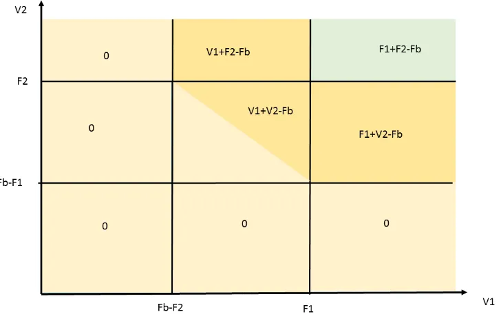
The payoff structure of the stockholder can be demonstrated in a simple example with
two borrowers (figure 1), where we sort this payoff into five different cases based on the
value of the borrowers’ assets. If both borrowers are solvent, F1 < V1,T and F2 < V2,T, the
bank stockholder receives the maximum payoff, (F1+F2)−FB. If borrower one is solvent,
F1 < V1,T, while borrower two is in default but its asset value is high enough to insure
depositors are paid back in full, (FB −F1) < V2,T < F2, then the payoff to the bank’s stockholder is positive, but below its maximal level and equals (F1 +V2,T)−FB. In this
state, the payoff is insensitive to changes in the asset value of borrower one, but sensitive to
changes in the asset value of borrower two. In the symmetrical case, where the asset value of borrower one is in the range of (FB −F2) < V1,T < F1, while borrower two is solvent,
F2 < V2,T, the bank stockholder’s payoff is (V1,T +F2)−FB. In this state, a change in the
are insolvent, V1,T < F1 and V2,T < F2, while the sum of their asset values is enough to pay depositors in full, FB <(V1,T +V2,T), the bank stockholder receives the residual payoff
(V1,T +V2,T)−FB. In this case, the payoff is sensitive to the asset value of both borrowers.
In the remaining case the bank stockholder receives no payoff.
We adjust equation 10, which presents the value of bank equity, to account for the weights
of the loans that compose the bank’s loan portfolio:
SB,T =max
"
(
N
X
i=1
wiFP)−FB− N
X
i=1
max(wiFP −Vi,T,0),0
#
. (11)
The value of the bank’s stock at any time prior to debt maturity can be expressed as:
SB,t =e−r(T−t)EtQ[SB,T], (12)
Since there is no closed-form solution to this equation, we solve it using Monte Carlo simu-lation.
2.3
The cost of deposit insurance
We assume that the bank’s deposits are insured by the government or a government agency.
The regulator conducts periodic audits to assess the solvency of the bank and to estimate its deposit insurance premium. At the time of an audit, the bank pays the fair insurance
premium according to its capital structure and risk. A change in the quality of the bank’s
loan portfolio between audits does not affect the risk premium that is charged from the bank for that period.5
If at debt maturity the value of the bank’s assets is below the face value of its deposits
5
the insurer compensates the depositors with the difference between the two. Thus, the cost
of deposit insurance equals the maximum between zero and the difference between the face
value of the secured deposits and the value of the bank’s assets. Using the expression for the bank’s assets payoff in equation 4, the payoff of the deposit insurance can be expressed as:
DIT =max(FB−VB,T,0) =max
"
FB− N
X
i=1
Fi+ N
X
i=1
max(Fi−Vi,T,0),0
#
. (13)
Therefore, the cost of the deposit insurance is given by:
DIt=e−r(T−t)EtQ[DIT]. (14)
The cost of deposit insurance per dollar of insured deposits, which we denote byDIP Dt,
is defined as the cost of deposit insurance divided by the face value of the bank’s debt, FB.
The cost of deposit insurance is interpreted as a proxy for the cost of bank default, which includes the real damage to the economy from a collapse of a large financial institution.
2.4
The probability of default
A default event occurs if the value of the bank’s assets is below the face value of its debt at
debt maturity. Therefore, the probability of bank default is given by:
P Dt =P r(VB,T < FB|Ft)
=P r
N
X
i=1
[wiFP −max(wiFP −Vi,T,0)]< FB|Ft
! (15)
where Ft denotes the information available at time t. As discussed in section 3, the
3
An Equilibrium Model For Risk Shifting
In this section, we describe our principal-agent model: the different claimholders’ strategies and incentives. We then define equilibrium in the setting of the model.
3.1
The framework of analysis
When the bank provides funds to a borrower in the form of a zero coupon loan, some initial
level of asset risk, σi,Initial, is realized.6 The face value of the borrower’s loan, Fi, is set
to account for this initial level of asset risk. Consequently, at the time that the loan is
initiated, the bank’s liabilities - stock and secured deposits - are fairly priced according to
the corporation’s asset risk and leverage. However, sometime after the contract is set, an
exogenous shock occurs to the asset value of one or more borrowers. The change in asset value alters the sensitivity of the bank’s equity value to asset risk. As a result, the bank’s
stockholder might be willing to tolerate a change in asset risk by one or more borrowers.
The strategic behavior of the bank and its borrowers that leads to equilibrium is based on the following observations. First, the empirical and theoretical literature suggests that banks
are effective in monitoring and limiting their borrowers risk shifting (Brealey, Leland, and
Pyle, 1977; Campbel and Kracaw, 1980; Diamond, 1984; Fama, 1985). Second, as discussed in the introduction, the ability of the bank’s creditors to prevent or limit risk shifting is
more restricted. Based on these stylized facts, we assume that the stockholder of the bank
maximizes the value of the bank’s stock regardless of the effect on the value of the bank’s debt, i.e., deposits. However, the stockholder of the bank does not control asset risk directly.
Instead, the borrowers’ stockholders are the ones that can actively shift the asset risk of
their firms. The borrowers, who are managed by equity-aligned managers would be willing to shift asset risk only if the value of their stock is positively affected by this shift.
The implications of these assumptions is that any change in the level of a borrower’s
6
asset risk requires the consent of the stockholders of both the bank and the borrower. More
specifically, the bank’s stockholder can set the boundaries for each borrower’s asset risk,
[σi,LBound, σi,U Bound], and the stockholder of the borrower can choose the level of asset risk
within this range. However, the bank cannot force a borrower to change its asset risk from
the initial level. A shift in the level of asset risk occurs only if the two counterparts, i.e., the
stockholder of the corporation and the stockholder of the bank, are better off.
The equilibrium is determined by a two-steps backward induction. First, the stockholder of each borrower chooses the level of asset risk,σ∗
i that maximizes the value of her stock, while
taking into account the upper and lower bounds of asset risk set by the bank’s stockholder:
σi ∈ [σi,LBound, σi,U Bound]. Since the bank cannot force a borrower to change risk from the
initial level, the domain of asset risk must contain the initial level of asset risk,σi,Initial. Next,
while taking into account the decision rule of the borrowers, the bank’s stockholder chooses
the upper and lower bounds of asset risk for each borrower,σ∗
i,LBound andσi,U Bound∗ . Since the
bank will tolerate a change in risk by a borrower only if its stockholder is better off, for any
σi ∈[σi,LBound, σi,U Bound] the value of the bank’s stock, SB,t, is greater than or equal to the
value of the bank’s stock under the initial level of asset risk. Bothσ∗
i,LBound andσi,U Bound∗ are
positive and the upper bound on asset risk is limited by the existing technologies governing
the borrower’ asset risk.
If the stockholders of the bank and the borrowers choose a strategy and none can ben-efit from changing it, then the set of strategies and corresponding payoffs, constitute a
Nash equilibrium. We define the set of parameters and payoffs in such an equilibrium as
{σ∗
i}Ni=1,{σi,LBound∗ }Ni=1,{σ∗i,U Bound}Ni=1
, S∗
B,{Si∗}Ni=1
.
The risk preference of the borrower’s stockholder The equity of a borrower can be
replicated by a call option on the value of the borrower’s assets. Since the value of a call
the stockholder of each borrowing corporation prefers the highest possible level of asset risk.
In fact, the positive sensitivity of the borrowers’ stock value to asset risk eliminates the
bank’s need to set a lower bound on asset risk σ∗
i,LBound.
The risk preference of the bank’s stockholder Since the bank holds a diversified
portfolio of loans, its stockholder maximizes the value of equity by controlling the asset risk
of each of the individual borrowers. Thus, the bank stockholder’s optimization problem can
formally be defined as:
{σimax} N
i=1 ≡arg max
{σi}Ni=1
SB,t {Fi}Ni=1, FB,{Vi,t}Ni=1,{σi}Ni=1,{ρi,j}i6=j
Subject to: σi ≥σi,Initial
(16)
To find the effect of a borrower’s leverage on a bank’s risk taking we define the quasi leverage ratio as in Merton (1974): LRi,t = (Fi/Vi,t)e−r(T−t). We can now express the bank
stockholder’s optimization problem in terms of the borrowers’ leverage:
{σmax i }
N
i=1 ≡arg max
{σi}Ni
=1
SB,t {LRi}Ni=1, FB,{σi}Ni=1,{ρi,j}i6=j
Subject to: σi ≥σi,Initial
(17)
The level of a borrower’s asset risk that maximizes the value of the bank equity, σmax i ,
does not depend solely on the borrower’s leverage. Instead, it depends on the leverage ratios
of all the other borrowers and the correlation between the returns of their assets. The study of these effects is at the center of our paper and is analyzed in detail in section 4.
When the value of a borrower’s asset is above the face value of its debt, Fi, there is
certainty that the borrower will be solvent at maturity if the loan’s collateral is invested in a risk-free asset. Therefore, the value of the bank’s equity is maximized when the borrower’s
asset risk is equal to zero, or at a low enough level of asset risk so there are no realizations
allowing a borrower to increase its asset risk above zero. When the asset value of the
borrower is below the face value of its debt, the position of the bank’s stockholder may be
hump-shaped with respect to the asset risk of the borrower.
3.2
The case of a bank with identical borrowers and perfect
cor-relation
We begin our analysis with a bank with identical borrowers i.e., borrowers with the same
leverage ratio and loan size, and a perfect positive correlation between the returns of the
borrowers’ assets. In doing so, we attain a better understanding of the case of a bank with a diversified portfolio of loans in several ways. First, this simple case has a closed-form
solution for the optimal level of asset risk that clarifies the effect of the borrower’s leverage
ratio and the bank’s capital structure on risk taking in equilibrium. Second, as will be shown throughout the paper, diversification reduces risk shifting and, consequently, the case of a
bank with borrowers that have assets with perfect positive correlation serves as an upper
bound for the effect of risk shifting on a bank’s liabilities and cost of default.
If all the borrowers of a bank have the same leverage ratio and the correlation between
the returns of their asset is equal to one, i.e., the returns have positive perfect correlation,
then there is no advantage to diversification and the portfolio is identical to a bank with a single loan as analyzed in Peleg Lazar and Raviv (2017). In this special case, we can express
the total face value of the borrowers’ loan as FC = N
P
i=1
Fi and handle the analysis exactly as
in the case of a bank with a single borrower.
In the case of a single borrower, since a bank’s assets consist of a single loan, the payoff
at maturity is bounded from above, and can be described as a portfolio of risk-free debt and
a put option on the borrower’s asset value with a strike price equal to the face value of the borrower’s debt. Similarly, the value of the bank’s debt can be replicated by a portfolio of
face value of debt (Dermine and Lajeri, 2001). The bank equity is economically equivalent
to subordinated debt, which can be replicated by a ‘bull spread’ strategy, as demonstrated
in figure 2.
The sensitivity of a bank’s equity value to the asset risk of its borrower can be divided
into two segments defined by a threshold of the borrower’s asset value:
V∗≡(FB N
X
i=1
Fi)
1
2e−r(T−t) ≡(FCFB) 1
2e−r(T−t), (18)
When the total value of the borrowers’ assets is above this threshold, which is equal to the
discounted geometric mean of the total face value of the borrowers’ debt and of the bank’s
debt, the value of the bank’s equity decreases with asset risk. Thus, the bank stockholder would not benefit from an increase in asset risk of the borrowers. However, when the total
value of the borrowers’ assets is below the threshold V∗, the value of equity is hump-shaped
with respect to their asset risk. Therefore, the value of the bank’s equity is maximized at some intermediate level of asset risk. If the level of asset risk that maximizes the bank’s
equity value is above the initial level of asset risk, both the stockholder of the borrower and
the bank would be better off by increasing the level of risk to this point. This occurs when the value of the bank’s assets is below the following threshold, which is defined analytically
by Peleg Lazar and Raviv (2017) for the case of a single borrower and expressed here for the
general case of N identical borrowers:
V∗∗ ≡(FB N
X
i=1
Fi)
1 2e−
r+σ2
2
(T−t)
≡(FCFB)
1 2e−
r+σ2
2
(T−t)
. (19)
According to equation (19), the occurrence of risk shifting depends not only on the
leverage ratio of the borrowers and of the bank, but also on the initial levels of asset risk. When the total value of the borrowers’ assets is below the threshold V∗∗, the asset risk of
the position of the bank’s stockholder. As presented in Appendix A, the level of risk for each
loan, σmax
i , is defined as:
σmax ≡arg max
σ {SB(FB, FC, VC)}=
s
1
T −t ln
FBFC
(VC)2
−2r (20)
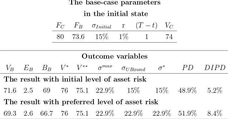
We illustrate risk shifting in the case of a bank with two identical borrowers with perfect
positive correlation using our base case parameters (table 1). As discussed in Section 2.2, all debt instruments mature at time T, which we assume is in one year,T −t= 1. In addition, we assume that the initial level of asset risk, σInitial, is 15%, in line with the asset risk of
corporations that issue investment grade bonds (Huang and Huang, 2012). The annual risk-free rate, r, is set to 1%. The face value of both borrowers’ debt is F1 = F2 = 40. Since the two borrowers are identical with a perfect positive correlation, this case is equivalent
of having a single loan, FC, with a face value of 80. We assume that the face value of the
bank’s debt is FB = 73.6, which yields a debt-to-asset ratio of 92% according to the bank’s
book-value.
We find that for any total value of assets below the threshold V∗ = 76 (equivalent to
bank leverage ratio of 95.9% based on market values), the level of asset risk that maximizes
the value of bank equity is strictly positive. Thus, risk shifting occurs only if the debtor’s
asset value is below this level. When the debtors’ initial level of asset risk is σInitial = 15%,
risk shifting occurs at any level of assets below V∗∗ = 75.1 (equivalent to a leverage ratio
of 96.2% based on market values). If, for example, the total value of the borrowers’ asset
declines to VC = 74, then the asset risk that maximizes the value of the bank equity is
σmax = 22.9% and the bank stockholder would allow the borrower to increase asset risk to
this level. Thus, the cost of deposit insurance per dollar of insured deposits increases from
4
Quantitative Analysis of Bank Risk Shifting
The analysis is executed in several steps. First, we analyze the bank stockholder’s preference for the asset risk of each of the borrowers. Next, we analyze the interaction between the
stockholders of the bank and of the different borrowers, when setting the level of asset risk in
equilibrium. Finally, we consider the effects of risk shifting on the bank’s asset value, equity, and deposits, as well as on the cost of deposit insurance.
We focus our analysis on the case of a bank with two equally weighted borrowers. In
this way, all information regarding the correlation between borrowers is summed by a single measure and the effect of the bank’s capital structure on the optimal risk level of one borrower
can easily be represented by the leverage ratio of the other borrower.
4.1
The effect of a borrower’s leverage on risk shifting
Result 1: The bank stockholder will tolerate an increase in asset risk only for insolvent borrowers. In this case, the level of asset risk that maximizes the value of a bank’s stock
increases with the leverage ratio of the borrower.
This result follows from the fact that in order to benefit from risk shifting, the bank must
have a high upside payoff and a limited downside payoff. If the bank has a debt claim on
a solvent corporation, it has a limited upside and cannot benefit from risk shifting. This result is in line with the literature suggesting that banks generally monitor the risk of their
borrowers closely (Brealey, Leland, and Pyle, 1977; Campbel and Kracaw, 1980; Diamond,
1984; Fama, 1985).
Result 1 can be explained intuitively in the case where the value of a borrower’s assets is above the face value of its debt. In this case, if the borrower’s assets are invested in the
risk-free asset until debt maturity, i.e., the assets’ volatility is zero, σi = 0, then the bank
probability of receiving a payoff below the maximum level increases and the value of the
bank’s stock decreases. Thus, the asset risk of the borrower that is preferred by the bank’s
stockholder is σmax
i = 0%. Hereafter, we refer to the risk level of a borrower’s assets that
maximizes the value of the bank equity as the preferred level of risk.
We prove this result for the case of a bank with a single asset in Appendix A, and
demonstrate it numerically for a bank with two borrowers. Figure 3 presents the level of
asset risk that maximizes the value of the bank’s equity for different leverage ratios of the borrowers. As discussed above, when the leverage is below one, the value of the borrower’s
asset is greater than its face value of debt and the level of asset risk that maximizes the value
of the bank’s equity is equal to zero. This result is unaffected by the correlation between the returns of the two assets (figure 3) and the leverage ratio of the other borrower (figure 4).
The value of a bank’s equity is a decreasing function of a borrower’s asset risk when a
borrower is solvent. This is demonstrated in figure 5a, where the value of equity decreases with the asset risk of the solvent borrower. However, when the value of a borrower’s assets is
below some lower threshold that is located below the borrower’s face value of debt, the value
of the bank’s equity is hump-shaped with respect to its borrower’s asset risk (figure 5c). Moreover, as the different panels of figure 5 demonstrate, as the leverage ratio of a borrower
increases, the level of asset risk that maximizes the value of the bank equity increases.
4.2
Cross-borrower effects
Result 2: When one borrower becomes insolvent, the bank’s stockholder may be motivated to increase the level of risk of the other borrower even if that borrower’s capital structure is
constant. Practically, when one borrower becomes insolvent, the bank reduces its monitoring of the other borrower, even if the capital structure of the other borrower is unchanged.
The equilibrium level of asset risk of an insolvent borrower is affected by the leverage ratio
ratio decreases, its stockholder is motivated to allow a borrower in default to increase risk,
even when the borrower’s own state, i.e., leverage ratio, is unchanged. Intuitively, this is
because a negative shock to the asset value of one of the borrowers decreases the bank’s asset value and thus increases the cost of default as well as the default probability. In this case,
the convexity of the bank’s equity increases and, consequently, the benefits from increasing
the other borrower’s asset risk increase as well.
Table 2 demonstrates this result. The leverage ratio of the solvent borrower isLR1 = 0.95, and the leverage of the insolvent borrower is LR2 = 1.1. The initial level of asset risk of both borrowers is set to 10%. Using the base case parameters yields an equilibrium where
the values of the bank’s assets, debt, and stock equal VB = 74.5, BB = 71.9, and SB = 2.6,
respectively. While the bank’s probability of default is 30.3% and the value of deposit
insurance per dollar of insured deposits is 1.4%. The borrowers’ initial levels of asset risk
differ from the levels that maximize the value of the bank’s equity, which are σ1 = 0% and σ2 = 12.8%. With these levels of asset risk the value of the bank’s stock would equal
SB = 2.8. However, these levels are unattainable, since the bank’s stockholder cannot force
a borrower to change risk when the borrower is not better off.
Under the restriction that the asset risk of a borrower cannot be below its initial level, the
levels of asset risk that maximize the value of the bank stock are 10% for the solvent borrower
and 16.7% for the insolvent borrower. In this case, the value of the bank’s equity equals
SB = 2.7, an increase of 1.8% relative to the initial state. By contrast, the value of the bank’s
assets and debt decline toVB= 73.7 andBB = 71.0, respectively. The bank’s probability of
default and the value of deposit insurance per dollar of insured deposits increase to 38.7% and 2.5%, respectively.
Next, we assume that the leverage ratio of borrower one increases to LR1 = 1.1, while the leverage ratio of borrower two remains constant at LR2 = 1.1. In this case borrower one is also insolvent. If the levels of risk of the borrowers remain equal to their initial levels, i.e.,
and SB = 1.5, respectively. However, the risk levels that maximize the value of the bank
equity, and therefore are preferred by the stockholder, are σ1 = 23% and σ2 = 23%. Since these levels are above the initial risk, and the stockholders of the borrowers are better off, these are also the equilibrium levels of asset risk.
This example demonstrates that an increase in the leverage of a borrower affects not only
the bank stockholder’s preferred risk for that borrower but also the preferred risk for the
other borrower, whose capital structure is unchanged (Result 2). With the increased levels of asset risk, the value of the bank stock equalsSB = 1.8, an increase of 17.9% relative to its
value with the initial levels of asset risk,7 while the value of bank assets and debt decrease to
VB = 68.1 and BB = 66.3, respectively. The decrease in the value of the debt of the bank is
offset by the increase in the value of its stock and the increase in the value of the borrowers’
stock. In this case, the bank’s probability of default and the value of deposit insurance per
dollar of insured deposits increase to 61.1% and 9.0%, respectively.
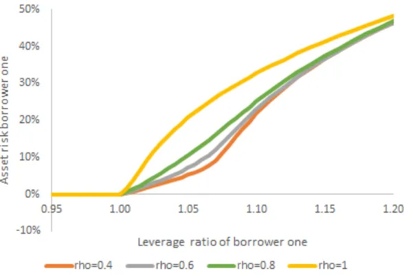
The result is relevant not only for this specific example, but also to any case where
a borrower becomes insolvent when the other borrower is insolvent. Figure 6 shows that
whenever borrower one is solvent, the level of asset risk of the insolvent borrower, borrower two, is constant. However, once borrower one becomes insolvent, where its leverage ratio is
greater than one, the level of asset risk for borrower two that maximizes equity value may
increase. This result is sensitive to the level of the correlation coefficient, as will be discussed in the next section.
The above result is consistent with “zombie lending” behavior, which is documented
empirically in Acharya, Eisert, Eufinger, and Hirsch (2016), Giannetti and Simonov (2013), and Peek and Rosengren (2005). These papers report that undercapitalized banks are found
to prefer existing low-quality borrowers to existing or new high-quality borrowers, while
well-capitalized banks do not.
7
If risk shifting had already occurred when borrower one was solvent, where the borrowers’ levels of asset risk areσ1= 10%, andσ2= 16.7%, this represents an increase of 8.6%, the values of the bank’s assets, debt,
4.3
The effect of comovements on risk shifting
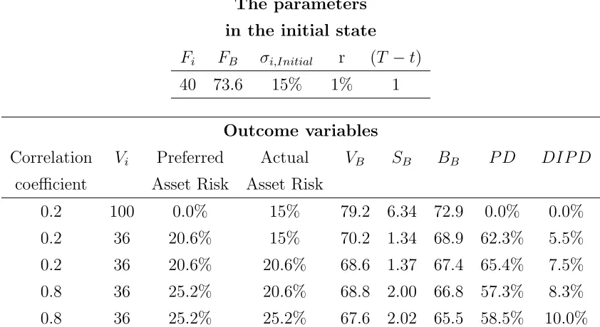
Result 3: An increase in correlation between the returns of the assets of the borrowers increases the levels of asset risk that maximize the value of the bank’s equity. Consequently, the bank’s cost of default and the value of its equity increase while the value of its assets
and debt decrease.
The financial literature shows ample evidence that in time of crisis comovements between assets’ returns increase.8 As in our paper, Gornall and Strebulaev (2018) analyze bank assets
as a portfolio of risky loans and find that, when their correlation increases, the volatility of
bank assets increases as well. Consequently, the value of the bank’s stock and its cost of default increase, while the value of its debt decreases. In this section, we show that
comovement can affect the cost of default through a second channel: its positive effect on
the stockholders’ risk-taking motivation (figure 7). Consistent with this approach, Crosignani (2017) shows that undercapitalized banks try to shift into assets that are more correlated
with their existing portfolio.
An increase in correlation between the returns of the borrowers’ assets increases the risk of the bank’s assets and therefore transfers wealth from the debtholder to the stockholder.
However, in our model, the increase in correlation not only increases the bank’s cost of default
through the increase in asset risk, but it further encourages risk shifting, since the value of the equity of the bank is maximized with a higher levels of borrowers’ asset risk. This is
because an increase in correlation increases the probability of states where the bank’s payoff
is either very high or very low, while decreasing the probability of intermediate outcomes. On the one hand, the shift between intermediate payoffs and high payoffs increases the stock
8
value, since the stock is the residual claim, while barely changing the value of the bank’s
debt, which is the senior claim. On the other hand, the shift between intermediate payoffs
and low payoff’s has a minor effect on the bank’s stock value, while greatly affecting the value of debt, i.e., the senior claim.
For example, when the value of the assets of both borrowers is 36, with a correlation of
0.2 and all other parameters are as in the base case, the level of asset risk that maximizes the
bank’s equity value is 20.6% for both borrowers. Under such conditions, the values of the bank’s assets, equity, and debt are 68.8, 1.37, and 67.4, respectively (table 3). The probability
of default is 65.4% and the value of deposit insurance per dollar of insured deposits is 7.5%.
When correlation between the returns of the two assets increases to 0.8 we find that with an asset risk of 20.6%, the bank’s asset value is virtually unchanged and remains at 68.8,
while the value of equity increases to 2.00 and the value of debt decreases to 66.8 (table 3).
The probability of default decreases to 57.3% and the value of deposit insurance per dollar of insured deposits increases to 8.3%.
We show that the increase in correlation does not affect the cost of default only in the
direct manner demonstrated above and discussed in Gornall and Strebulaev (2018). In addition, the increase in correlation increases the asset risk that maximizes the value of the
bank equity. With a correlation of 0.8, the level of asset risk that maximizes the value of
the bank equity is 25.2%. Since it is higher than the initial level of asset risk, it will also be the level of asset risk set in equilibrium. Thus, the bank’s asset value decreases to 67.6,
the equity value further increases to 2.02, and the value of debt decreases to 65.5. The
bank’s probability of default increases to 58.5% and the cost of deposit insurance per dollar of insured deposits further increases to 10.0% (table 3). These levels reflect an increase of
33% in the cost of deposit insurance per dollar of deposits, two-thirds of which is due to
risk shifting. Since risk shifting occurs when the value of the borrower’s assets is already below the face value of the debtor’s debt, the bank’s probability of default is only moderately
states of default, risk shifting substantially affects the cost of deposit insurance.
4.4
The effect of loan size
Until this section, we assume that the bank holds loans that are equal in size. This analysis is
analog to a bank with a portfolio that includes loans to two different sectors of the economy in equal weights, where the assets of borrowers within each sector are highly correlated. Such
analysis is adequate when the quality of borrowers in a major sector is deteriorating and the
goal is to study the effect on other loans. For example, the effect of the state of subprime loans during the 2007-2008 financial crisis on the equilibrium level of risk for residual loans
in a bank’s credit portfolio.
In this section, we relax this assumption and allow the size of the loans in a bank’s portfolio to differ. By studying the optimal risk level for a marginal loan we can produce
testable hypothesis for research that focuses on loan-by-loan analysis of bank risk taking.
This type of analysis is consistent with recent papers that study the effect of bank capital ratio on bank risk levels using loan-level data (Ioannidou, Ongena, and Peydr´o, 2014; Tracey,
Schnittker, and Sowerbutts, 2017; Ohlrogge, 2017).
To focus our analysis on the effect of loan size and to avoid the effect of changes in loan size on the leverage ratio of the bank’s portfolio, we analyze the case where the two borrowers
have identical leverage ratios.
Result 4: For insolvent borrowers with identical leverage ratio, as the weight of a loan in a bank’s portfolio increases, the preferred level of risk of its borrower increases as well.
The result is demonstrated in figure 8 that shows the effect of the size of a loan on the
level of asset risk that maximizes bank’s stock value. In the figure, the weight of the loan to borrower one ranges from 0% to 100%. As the size of the loan increases, the level of risk
risk of borrower one, when the leverage ratio of both borrowers is 1.1, is 23% when loans are
equally weighted and 12.3% when borrower one’s weight decreases to 25%. When borrower
one’s weight is only 1% of the portfolio, its level of risk preferred by the bank decreases to 11.5%. This example highlights the limit of diversification, although the preferred level
of asset risk is substantially lower than in the case of equally weighted loans it is still far
from being zero. At the other extreme, if we assume the bank holds only one loan whose
weight is 100% and the borrower’s leverage ratio is 1.1, the level of asset risk preferred by the bank is 32.8%. The analysis helps to understand the expected gap in the results between
a loan-by-loan analysis and an analysis that is focused on the entire risk of the bank.
4.5
Asset risk preferred by bank stockholders vs.
equilibrium
asset risk
Result 5: The equilibrium asset risk may diverge from the asset risk preferred by the bank stockholder.
Since risk shifting can occur only if both the stockholder of the bank and of the borrowers are better off, and since a borrower’s stock value always increases with its asset risk, the
optimal level of asset risk is bounded from below by the initial level of asset risk. In the case
of a bank with a single borrower, this means that the equilibrium level of asset risk is the maximum between the initial level of asset risk and the level that maximizes the value of
the bank equity (which we define as the preferred level of asset risk). In the more realistic
case of a bank with more than one borrower, the equilibrium level of asset risk may differ from both the initial and the preferred levels of asset risk, as demonstrated in figure 5.
Panel a of figure 5 presents the value of the bank equity as a function of the borrowers’
asset risk, where the leverage ratio of one of the borrowers is 0.95 and the leverage of the other is 1.1 and both borrowers’ initial level of asset risk is 10%. In this case, the risk levels
12.7% for the insolvent borrower and zero for the solvent borrower. While it is clear that the
bank’s stockholder would be better off decreasing the solvent borrower’s asset risk to zero,
this is impossible because it decreases the stock value of the solvent borrower. Therefore, the solvent borrower’s asset risk remains at 10% and the value of the bank equity is
hump-shaped with respect to the risk of the insolvent borrower and reaches its maximum when the
insolvent borrower’s asset risk is 16.8%. This equilibrium level of 16.8% is above both the
initial and preferred levels of asset risk, which equal 10% and 12.7%, respectively.
A borrower’s equilibrium level of asset risk depends in a non-trivial way on the other
borrower’s initial level of asset risk, as demonstrated in the three panels of figure 5. In panel
a, the leverage of borrower one is 0.95 while the leverage of borrower two is 1.1. The value of the bank equity decreases with the asset risk of the solvent borrower. Therefore, the
bank shareholder prevents risk shifting by the solvent borrower, irrespective of the insolvent
borrower’s level of asset risk. However, the reverse is not true: the insolvent borrower’s equilibrium level of asset risk does depend on the solvent borrower’s initial level of asset risk.
Specifically, as the solvent borrower’s initial level of risk increases, the preferred level of risk
for the insolvent borrower increases as well.
Panel c of figure 5 pertains to the case where the leverage of both borrowers is 1.1;
i.e. both borrowers are insolvent. In this case, the level of asset risk of a borrower that
maximizes the bank’s stock value is a decreasing function of the asset risk of the other borrower. The global maximum value of bank equity is 1.75 and it is achieved when the
asset risk of both borrowers equals 23%. When the borrowers’ initial asset risk is below this
5
Conclusion
To our knowledge this paper is the first to incorporate simultaneously three important aspects of bank assets. First, we assume that bank assets are composed of risky debt claims (Dermine
and Lajeri, 2001; Chen, Ju, Mazumdar, and Verma, 2006; Nagel and Purnanandam, 2015).
Second, we consider the effect of risk shifting on the equilibrium level of asset risk as well as on the bank’s cost of default (Peleg Lazar and Raviv, 2017). Finally, we assume that
bank assets are a portfolio of loans to borrowers that have different leverage and correlations
coefficients between the returns on their assets (Flannery, 1989; Gornall and Strebulaev, 2018; Nagel and Purnanandam, 2015).
We show that, in contrast to the basic agent theory, in which stockholders are motivated
to shift risk in any state (Jensen and Meckling, 1976), in our setting the bank stockholder is
motivated to shift risk only when the borrower is insolvent. Therefore, a necessary condition for risk shifting is the presence of a borrower whose asset value is below its face value of
debt. Moreover, we show that the equilibrium level of asset risk increases with a borrower’s
leverage. These results do not depend on the leverage ratio of the other borrowers and on the correlation between asset returns.
The major contribution of our work refers to the cross-borrower effects on equilibrium risk
taking. We show that if a borrower is insolvent, its equilibrium level of asset risk increases with the leverage ratio of the other borrower. Put differently, as the bank’s capital ratio
decreases, its stockholder will tolerate an increase in risk by an insolvent borrower, even
when the borrower’s leverage ratio is unchanged. This result is in line with the “zombie lending” behavior by banks (Acharya, Eisert, Eufinger, and Hirsch, 2016).
The literature presents evidence that in time of crisis comovements between the returns
of assets increases (Das, Duffie, Kapadia, and Saita, 2007; Duffie, Eckner, Horel, and Saita, 2009) and consequently the cost of default increases, while the value of debt decreases
of default through a second channel: its positive effect on the stockholders’ risk-taking
mo-tivation. When a borrower is insolvent, an increase in correlation between the returns of
its assets and the assets of the other loans increases the levels of asset risk that maximize the value of the bank’s equity. Consequently, the bank’s cost of default and the value of its
References
Acharya, V. V., T. Eisert, C. Eufinger, and C. Hirsch(2016): “Whatever it takes: The real effects of unconventional monetary policy,” working paper.
Acharya, V. V., J. A. Santos,and T. Yorulmazer(2010): “Systemic risk and deposit insurance premiums,”Federal Reserve Bank of New York Economic Policy Review, 16(1), 89–99.
Allen, F., E. Carletti, I. Goldstein, and A. Leonello (2015): “Moral hazard and government guarantees in the banking industry,” Journal of Financial Regulation, 1(1), 30–50.
Ang, A., and G. Bekaert (2002): “International asset allocation with regime shifts,”
Review of Financial Studies, 15(4), 1137–1187.
Ang, A., and J. Chen(2002): “Asymmetric correlations of equity portfolios,” Journal of
Financial Economics, 63(3), 443–494.
Anginer, D., A. Demirguc-Kunt, and M. Zhu (2014): “How does deposit insurance affect bank risk? Evidence from the recent crisis,” Journal of Banking & Finance, 48,
312–321.
Beltratti, A., and R. M. Stulz (2012): “The credit crisis around the globe: Why did some banks perform better?,”Journal of Financial Economics, 105(1), 1–17.
Brealey, R., H. E. Leland, and D. H. Pyle (1977): “Informational asymmetries, financial structure, and financial intermediation,”Journal of Finance, 32(2), 371–387.
Caprio, G., andR. Levine(2002): “Corporate governance in finance: Concepts and inter-national observations,” inFinancial sector governance: The roles of the public and private
sectors, ed. by V. S. RE Litan, M Pomerleano, pp. 17–50. Washington, DC: Brookings Institute.
Chan, Y.-S., S. I. Greenbaum, and A. V. Thakor (1992): “Is fairly priced deposit insurance possible?,” Journal of Finance, 47(1), 227–245.
Chen, A. H., N. Ju, S. C. Mazumdar, and A. Verma (2006): “Correlated default
risks and bank regulations,”Journal of Money, Credit and Banking, 38, 375–398.
Crosignani, M.(2017): “Why are banks not recapitalized during crises?,” working paper.
Das, S. R., D. Duffie, N. Kapadia, and L. Saita (2007): “Common failings: How corporate defaults are correlated,” Journal of Finance, 62(1), 93–117.
D´avila, E., and I. Goldstein (2015): “Optimal deposit insurance,” working paper.
De Servigny, A., and O. Renault (2002): “Default correlation: Empirical evidence,” working paper.
Dermine, J., and F. Lajeri (2001): “Credit risk and the deposit insurance premium: A note,”Journal of Economics and Business, 53, 497–508.
Diamond, D. W. (1984): “Financial intermediation and delegated monitoring,”Review of
Economic Studies, 51(3), 393–414.
Duffie, D., A. Eckner, G. Horel, and L. Saita (2009): “Frailty correlated default,”
Journal of Finance, 64(5), 2089–2123.
Flannery, M. J. (1989): “Capital regulation and insured banks choice of individual loan default risks,” Journal of Monetary Economics, 24(2), 235–258.
Flannery, M. J., S. H. Kwan,and M. Nimalendran(2013): “The 2007–2009 financial crisis and bank opaqueness,”Journal of Financial Intermediation, 22(1), 55–84.
Freixas, X., and J.-C. Rochet (1998): “Fair pricing of deposit insurance. Is it possible? Yes. Is it desirable? No.,”Research in Economics, 52(3), 217–232.
Galai, D., and R. W. Masulis(1976): “The option pricing model and the risk factor of stock,” Journal of Financial Economics, 3(1), 53–81.
Giannetti, M., and A. Simonov (2013): “On the real effects of bank bailouts: Micro evidence from Japan,”American Economic Journal: Macroeconomics, 5(1), 135–167.
Gornall, W., and I. A. Strebulaev(2018): “Financing as a supply chain: The capital structure of banks and borrowers,”Journal of Financial Economics, 129(3), 510–530.
Hoggarth, G., J. Reidhill, and P. Sinclair(2003): “Resolution of banking crises: An overview,” Bank of England Financial Stability Review.
Huang, J.-Z., and M. Huang (2012): “How much of the corporate-treasury yield spread is due to credit risk?,”Review of Asset Pricing Studies, 2(2), 153–202.
Ioannidou, V., S. Ongena, and J.-L. Peydr´o (2014): “Monetary policy, risk-taking, and pricing: Evidence from a quasi-natural experiment,” Review of Finance, 19(1), 95–
144.
Jensen, M. C., and W. H. Meckling(1976): “Theory of the firm: Managerial behavior, agency costs and ownership structure,”Journal of Financial Economics, 3(4), 305–360.
Longin, F., and B. Solnik(2001): “Extreme correlation of international equity markets,”
Journal of Finance, 56(2), 649–676.
Loretan, M., and W. B. English (2000): “Evaluating correlation breakdowns during periods of market volatility,” working paper Federal Reserve Board.
Marcus, A. J., and I. Shaked(1984): “The valuation of FDIC deposit insurance using option-pricing estimates,” Journal of Money, Credit and Banking, 16(4), 446–460.
Merton, R. C. (1974): “On the pricing of corporate debt: The risk structure of interest rates,”Journal of Finance, 29(2), 449–470.
(1977): “An analytic derivation of the cost of deposit insurance and loan guarantees an application of modern option pricing theory,”Journal of Banking & Finance, 1, 3–11.
Morgan, D. P. (2002): “Rating banks: Risk and uncertainty in an opaque industry,”
American Economic Review, 92(4), 874–888.
Nagel, S., and A. Purnanandam (2015): “Bank Risk Dynamics and Distance to De-fault,” working paper.
Ohlrogge, M. (2017): “Bank capital and risk taking: A loan level analysis,” working paper.
Peek, J., and E. S. Rosengren (2005): “Unnatural selection: Perverse incentives and the misallocation of credit in Japan,” American Economic Review, 95(4), 1144–1166.
Peleg Lazar, S., and A. Raviv (2017): “Bank Risk Dynamics where assets are risky debt claims,”European Financial Management, 23(1), 3–31.
Schivardi, F., E. Sette, and G. Tabellini (2017): “Credit misallocation during the European financial crisis,” working paper.
Tracey, B., C. Schnittker, and R. Sowerbutts (2017): “Bank capital and
risk-taking: Evidence from misconduct provisions,” working paper.
Appendix A: The Case of a Single Borrower
In the case of a bank with assets in the form of a risky loan to a single borrower, the value
of the bank’s equity can be replicated by a ‘bull spread’ strategy as suggested by Dermine and Lajeri (2001) (figure 2). This strategy is composed of two options. The first is a long
position in a European call option on the value of the borrowing corporation’s asset with a
strike price equal to the face value of the debt of the bank. The second option is a short position in a European call on the same underlying asset, but with a higher strike price
equal to the face value of the borrower’s debt. Thus, the value of the bank’s equity can be
expressed as
SB =Call(VC, FB, σ, T −t)−Call(VC, FC, σ, T −t), (A.21)
whereVC is the asset value of the borrower andFC is the face value of its debt to the bank.
As analyzed in Peleg Lazar and Raviv (2017), the level of asset risk that maximizes the
value of the stock of the bank can be found by taking the derivative of the value of the bank’s
stock with respect to the borrower’s asset risk:
∂SB
∂σ = √
T −t √
2π VCe −1
2σ21T ea−eb, (A.22)
where:
a=−2 lnVClnFB+ (lnFB)2−2 ln (FB)
r+σ 2
2
(T −t),
and
b=−2 lnVClnFC + (lnFC)2−2 ln (FC)
r+ σ 2
2
(T −t).
There is a constrained maximum to the value of the stock of the bank with respect to
asset risk in cases where the first derivative equals zero. There are two solutions to the
equation whenVC = 0 or when a=b. By using the terms of the equation a=b we find the
risk:
V∗∗ ≡(FBFC)
1 2e−
r+σ2
2
(T−t)
. (A.23)
Based on equation A.23, we define V∗∗ as the value of assets for which equity value is
maximized for a chosen level of asset risk σ. Note that the derivative changes its sign from positive above the threshold V∗∗ to negative below. Thus, the bank stockholder would like
to increase risk for asset values below V∗∗ and to decrease risk for values above it.
By using the same equation where a = b we can now fix the level of assets in order to find the level of asset risk that maximizes the stock value of the bank:
σmax =
s
1
T −tln
FBFC
(VC)2
−2r (A.24)
However, for both equations A.23 and A.24 to hold, that is, for an internal solution to
exist, the corporation’s asset value must be below V∗ defined as V∗ ≡(F
BFC)
1
Table 1: Risk shifting with identical borrowers and a perfect
posi-tive correlation
The base-case parameters
in the initial state
FC FB σInitial r (T −t) VC
80 73.6 15% 1% 1 74
Outcome variables
VB EB BB V∗ V∗∗ σmax σU Bound σ∗ P D DIP D
The result with initial level of asset risk
71.6 2.5 69 76 75.1 22.9% 15% 15% 48.9% 5.2%
The result with preferred level of asset risk
69.3 2.6 66.7 76 75.1 22.9% 22.9% 22.9% 51.9% 8.4%
The table presents the set of parameters and payoffs in equilibrium as well as the bank’s probability of default and cost of deposit insurance for the case in which risk shifting is impossible and for the case in which risk shifting can take place. The base-case parameters
FC,FB, σ,r, and (T−t) are the face values of the debt of the borrower and of the bank, the
borrower’s asset risk, the risk-free rate, and the time to maturity of the debt instruments.
VC, VB, EB, and BB are the sum of values of the borrowers’ assets and the bank’s assets,
equity, and debt. The thresholds for risk shifting is V∗: the level of assets below which the
position of the bank’s stockholder is hump-shaped, as defined in equation 18. V∗∗ is the threshold under which the bank stockholder is better off by increasing asset risk as defined in equation 19. The level of asset risk that maximizes the value of the bank stock, σmax
is defined in equation 20. The upper bound on the borrower’s asset risk set by the bank’s stockholder and the equilibrium asset volatility, as defined in section 3, are σU Bound and σ∗,
respectively. P D is the probability of default of the bank as defined in equation 15 and
Table 2: The effect of the borrowers’ leverage on risk taking
The parameters
in the initial state
ρ LR2 FB σ1,Initial σ2,Initial r (T −t)
0.6 1.1 73.6 10% 10% 1% 1
Outcome variables
Type of Asset Risk
LR1 Asset risk Borrower1 Borrower2 VB SB BB P D DIP D S1 S2
0.95 Initial 10% 10% 74.5 2.6 71.9 30.3% 1.4% 2.87 0.34
0.95 Preferred 0% 12.8% 75.0 2.8 72.2 28.9% 1.0% 2.08 0.64
0.95 Equilibrium 10% 16.7% 73.7 2.7 71.0 38.9% 2.5% 2.87 1.11
1.1 Initial with risk shifting 10% 16.7% 70.5 1.6 68.9 57.7% 5.4% 0.34 1.11
1.1 Initial with no risk shifting 10% 10% 71.3 1.5 69.8 57.5% 4.2% 0.34 0.34
1.1 Equilibrium 23% 23% 68.1 1.8 66.3 61.1% 9.0% 1.95 1.95
The table presents the set of parameters and the value of the bank’s liabilities and assets in equilibrium as well as the bank’s probability of default and cost of deposit insurance for the case of a bank with two borrowers. FB is the face value of the debt of the bank, r is the
risk-free rate, and (T −t) is the time to maturity of the debt instruments. The parameter
ρ is the instantaneous correlation coefficient between the returns of the borrowers’ assets.
LR1 and LR2 are the leverage ratios of the two borrowers. σ1,Initial and σ2,Initial are the
initial levels of asset risk of borrower one and two respectively. S1 and S2 are the values of the borrowers’ stock. VB, SB, and BB are the values of the bank’s assets, equity, and debt,
Table 3: The effect of correlation on risk taking
The parameters
in the initial state
Fi FB σi,Initial r (T −t)
40 73.6 15% 1% 1
Outcome variables
Correlation Vi Preferred Actual VB SB BB P D DIP D
coefficient Asset Risk Asset Risk
0.2 100 0.0% 15% 79.2 6.34 72.9 0.0% 0.0% 0.2 36 20.6% 15% 70.2 1.34 68.9 62.3% 5.5% 0.2 36 20.6% 20.6% 68.6 1.37 67.4 65.4% 7.5% 0.8 36 25.2% 20.6% 68.8 2.00 66.8 57.3% 8.3% 0.8 36 25.2% 25.2% 67.6 2.02 65.5 58.5% 10.0%
The table presents the set of parameters and payoffs in equilibrium as well as the bank’s probability of default and the cost of deposit insurance for the case of a bank with two borrowers. The two borrowers have identical capital structures and terms of loans: the face value of the debt of both borrowers is Fi and the initial asset risk of both is σi,Initial. FB
is the face value of the debt of the bank, r is the risk-free rate, and (T −t) is the time to maturity of the debt instruments. Vi is the asset value of both borrowers. VB, SB, and BB
(a) The value of a bank’s assets, debt, and equity at debt maturity.
[image:41.612.166.453.136.298.2](b) The value of a bank’s assets, debt, and equity one year before debt maturity.
Figure 3: The preferred asset risk of a borrower as a function of its leverage ratio for different correlation coefficients. The preferred asset risk for a borrower is the level of risk that maximizes the value of the bank’s equity. The figure refers to a bank with a portfolio of two loans. The figure presents the asset risk of a borrower that maximizes the value of bank equity (“preferred level of risk”) as a function of the leverage ratio of the borrower and of the correlation between the returns of their assets. The leverage ratio of the other borrower is constant and equal to LR2 = 1.1. The face value of debt of each borrower
(a) LR1 = 0.95 and LR2 = 1.1
(b) LR1 = 1.05 andLR2 = 1.1
[image:44.612.195.418.64.598.2](c) LR1 = 1.1 andLR2= 1.1
Figure 5: The value of bank stock as a function of the asset risk of its borrowers The figure refers to a bank with a portfolio of two loans. Each line represents a different level of asset risk of borrower one. The first panel depicts the case were one borrower is solvent while the other is insolvent. The second and third panels depict cases were both borrowers are insolvent. LR1andLR2 are the leverage ratios of the
Figure 6: The bank’s preferred asset risk for a borrower as a function of the other borrower’s leverage ratio. The figure refers to a bank with a portfolio of two loans. The figure presents the asset risk of borrower two which is preferred by the bank stockholder as a function of the leverage of borrower one. Each line represents a different correlation coefficient between the returns of the borrowers’ assets. The leverage ratio of borrower two is constant and equal LR2 = 1.1. The face value of debt of each borrower
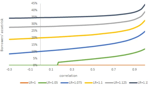
Figure 7: The preferred risk for borrowers as a function of correlation. The figure refers to a bank with a portfolio of two loans and presents the asset risk preferred by the bank’s stockholder for both borrowers as a function of the correlation between their returns. The deferent lines represent deferent leverage ratios for the borrowers ranging from LRi = 1 to LRi = 1.15. The face value of debt of each
borrower equals 40. The figure refers to the case where the bank’s face value of debt isFB = 73.6. The time
Figure 8: The preferred risk for borrower one as a function of its weight in the bank’s loan portfolio. The f