Modeling and forecasting inflation in Tanzania using ARIMA models

(1)

Munich Personal RePEc Archive

Modeling and forecasting inflation in

Tanzania using ARIMA models

NYONI, THABANI

University of Zimbabwe

19 February 2019

(2)

Modeling and Forecasting Inflation in Tanzania using ARIMA Models

Nyoni, Thabani

Department of Economics

University of Zimbabwe

Harare, Zimbabwe

Email: nyonithabani35@gmail.com

ABSTRACT

This research uses annual time series data on inflation rates in Tanzania from 1966 to 2017, to model and forecast inflation using the Box – Jenkins ARIMA technique. Diagnostic tests indicate that the T series is I (1). The study presents the ARIMA (1, 1, 2) model for predicting inflation in Tanzania. The diagnostic tests further imply that the presented optimal model is actually stable and acceptable for predicting inflation in Tanzania. The results of the study apparently show that inflation in Tanzania is likely to continue on an upwards trajectory in the next decade. The study basically encourages policy makers to make use of tight monetary and fiscal policy measures in order to control inflation in Tanzania.

Key Words: Forecasting, Inflation, Tanzania

JEL Codes: C53, E31, E37, E47

INTRODUCTION

(3)

widely recognized (Fenira, 2014). Inflation is one of the central terms in macroeconomics (Enke & Mehdiyev, 2014) as it harms the stability of the acquisition power of the national currency, affects economic growth because investment projects become riskier, distorts consuming and saving decisions, causes unequal income distribution and also results in difficulties in financial intervention (Hurtado et al, 2013). Some economists are of the view that a low and stable inflation rate of 3% has a small cost in the economy (Mankiw, 2008). In fact one digit inflation figures are not bad for growth. However, too low inflation, say below, 0%; is not healthy for any economy.

As the prediction of accurate inflation rates is a key component for setting the country’s monetary policy, it is especially important for central banks to obtain precise values (Mcnelis & Mcadam, 2004). To prevent the aforementioned undesirable outcomes of price instability, central banks require proper understanding of the future path of inflation to anchor expectations and ensure policy credibility; the key aspects of an effective monetary policy transmission mechanism (King, 2005). Inflation forecasts and projections are also often at the heart of economic policy decision-making, as is the case for monetary policy, which in most industrialized economies is mandated to maintain price stability over the medium term (Buelens, 2012). Economic agents, private and public alike; monitor closely the evolution of prices in the economy, in order to make decisions that allow them to optimize the use of their resources (Hector & Valle, 2002). Decision-makers hence need to have a view of the likely future path of inflation when taking measures that are necessary to reach their objective (Buelens, 2012).

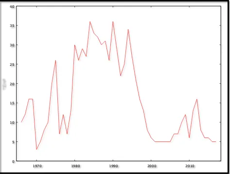
Controlling inflation within acceptable rates is one of the major macroeconomic policies in Tanzania (Laryea & Sumaila, 2001). Despite that, price stability was made a primary concern of the Bank of Tanzania (BOT), the country is experiencing volatility in inflation rates and is yet to permanently secure the target average of 0 to 5 percent annual rate (Ayubu, 2013) and figure 1 below confirms this. To avoid adjusting policy and models by not using an inflation rate prediction can result in imprecise investment and saving decisions, potentially leading to economic instability (Enke & Mehdiyev, 2014). In this study, we seek to model and forecast inflation in Tanzania using ARIMA models.

LITERATURE REVIEW

(4)

we employ annual data and rely on the Box-Jenkins ARIMA technique for estimation purposes; such an approach has not been used before, in the case of Tanzania.

MATERIALS & METHODS

Box – Jenkins ARIMA Models

One of the methods that are commonly used for forecasting time series data is the Autoregressive Integrated Moving Average (ARIMA) (Box & Jenkins, 1976; Brocwell & Davis, 2002; Chatfield, 2004; Wei, 2006; Cryer & Chan, 2008). For the purpose of forecasting inflation rate in Tanzania, ARIMA models were specified and estimated. If the sequence ∆dTt satisfies an

ARMA (p, q) process; then the sequence of Tt also satisfies the ARIMA (p, d, q) process such

that:

∆𝑑_𝑇

𝑡= ∑ 𝛽𝑖∆𝑑𝑇𝑡−𝑖+ 𝑝

𝑖=1

∑ 𝛼𝑖𝜇𝑡−𝑖 𝑞

𝑖=1

+ 𝜇𝑡… … … . … … … … . … … . [1]

which we can also re – write as:

∆𝑑_𝑇

𝑡 = ∑ 𝛽𝑖∆𝑑𝐿𝑖𝑇𝑡 𝑝

𝑖=1

+ ∑ 𝛼𝑖𝐿𝑖𝜇𝑡 𝑞

𝑖=1

+ 𝜇𝑡… … … . . … … … . … … … [2]

where ∆ is the difference operator, vector β ϵⱤp

and ɑ ϵⱤq.

The Box – Jenkins Methodology

The first step towards model selection is to difference the series in order to achieve stationarity. Once this process is over, the researcher will then examine the correlogram in order to decide on the appropriate orders of the AR and MA components. It is important to highlight the fact that this procedure (of choosing the AR and MA components) is biased towards the use of personal judgement because there are no clear – cut rules on how to decide on the appropriate AR and MA components. Therefore, experience plays a pivotal role in this regard. The next step is the estimation of the tentative model, after which diagnostic testing shall follow. Diagnostic checking is usually done by generating the set of residuals and testing whether they satisfy the characteristics of a white noise process. If not, there would be need for model re – specification and repetition of the same process; this time from the second stage. The process may go on and on until an appropriate model is identified (Nyoni, 2018).

Data Collection

This study is based on a data set of annual rates of inflation in Tanzania (TZINF or simply T) ranging over the period 1966 – 2017. All the data was taken from the World Bank.

Diagnostic Tests & Model Evaluation

Stationarity Tests: Graphical Analysis

(5)

The Correlogram in Levels

[image:5.612.78.551.75.432.2]

Autocorrelation function for TZINF ***, **, * indicate significance at the 1%, 5%, 10% levels.

Table 1

LAG ACF PACF Q-stat. [p-value]

1 0.8202 *** 0.8202 *** 37.0385 [0.000]

2 0.6911 *** 0.0561 63.8594 [0.000]

3 0.6153 *** 0.1051 85.5555 [0.000]

4 0.5413 *** -0.0004 102.6987 [0.000]

5 0.4898 *** 0.0525 117.0332 [0.000]

6 0.4527 *** 0.0388 129.5457 [0.000]

7 0.3327 ** -0.2446 * 136.4546 [0.000]

0 5 10 15 20 25 30 35 40

(6)

8 0.2123 -0.1262 139.3302 [0.000]

9 0.1306 -0.0382 140.4443 [0.000]

10 0.0732 0.0078 140.8024 [0.000]

The ADF Test in Levels

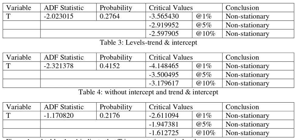
Table 2: Levels-intercept

Variable ADF Statistic Probability Critical Values Conclusion

T -2.023015 0.2764 -3.565430 @1% Non-stationary

-2.919952 @5% Non-stationary

-2.597905 @10% Non-stationary Table 3: Levels-trend & intercept

T -2.321378 0.4152 -4.148465 @1% Non-stationary

-3.179617 @10% Non-stationary Table 4: without intercept and trend & intercept

T -1.170820 0.2176 -2.611094 @1% Non-stationary

[image:6.612.62.552.186.416.2]

-1.612725 @10% Non-stationary Figure 1 and tables 1 – 4 indicate that T is non-stationary in levels.

The Correlogram (at 1st Differences)

Autocorrelation function for d_TZINF ***, **, * indicate significance at the 1%, 5%, 10% levels.

Table 5

LAG ACF PACF Q-stat. [p-value]

1 -0.1468 -0.1468 1.1643 [0.281]

2 -0.1426 -0.1677 2.2858 [0.319]

3 -0.0060 -0.0579 2.2878 [0.515]

4 -0.0973 -0.1395 2.8328 [0.586]

5 0.0109 -0.0442 2.8397 [0.725]

6 0.2420 * 0.2113 6.3584 [0.384]

(7)

8 -0.0498 0.0158 6.5848 [0.582]

9 -0.0665 -0.0613 6.8693 [0.651]

10 0.0444 0.0657 6.9993 [0.726]

ADF Test in 1st Differences

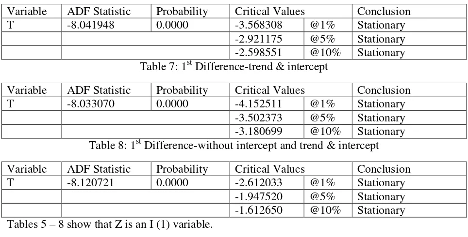
Table 6: 1st Difference-intercept

T -8.041948 0.0000 -3.568308 @1% Stationary

-2.921175 @5% Stationary

[image:7.612.65.547.187.432.2]

-2.598551 @10% Stationary Table 7: 1st Difference-trend & intercept

T -8.033070 0.0000 -4.152511 @1% Stationary

-3.180699 @10% Stationary Table 8: 1st Difference-without intercept and trend & intercept

T -8.120721 0.0000 -2.612033 @1% Stationary

-1.612650 @10% Stationary Tables 5 – 8 show that Z is an I (1) variable.

Evaluation of ARIMA models (without a constant)

Table 9

Model AIC U ME MAE RMSE MAPE

ARIMA (1, 1, 1) 331.1344 0.96461 -0.13782 4.328 5.86 40.042

ARIMA (1, 1, 0) 330.6554 0.95748 -0.11214 4.2795 5.95 38.308

ARIMA (0, 1, 1) 330.131 0.95891 -0.1241 4.2786 5.9181 38.917

ARIMA (2, 1, 1) 332.7998 0.97347 -0.142 4.3459 5.8398 39.952

ARIMA (1, 1, 2) 332.7944 0.9735 -0.14037 4.3578 5.8396 40.001

ARIMA (2, 1, 2) 334.7929 0.97306 -0.14016 4.3596 5.8396 40.021

A model with a lower AIC value is better than the one with a higher AIC value (Nyoni, 2018). Theil’s U must lie between 0 and 1, of which the closer it is to 0, the better the forecast method (Nyoni, 2018). The study will only consider the AIC as the criteria for choosing the best model for forecasting inflation in Tanzania and therefore, the ARIMA (0, 1, 1) model is carefully selected.

Residual & Stability Tests

(8)

Table 10: Levels-intercept

Rt -6.682351 0.0000 -3.568308 @1% Stationary

[image:8.612.63.550.92.330.2]

-2.598551 @10% Stationary Table 11: Levels-trend & intercept

Rt -6.702224 0.0000 -4.152511 @1% Stationary

-3.180699 @10% Stationary Table 12: without intercept and trend & intercept

Rt -6.746533 0.0000 -2.612033 @1% Stationary

Tables 10, 11 and 12 show that the residuals of the ARIMA (0, 1, 1) model are stationary and hence the ARIMA (0, 1, 1) model is suitable for forecasting inflation in Tanzania.

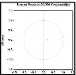
[image:8.612.172.439.399.661.2]

Stability Test of the ARIMA (0, 1, 1) Model

Figure 2

-1.5 -1.0 -0.5 0.0 0.5 1.0 1.5

M

A

r

o

ts

(9)

Since the corresponding inverse roots of the characteristic polynomial lie in the unit circle, it illustrates that the chosen ARIMA (0, 1, 1) model is stable and suitable for predicting inflation in Tanzania over the period under study.

FINDINGS

[image:9.612.71.548.186.310.2]

Descriptive Statistics

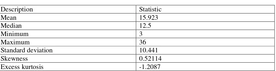
Table 13

Description Statistic

Mean 15.923

Median 12.5

Minimum 3

Maximum 36

Standard deviation 10.441

Skewness 0.52114

Excess kurtosis -1.2087

As shown above, the mean is positive, i.e. 15.923%. The minimum is 3% and the maximum is 36%. The skewness is 0.52114 and the most striking characteristic is that it is positive, indicating that the inflation series is positively skewed and non-symmetric. Excess kurtosis was found to be -1.2087; implying that the inflation series is not normally distributed.

Results Presentation1

Table 14

ARIMA (1, 1, 2) Model:

∆𝑇𝑡−1= −0.215204𝜇𝑡−1… … … . … … … . … … … . . … . [3] P: (0.116)

S. E: (0.1369)

Variable Coefficient Standard Error z p-value

MA (1) -0.215204 0.136917 -1.572 0.116

Predicted Annual Inflation in Tanzania

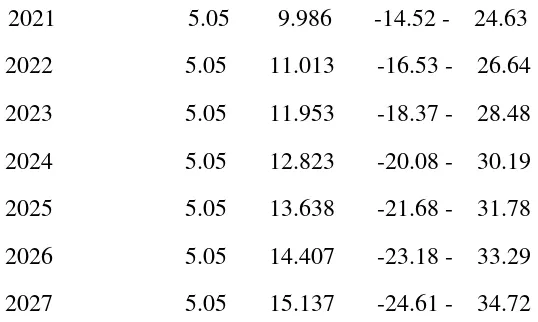
Table 15

Year Prediction Std. Error 95% Confidence Interval

2018 5.05 5.918 -6.54 - 16.65

2019 5.05 7.523 -9.69 - 19.80

2020 5.05 8.841 -12.27 - 22.38

1

(10)

2021 5.05 9.986 -14.52 - 24.63

2022 5.05 11.013 -16.53 - 26.64

2023 5.05 11.953 -18.37 - 28.48

2024 5.05 12.823 -20.08 - 30.19

2025 5.05 13.638 -21.68 - 31.78

2026 5.05 14.407 -23.18 - 33.29

2027 5.05 15.137 -24.61 - 34.72

Table 15 (with a forecast range from 2018 – 2027), clearly show that annual inflation rate in Tanzania is expected to hover around 5.05% within the next decade. However, our 95% confidence interval indicates that inflation in Tanzania is capable of shooting to as high as 34.72% per annum by 2027, ceteris paribus. Therefore, there is need for good macroeconomic policy formulation and implementation in order to maintain price stability in Tanzania.

POLICY IMPLICATION & CONCLUSION

After applying the Box-Jenkins technique, the ARIMA framework was engaged to investigate annual inflation rates in Tanzania over the study period. The study mostly planned to forecast inflation in Tanzania for the upcoming period from 2018 to 2027 and the best fitting model was selected based on how well the model captures the stochastic variation in the data. The ARIMA (1, 1, 2) model is not only stable but also the most suitable model to forecast inflation for the next ten years. In general, inflation in Tanzania; is likely to be hovering around 5.05% per annum over the forecasted period. Based on the results, policy makers in Tanzania should continue to engage proper economic and monetary policies in order to fight such increase in inflation as reflected in the forecasts. In this regard, the BOT is encouraged to rely more on contractionary monetary policy, which should be complimented by a tight fiscal policy.

REFERENCES

[1] Akinboade, A. O., Siebrits, K. F., & Niedermeier, W. E (2004). The determination of inflation in South Africa: An economic analysis, AERC Research Paper No. 143, AERC.

[2] Ayubu, V. S (2013). Monetary policy and inflation dynamics: an empirical case study of Tanzanian economy, Masters Thesis, UMEA University.

[3] Blanchard, O (2000). Macroeconomics, 2nd Edition, Prentice Hall, New York.

[4] Box, G. E. P & Jenkins, G. M (1976). Time Series Analysis: Forecasting and Control,

Holden Day, San Francisco.

[5] Brocwell, P. J & Davis, R. A (2002). Introduction to Time Series and Forecasting,

[image:10.612.172.441.70.231.2]

(11)

[6] Buelens, C (2012). Inflation modeling and the crisis: assessing the impact on the performance of different forecasting models and methods, European Commission, Economic Paper No. 451.

[7] Chatfield, C (2004). The Analysis of Time Series: An Introduction, 6th Edition, Chapman & Hall, New York.

[8] Cryer, J. D & Chan, K. S (2008). Time Series Analysis with Application in R, Springer, New York.

[9] David, F. H (2001). Modelling UK inflation: 1875 – 1991, Journal of Applied Econometrics, 16: 255 – 275.

[10] Enke, D & Mehdiyev, N (2014). A Hybrid Neuro-Fuzzy Model to Forecast Inflation, Procedia Computer Science, 36 (2014): 254 – 260.

[11] Fenira, M (2014). Democracy: a determinant factor in reducing inflation,

International Journal of Economics and Financial Issues, 4 (2): 363 – 375.

[12] Hall, R (1982). Causes and Effects, Chicago University Press, Chicago.

[13] Hector, A & Valle, S (2002). Inflation forecasts with ARIMA and Vector Autoregressive models in Guatemala, Economic Research Department, Banco de Guatemala.

[14] Hurtado, C., Luis, J., Fregoso, C & Hector, J (2013). Forecasting Mexican Inflation Using Neural Networks, International Conference on Electronics, Communications and Computing, 2013: 32 – 35.

[15] Kharimah, F., Usman, M., Elfaki, W & Elfaki, F. A. M (2015). Time Series Modelling and Forecasting of the Consumer Price Bandar Lampung, Sci. Int (Lahore)., 27 (5): 4119 – 4624.

[16] King, M (2005). Monetary Policy: Practice Ahead of Theory, Bank of England.

[17] Kock, A. B & Terasvirta, T (2013). Forecasting the Finnish Consumer Price Inflation using Artificial Network Models and Three Automated Model Section Techniques, Finnish Economic Papers, 26 (1): 13 – 24.

[18] Laryea, S. A & Sumaila, U. R (2001). Determinants of inflation in Tanzania, CMI Working Paper, CMI-Bergen.

[19] Mankiw, G (2008). Principles of Macroeconomics, 5th Edition, TSI Graphics Inc, New York.

(12)

[20] Mbongo, J. E., Mutasa, F & Msigwa, R. E (2014). The effect of money supply on inflation in Tanzania, Economics, 3 (2): 19 – 26.

[21] Mcnelis, P. D & Mcadam, P (2004). Forecasting Inflation with Think Models and Neural Networks, Working Paper Series, European Central Bank.

[22] Ngailo, E., Luvanda, E & Massawe, E. S (2014). Time Series Modelling with Application to Tanzania Inflation Data, Journal of Data Analysis and Information Processing, 2: 49 – 59.

[23] Nyoni, T & Nathaniel, S. P (2019). Modeling Rates of Inflation in Nigeria: An Application of ARMA, ARIMA and GARCH models, Munich University Library – Munich Personal RePEc Archive (MPRA), Paper No. 91351.

[24] Nyoni, T (2018). Modeling and Forecasting Inflation in Zimbabwe: a Generalized Autoregressive Conditionally Heteroskedastic (GARCH) approach, Munich University Library – Munich Personal RePEc Archive (MPRA), Paper No. 88132.

[25] Nyoni, T (2018). Modeling and Forecasting Naira / USD Exchange Rate in Nigeria: a Box – Jenkins ARIMA approach, University of Munich Library – Munich Personal RePEc Archive (MPRA), Paper No. 88622.

[26] Nyoni, T (2018). Modeling and Forecasting Inflation in Kenya: Recent Insights from ARIMA and GARCH analysis, Dimorian Review, 5 (6): 16 – 40.

[27] Nyoni, T. (2018). Box – Jenkins ARIMA Approach to Predicting net FDI inflows in Zimbabwe, Munich University Library – Munich Personal RePEc Archive (MPRA), Paper No. 87737.

[28] Pindiriri, C (2012). Monetary reforms and inflation dynamics in Zimbabwe,

International Journal of Finance and Economics, 90 (2012): 207 – 222.

[29] Webster, D (2000). Webster’s New Universal Unabridged Dictionary, Barnes & Noble, New York.

[30] Wei, W. S (2006). Time Series Analysis: Univariate and Multivariate Methods, 2nd Edition, Pearson Education Inc, Canada.