Testing Some f(R,T) Gravity Models from Energy Conditions

Testing Some f(R,T) Gravity Models from

Energy Conditions

Flavio Gimenes Alvarenga1, Mahouton Jonas Stephane Houndjo1,2, Adjimon Vincent Monwanou2, Jean Bio Chabi Orou2

1_{Department of Natural Science, Federal University of Espirito Santo, Sao Mateus, Brazil} 2_{Institute of Mathematics and Physical Sciences (IMSP), Porto-Novo, Benin}

Email: [email protected]

Received August 17, 2012; revised October 28, 2012; accepted November 18, 2012

ABSTRACT



,



f

We consider R T theory of gravity, where is the curvature scalar and T is the trace of the energy momentum tensor. Attention is attached to the special case,

R



,



2

 

f R T  R f T and two expressions are assumed for the func-

tion

 

T ,



1 1

 

2 2





n

a T b a Tnb _and

f a3ln b T3



a1 a2 b1 b2 n a3 b3 q m

 

q m _{, where , , , , , , , and are input}

parameters. We observe that by adjusting suitably these input parameters, energy conditions can be satisfied. Moreover, an analysis of the perturbations and stabilities of de Sitter solutions and power-law solutions is performed with the use of the two models. The results show that for some values of the input parameters, for which energy conditions are satis-fied, de Sitter solutions and power-law solutions may be stables.

Keywords: Modified Gravity; Energy Conditions; Cosmological Stability

1. Introduction

It is well known that General Relativity (GR) based on the Einstein-Hilbert action (without taking into account the dark energy) can not explain the acceleration of the early and late universe. Therefore, GR does not describe precisely gravity and it is quite reasonable to modify it in order to get theories that admit ination and imitate the dark energy. The first tentative in this way is substituting Ein- stein-Hilbert term by an arbitrary function of the curvature scalar R, this is the so-called f R

 

theory of gravity. This theory has been widely studied and interesting results have been found [1,2]. In the same way, other alternative theory of modified gravity has been introduced, the so-called Gauss-Bonnet gravity, f G , as a general func- tion of the Gauss-Bonnet invariant term G [3]. Other combinations of scalars are also used as the generalised



,



f R G and f R P Q



, ,



[4,5], where P R R _  and

Q R _R (here R_ and R_ are the Ricci ten-sor the Riemann tenten-sor, respectively).

In this present paper, attention is attached to a type of the so-called

is performed. Also in the same way for exploring cosmo- logical scenarios based on this theory, f R T



,



CDM

func- tion has been numerically reproduced according to holo- graphic dark energy [8]. Moreover it is shown that dust

reproduces  , phantom-non-phantom and the

phantom cosmology with f R T



,



CDM

theory [9]. The gen- eral technique for performing this reproduction of

 model in FRW’s metric cosmological evolution

is widely developed in [4,10]. The f R T



,



models that are able to reproduce the fourth known types of future finite-time singularities have been investigated [11].

Note that singularities appear when energy conditions are violated. Our task in this paper is to check the viabil- ity of some models of f R T



,



according to the energy conditions. The energy conditions are formulated by the use of the Raychaudhuri equation for expansion and is based on the attractive character of the gravity. We refer the readers to Refs. [12-17], where energy conditions are widely analyzed for the cosmology settings, in f R

 

and f G

 

gravities.



,



f

In this paper, we assume a special form of R T ,

that is,



,



f R T

 

theory of gravity, where T

denotes the trace of the energy momentum tensor. This generalization of



,



2

 

f R T  R f T

T

 

, the usual Einstein-Hilbert

term plus a dependent function f T . Two expres-

f R



gravity has been made first by Harko et al. [6]. In [7], the cosmological reconstruction of f R T



, describing transition from matter domi- nated phase to the late accelerated epoch of the universe

sions of f T

 

, 1 1

2 2

n

n

a T b a T b



and are

in- 3ln



3



q m

a b T

In order to reach the acceptable cosmological models, w

this work.

In Section 2, we br

1 2

e analyse the perturbations and stabilities of de Sitter solutions and power-laws solutions in the framework of the special R2f T

 

gravity, by using the two models

proposed in We observe that for some values

of the input parameters, for both models, the stabilities of de Sitter solutions and power-law solutions are realized and compatibles with some energy conditions and the late time acceleration of the universe.

The paper is outlined as follows.

iefly present the general formalism of the theory, put- ting out the general equations of motion for a



,



 

 

f R T  f R  f T gravity, where f R1

 

and

 

2

f T and a

scalar a

re respectively function of the curvature nd the trace of the energy momentum tensor. The Section 3 is devoted to the general aspects of the energy conditions. The f R T



,



 R 2f T

 

gravity is as-

sumed in the Sectio ctions considered

for

 

n 4, where the two fun

f T are studied, putting out the conditions on the

inpu meters for obtaining some viable models of



,



t para

f R T . The perturbations and stabilities of de Sitter and solutions are investigated in the Sections 5. Dis-cussions and perspectives are presented in the Section 6. power-law

2. General Formalism

gravity replacing the Ricci Let us assume the modified

scalar R in Einstein gravity by an arbitrary function



,



f R T , and writing the total action as





d ,

2

S x g f R T



 1 4  _  _

 



L , (1)

8πG

  , Gbeing the gravitational constant and

T

where

T g  the nso whic

 trace of the matter energy momentum

h is defined by

te r





2 g

T_  

g g

 

 L

(2)

This modified gravity theory has been considered first in [6] and the equations of motion, using the metric for-malism, have been explicitly obtained as

 





1 1

2 2

1

2

2

1 2 1

R R

T T

f R f R g g f

T f T f p f g

    

  

   

 

  _  _

 



(3)

3. Energy Conditions

ssentially based on the Ray- The energy conditions are e

chaudhuri equation that describes the behaviour of a congruence of timelike, spacelike or lightlike curves. For the purposes of this work we will just consider the time- like and space-like curves for which the Raychaudhuri

equation reads, respectively [18,19]

2 ₃

R V V          d d  0 (4)

2 _{2 d d 0}

R k k          

where

(5)  is the expansion scalar describing the e v

xpan- sion of olume, and  are positive parameters used to describe the curved o the congruence, f _the shear tensor which measures the distortion of the vo me, lu _ the vorticity tensor which measures the rotation of curves, and V

the

 _{and k} _{are respectively timelike and}

lightlike vectors tangen to the curves. In this work, we are interested to the situation for small distortions of the volume, without rotation, in such a way that the quadratic terms in the Raychaudhuri equation may be disregarded (they are like second order corrections). Then, the equa- tion can be integrated given the scalar of expansion as a function of the Ricci tensor:

R V V

t

R k k

 

     

   (6)

The condition for attractive gravity is  0, impos- ing R V V   and R k k  . These two tions are

calle ng and rgy conditions, respectively.

For equivalence to GR, by just dividing by condi

d the stro null ene

 

1

f R

(different from zero), one can cast Equation (3) in the following form

1 2

eff

R_  Rg_ T_ (7)

where the effective energy momentum tensor Teff

 is

defined by













2 1

1

2 2 1 1 1

1

1 ₂

2

T R

R

T R

R

T T f T g f

f

f p f f Rf g

f

     



    

   



(8)

Thus, the null energy condition for the effective per- fe

0 eff peff eff

ct fluid reduces to

   . (9) For the strong energy conditions, one has

0, eff peff

    eff 3peff 0

.

(10) The weak energy condition for the e

flu

0 eff

ffective perfect id reads

  ,



eff peff



0, (11)

and the the dominant energy condition results in 0

eff

  ,  eff peff 0,  eff peff 0. (12)

Therefore, the nergy conditio , as known in al

e ns GR, can

In what follows, we will consider models of type



,



2

 

f R T  R f T , i.e., the usual Einstein-Hilbert ing term 2

 

term plus trace depend f T . This amounts to

consider f R1

 

R and f T2

 

2f T

 

. The factor 2

is used ju more easier to

be treated. We will also assume that the ordinary content of the universe is pressureless and satisfies the energy conditions (just eff 0

 st for letting the field equations

  ).

4. Testing Some

f R T



,



nergy Co

 

 R 2f T

nditions

In

Models from E

this section we will present the conditions required on  and the algebraic function f T

 

for realizing each pe of energy conditions. For t nd, we first need to establish the respective expression of the effective energy density eff

ty his e

 and effective pressure peff . According to the assum ons made at the end of the previous section, Equation (7) becomes

pti

1 ₂

2 T

R_ Rg_ T_  f T_ fg_. (13)

Considering the at FRW space-time described by the m

 

2_ 2_{a t dx}2 2 ₍₁₄₎

where a(t) is the scale factor. The

eff etric

ds dt

00 and ii components of (22) can be written as

2

3H  , (15)

2

2H 3H p_eff

  , (16)

where the effective energy density 



and pressure are de-fined as

 

 

T 2

eff f T  f T , (17) eff

p f T . e above expr

de

  

 

  (18)

By using th essions of the effective energy

nsity and pressure, we get the null energy condition (NEC), the weak energy condition (WEC), the strong energy condition (SEC) and the dominant energy condi- tion (DEC) by

NEC:  eff peff  1 2fT

 

T 0; (19)

WEC: eff   2fT  f 0,  eff peff 0

0,

T 

(21)

2 0,

0 T

p  f f 

 (22)

positive and non-null. This is

4.1. Studing the Case

 

; (20)

 1 1

2 2

n

n

a T b f T

a T b  

ut the constraints on the input parameters in order to get a R2f T

 

type model that

ing that a

SEC : 3p 2f 2f

0; eff eff

eff peff

  

DEC :_eff  _eff   2 0, eff peff eff

   

and b3 is assumed to be

form chosen due to its interesting aspect, in curing the big rip [11].

Our task here is to put o

satisfies the energy conditions. According to the sign of

the parameter n, and assum 2 and b2cannot

be identically null, the model can be cast into two differ- ent forms. In fact, for the late time stage of the universe, by dividing the parameters of the model by a n2



0



and b n2



0



, one gets respectively the models

 

1

2

n _B

f  _n

B



 

and

 

 

1

2 1

n

n

A f

A

 

   

 , where the

cosmological constant is characterized by a1 _(for

0

n ), and

2 a

1

b _{(for n 0}

2

b  ), and

1 a A₁ ,

2 b

2 a A₂ ,

2 b

1 b _and 1

2 B

a

 _{B }b2 _{. I is case, de h}

ameters dependent, under the cos-

2 2

a n th the mo l whic

initially was four par

mological constraints, becomes three parameters de- pendent, ,B₁ and B₂ for n0, and , A₁ and

2

A for n0. Since the cosmological constant is known

[14], the m de urns in two pa ters dep .

The f erivative of

o l t to rame endent

irst d f T

 

with respect to T (or

the derivative of f

 

 with respect to ) reads

 





₁





2

1 2 ,

n n

f_  n B    B n

 









2

2 1

1 2 2

, 0

1 , 0

n n

B

f  n A A   A n

    

     23)

4.1.1. The NEC

Since we have assumed that the ordinary content of the all the energy conditions, the condition

(

universe satisfies

(19) reduces to 1 2 f TT

 

0, (or 1 2 f

 

 0).

One can calculate 1 2 f_

 

 0 as













2 1

2 1 2 2 2

, 0,

2 n

B B

B 



 _{  }

2 1 2

n n

n B

f      n

 (24)













2 1

1 2 2 2 2

2 1

1 2 , 0,

2 1

n n

n

n A A A

f n

A 

 



 _{   }

  

 (25)

whose the sign can just be characterized by that of numerator, since the denominator is always positive. If

the

* B10, B20, B B1 2  for n0,

* A10, A20, B B1 2  for n0,

r n0, 0

 0 r n0.

d, t e tions d to the positivity

and

2 0 for n0.

Observe that there are still situations in hich the

above quantities are negative but merators in (25)

co

* 1 , ,fo

A

0

 B 0

B 2

A 

* 1 , ,fo

ee abov2

Ind he condi lea





1

2 1

2_nn _{ B B }0_{for n0}



1 A2



1

n

n  A

w the nu ntinuing positive, i.e.,

* A₁A₂ and 1









2

1 2 2

2_nn _{A   A A}n _1 for n0,

* B₂B₁ and _n





_



_n_B2



2

0

n

these case plot the function in terms o

of the parameters, fixing the other. Despite knowing th

This condition is realized when the NEC is, plus the con-

1

2 1

2n   B B

for .

In s, one can f

two

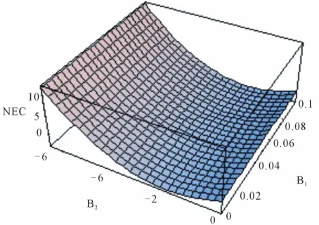
e sign of the considered parameters with what respect the function may be plotted, the important here is their rank, i.e. the interval to which they must belong in order to produce the positivity of the function. Some examples are presented in Figure 1.

4.1.2. The WEC

dition  _eff 0. Note that the complete expression and

2 1

2 n _{ } 0,_n0

These expressions are obtained by multiplyin

numerators (25) by

condition of the NEC read





1 1 2

2 1

2_{n  B B }n_n _2_{B }n _{B }0,_n0_{, (26)}

2





2 1

1 2 2 2

2_{n A  A }n_{A }n _{ A}  _{. (27)}

g the

in  . We didn’t need to us

co

[image:4.595.58.285.542.702.2]

e this mplete expression for determining the conditions on the input parameters in the case of the NEC, since the

Figure 1. The graph representing the NEC in functions of

1

B 1 , 1.7.

Be to nd (27 the second co ition for

satis-ordinary energy density is assumed as positive quantity.

sides (26) a ), nd

and B₂with 0.1

fying the WEC is

2 0

eff f f

      , (28) having in mind that the ordinary con

pressure-less. By using

tent is assumed as

 

f  , acco

1

2 1 2 1 0,

n

B B



  (29)





2 2 2 1 1 1 2 2 2

1 2 1 2

2

2 2 0, 0

n n n

n

A A A A

nA nA A A n

   



 

    

rding to the func- tions in (23), (28) becomes





2 2 1 2

2 2 1 2

2

2 2

n n _{B B B B}

n B nB

   

    

    

        (30)

Note here that we just use the numerator of

tions whose the denominators are always positives. By co

2 1

1 4n B 1 4n B  0,n 0

the frac-

mbining (26) with (29) and (30), one gets for the WEC









2 2 1 1 2

2 2 1 2

2 4 2

n n n

n

B B B B

     

    

_     _  









2 2 1 1

1 2 2

1 2

2 4 2

1 4 1 4 0, 0

n n n

n

A A A

n A n A n

   



 

    

(31)

_    _   (32)

We address here the evident conditions fo WEC is satisfied as follows:

r which the

* B10, B2 0 for 0 n 1 4,

* A10, A20, for 1 4 n 0.

s obvious that th ditions are ot unique. For n >

0 ( the necessit otting the fu tion



1 4n



B2



1 4n B



1  B B1 2

_     _  (33)









2 2 2 1 1

1 2 2 2

1 2

2 4 2

1 4 1 4

n n n

n

A A A A

n A n A

It i ese con n

n < 0), y of pl nc

2 2 1 1 2

2 2

2 4 2

n n n

n

B B

     

   

  



 

  



_    _   (34)

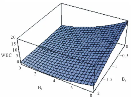
varying two of the input parameters. examples of these cases in Figure 2.

The strong energy condition is realized by combining the

3p 0

We present some

4.1.3. The SEC

NEC with eff  eff  . This latter reads,

f 3 eff 2 2 0

ef p f f

       . (35)

Making use of the expressions in (23) fraction whose the denominator is always th

, one obtains a positive and e numerator reads









2 1 1 2 2 2 2

2 2 1 1

n n n

n

B B n B2 n B1

1 2

2 2B B 0 for n 0,

  _   _ _{      }

 



     (36)









2 2 1 1

2 2 1 2

2 1 2

2 2 1 1

2 2 0 for 0,

n n n

n

A A n A n A

A A n

  



 _  _{     }

 _ _

     (37)

[image:5.595.58.286.83.252.2]

Figure 2. The graph of WEC in terms of suitable values of

1

B 1.7 , 0.1

Figure 3. The graph of the SEC in functions of B1and B2, setting

and B2with n1 ,   .

the following conditions for the SEC

2_{ B B}

1

2 2 2

, 0

n

n

A

n

 



  _{  }

  .

In this case, there is any obvious condition for satisfy- ing the SEC. However, values can be found,

the corresponding functions in terms of two of the pa- ra

is characterized by the

WEC com eff peff 0

Now, combining (36) and (37) with the NEC, on gets

1.7 , 0.1









2 2 1 2

2 1

2 2 4 2 2

2 1 2_{n B} 1 2_{n B }n 0, _n 0

 _     _   (38)

2n 1 2n _B n 1 _B

  _{ } _   _









2 2 1 2 2 1 2

1 2

2 2 4

2 1 2 1 2

n n

A A A

n A n A

   

 _    _ (39)

by plotting

meters. Some examples for illustrating some of these cases are presented in Figure 3.

4.1.4. The DEC

The dominant energy condition

bined with    . Following the

ious cases, one easily obtains the

2



1 2

0, 0

n

n _n

 

   

 

0

 , B

same steps as in the prev DEC as









2 1 2

2 2 1 2

2 2

2 1 1 2 0, 0

n n

n

B B B B

n B n B n

   



 _{  }  _{ }

_        (40)

1

2 1

n









2 2 1 2 2 1 2

1 2

2 2

2 1 1 2

n n

A A A A

n A n A

  _  _ 

_    _

The evident conditions read

(41)

1

B ₂0 and

1 2

n . Evidently, ay lead

complishment of the otting the func-

tio me of ese case

Figure

il e fundamental conditions for

which the model allows the avoidance of the Big Rip. So, other conditions

DEC, bu m t, only pl

to the ac-

ns in (40) and (41). We present so th s in

4.

4.2. Studying the Case a₃lnq



b T₃ m



Here we w l work with th



[image:5.595.310.535.85.252.2]

  and n1.

Figure 4. The graph representing the DEC in functions of

1

B and B₂with 0.1, n1, 1.7.

h la

t g th rst derivative

we propose to check if the range of parameters for which t e singu rity may be cured can also make the model

isfyin e energy conditions. Here, the fi sa

of f

 

 also plays an important role. Deriving f

 

 with respect to the energy density  , one gets

 

3 1





3

lnq m

qma

f   _  b (42)

We believe that each step of constructing the four en-ergy conditions is now clear and we si

results and comments as follows:



3 0

mply present the

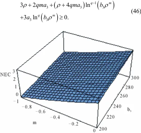
4.2.1. The NEC



1 3

2_qma lnq _b m

_{ }  _{ . (43)}

nditions for obtaining this are q0, The evident co

0

m ,a30, with 1 3

m _b

  . It is important to note

[image:5.595.311.535.285.470.2]

di

realized. This situation require





1 3

lnq _b m

fferent from the above ones, the NEC could still be s knowing some intervals to which the parameters must belong. We present this feature by plotting the function corresponding to the ex-pression (43) in terms of some of the input parameters fixing the other. See Figure 5.

4.2.2. The WEC







lnq

a b



3 3

3 3

2 2 2

0, m

qma qma

  



  





(44)

In this case by plotting the function (44), th be realized graphically. This is the set of situations one of the terms in the sum (44) is negative, but it abso- lu





1 3

lnq _b m



[image:6.595.310.537.82.243.2]

e WEC can where

Figure 6. The graph of the WEC in functions of m and b

te value is less that the absolute value of the sum of the other. See Figure 6.

4.2.3. The SEC





2 2qma3 3

3

2

) 0 m

qma

3

2 ln (_a q _b

  

  



(45)

In this case, evident constraints on the in ters in order to realize this energy conditio

 0 , a 0 , with

 



put parame- ns are pre-

sented as follows: q 0 , m 3

3

1

m _{ b . As presented in the previous cases, other}

conditions may also realize this energy conditions. This

can be observed by plo he function n terms

nput parameters, fixing the other. See Figure 7.

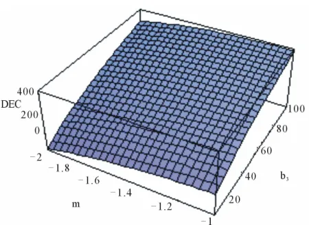
4.2.4. The DEC



tting t in (45) i

of some i





1





3

lnq _b m





3

3 ln_a q

3 3

3

3 2 4

0. m

qma qma

b

   

(46) 

  

 

Figure 5. The graph representative of the NEC in terms of m and b3, with 0.1, a3

3

using

,

0.1

[image:6.595.313.536.273.450.2]

 , a₃1 and q3.

Figure 7. The graph of the SEC in functions of m and b , 3

sing ,

u 0.1 a₃10 q 3.

Here, constraints may also lead to the DEC, but this is clear by plotting the function (46), as in the previous cases. We present an illustrative example in

Figure 8.

We mention that for all the graphs, the parameters are normalized to ₁₀121 _{Planck units. Remark that the cur-}

rent value of the cosmological constant is about

121

1.7 10  and the energy density of the usual matter is about _{0.1 10} 121 _{[14]. Then, with the normalization,}

we get 1.7

3

and 

 and 0.1

 for the cosmological con-

stant and the energy density of the usual matter respect- tively, which are the values used for plotting the graph in the figures.

)

avity

n

5. Perturbations and Stabilities in R + 2f(T

Gr

I this section we propose to study the perturbations around the models used in this work. We can start estab- lishing the perturbed equations for the case R2f T

 

, [image:6.595.59.287.485.699.2]

[image:7.595.59.284.80.244.2]

Figure 8. The graph of the WEC in functions of m and b3,

with 0.1, a₃1and q3.

but the two models will be studied as specific cases. For this purpose, let us assume a general solution for the cosmological background of FRW metric, which is given by a Hubble parameter H H t_b

 

that satisfies the background Equation (17) sing (15), fou r R2f T

 

gravity. The evol y density can

be expressed in pa tion by

solv-ing the continuity ou

ution of the terms of this

equation ar

matter energ rticular solu nd H t_b

 

,

 

3 0

b t H tb b

    , (47)

yielding

 

3 d

0e b

d d

 

H t t

 _  _{. (48)}

We recall that we are considering that the ordinar

sting in e perturbations around the solu-

 

b b t

y content of the universe is pressure-less. Since we are

intere studying th

tions H H t , we will consider small deviations

i.e.,

 

t 1

from the Hubble parameter and the energy density, we can write the Hubble parameter and the ordinary en- ergy density as [20]

 

_b

 

1

  

, _{b m}



H t H t   t   . (49)

In order to study the behavior of these perturbations in the linear regime, we expand the function

 

 

f T in powers of T_b (or _b ) evaluated at the solution

 

b

H H t , as

 

 

b b





2

b

f T  f   f  f_   O , (50)

where the superscript b refers to th

of

 

e background values

f T and its derivatives evaluated at T Tb (or b

  ). Here, the O term includes all the terms propor- tional to the square or higher powers of T (or  ). Then, only the linear terms of the induced perturbations

will be o . Hence, by making use of the expres-

sion (50) in the Equations (15) and (17), one gets the equation for the perturbation δ(t) in the linear approxi- mation,

c nsidered





 

 

2 2

6 .

b b

b b m

b

3 2

b f f t

H t

 

  

 



 

(51)

On the other hand, there is a second perturbed equa- tion from the matter continuity equation,

   

3 0

m H tb t

    _{. (52)}

By combining Equations (51) and (52) one gets the following equation for the matter perturbation



2



2 3 b 2 b 0

b m b b b m

H     f_   f_   , (53)

from which we obtain





1 _d 2 1e ,

1 3 2

b

C t m

b b

b

b b

C

C f f

b

H  



 _

 _



   , (54)

where C1is an integration constant. By using

(52), the perturbation δ reads

the relation

 

C C 1_C td

Let us now consider two cosmological solutions and analyze their stability by the use of t

this work:

In de Sitter solutions, the Hubble parameter

1 _e 2

6

b

b

b

t

H

   . (55)

he models treated in de Sitter solutions and power law solutions.

5.1. Stability of de Sitter Solutions

is constant and one has

 

 

0

0, 0e

H t b

H t H a t a , (56)

where H0 is constant.

With this scale factor, the energy density

ground becomes 3 0

0e

of the back- H t

b

 _  _{, with which one has}

0

db 3H bdt. By using this, one can cast the integral in (55) into





2 0

1

d 1 3 2

3

b b

b b

C t f

H   f db. (57)

   





5.1.1. Treating the Model

 





1

 

2



n n

f T T B T B

This case corresponds to n > 0, and the integral (55) can be expressed as









0

2 1 2 1

2 2

0 2 ₂

3 0

,

e

b

b n _n

b _b

nH t

n n

B



 _

  

2 1

d 3

n

b

n B B

B B

C t

H B



b

 _{   } 

 _{ } 

 

  _ 

 



(58)

an











2



2 1

2 1 n

b

b b

n n B B









0 ₂ 2 2 2 1 3 2 1 4 . n b n b n b C H _B

n B B

B    _{  }        _     _    _ (59)

om (58) and at for n0, and as the

time evolves, the stability of de Sitter solutions requires

les 0and b2 0

We see fr (59) th

d onl

2 0

B  . In other word, for the initial model, de Sitter

solutions are stab if an y if a2  .

5.1.2. Testing the Model



 



 

1 1 1

n n

A T

 

0

n f T  A T 

This case corresponds to  , and the integral (57),

tiplied by

mul 1 2, can be expressed as













0

1 2

0 2 2

3 0 1 2 2 2 2 2 2 1 ,

6 1 ₁

e b n b b _n n b _b nH t n n b

n A A

A A

H A A _A

   _     _{   }        _{ }   (60)

and Cb is written as 1 d C t 



 



















1 2 2 0 ₂ 2 1 1 1 n b

b b _n

b

n n A A

C H _A 2 2 1 2 3 2 4 . 1 n b n b

n A A A

A 2     _{  }     _  (61      _   ) e

. T ill grow expo-

nentially, and this particular de Sitter solution becomes ble. Note that this result does not depend on any of

1





Here, for n0, as the tim evolves, both (60) and (61) tend to  hus the perturbation w

unsta

the parameters A or A2.

5.1.3. Treati 3ln



3



q m

a b T

With this m (57), m ltiplied by

ng the Model

odel, the integral u 1 2,

can be performed and one gets





3 3

0





1

3 3

2 1

ln 2 ln

6 b

q m q m

b a b mqa b

H   



 

 _   _ (62)

with the corresponding e ession of Cbbeing 1 d C t 



xpr





1 3 3 0 1 ln 2 q m b b

C qma b

H m      _   (63) all





2





3 3

1 lnq m .

q q_ a  b _



Let us rec that this model 3ln



3



q m

a b T , leads to

the avoidance of the Big Rip for q2 



1



and 0

m , where  1, as we have previously shown.

These condition also a ws llo the model to satisfy the en- ergy conditions. Now, let us check what happens about nditions. First, note that the the stability with these co

relation q2 



1



can be cast into





2 2 1

q   , showing that q2 becau f

1

se o   . By choosing a30, we see that, within the con- ditions q2 and m0, the expressions (62) and (63) tend to  as the time evolves, and this ensures the de cay of the perturbation, leading to the stability of ter solutions with this model. Thus, regarding to the sta- bility of de Sitter solutions, the energy conditions and the

ith onditions

3 0 a

- de Sit-

late time acceleration, provided w the c

 , b30,q2 and m0, we can conclude that

the model may be cosmologically acceptable.

5.2. Stability of Powerlaw Solutions

As we are dealing with dust as ordinary content of the universe, we will be interested to the scale factor

 

2 3

 

0 2

0 2 , 3 b b a

a t a t H t t

t 



    . (64)

5.2.1. Treating the Model



 



 

 n n

1 2

f T 

In this case,

T B T B

0

n ,andone can perform the integral

  























2 2 1 2

0 2 2

2 2

2 1 2 1

2 2

2

2 2

2

2 1 2

3 4

1 3 _ln

2 4 1

4 7

2

2 1

1 1

,1,1 ; ,

n

n

n

n B B t

C t

a B B t

B B t n B B t

B B n B t

F B t

n n  _{  }                     _   _  



(65) d b t with



















2 2 1 2 2 2 1 3 1 2 n b _n

n n B B t

C

a t _{t B}

   _{  }     _ 0 ₂ 2 4 2 1 3 2

4_{n B B t} n

B      _    _ ve set 2n t

, (66)

where we ha  0 1, and 2 1F is the hypergeom

ric function d d by

et-efine





   

1

 

2 2 1 1 2 3

0 3 , , ; ! r r r r z F z r r        





, (67)

with

As the time evolves, conditions are required for guar-anteeing the decay of the perturbation. For B20, it is

necessa have B B that B1 can

be po eg

ry to

sitive, or n ative but with2 1

, which means

2 1

B B

  . In the case

her erve two sub-cases,

an eve and an r an even r, as the time

evol n for guaranteeing the

decay B2 b1

w e B20

n r,

ves, the necessa of the

one may obs odd r. Fo

ry conditio perturbation is

i.e., for

  , meaning that the

param positive. On the other

ent for getting the decay

th B10.

5.2.2. Treating the Model





eter B1 can

r an od e perturbat

d r

ion i

be negative, or , the requirem

s B2B1

hand, fo

of , meaning that

 







f T A T  

Here, n0, and the inte1 2

n n

A T  

gral can be performed as

  













2

1 2

2

1 2

2 2 2

2 2

2 2 1

2

2 3

1 3

d ln

2 4 2

3 )

2

( )

1 1

,1,1 ; ,

b _n

n

n

n A A t

C t t

a A t

A A t

t

A A t

t F

n n A

 _{  }



   

 



  





 _

 _   _

 _



, (69)

with

0 2

2 2

1

(

n A  A





















2 1

1 2

2 2

0 ₂

2 4 1

2 1 2

3 2 2

2 1

3

2 ₁

4

. 1

n

b

n

n

n

n n A A t

C

a _{A t}

A n A t

A t

 



 



 _{  }

 

 _





  _





 _

(70)

As the time evolves, the argument of the hyper-geometric function tends to zero and the hyperhyper-geometric

function tends to 1. Th e dominant ter

A

us, th m in (77)

reads







2

3

2 1 2

2 0 2

4a A A n A  A t . (71)

Here, one can distinguish two cases: (A₂ n 0 and

1 2

A  A ) and (A₂ n 0and A₁ A₂). In the first

2

  case, one gets A n m

th

eaning that A2 can be positive, i

or negative but w A2  n . When A20, A1 can be

gative, due on 1 2

positive or ne to the relati A  A , while

for A20, A1 is n tive. In the second

2

ecessarily nega

case, one gets A n, meaning that A₂0, which allows A₁ to be positive, due to the relation A₁ A₂.

e that som s for which the

ty occurs, are also compatible with some energy ns. This shows that for some values of the input parameters, acceptable models can be obtained, at least regarding to the energy conditions, the stability, the late

time acceleration of the universe and the avoidance of the Big Rip.

5.2.3. Treating the Model 3ln



3



q m

a b T .

As we have done in the previous cases, the integral can be performed, yielding

We observ e of the condition

stabili conditio

 

 





 

 





1

3 3

2 3

1 1, ,

ln m ,

3 3 0

1

1 _d 3 _ln 1 _,

2 4 2

q m b

q m

g t

C t t a qb m q

a m

g t

  

      

  





 



a q q m b q

m

g t b t

    



 



(72)

with











1

3 3

2 2

3 3

3 1

ln 2

2 1 ln

q m

b

q m

a

a q q m t b







 _ 



 

(73)

A previously mentioned, this model cures

the Big Rip for and m0. With e condi-

tions, a he time evolves, only the term



2 0

2 _.

C a qmt b t

t

t 





 s we have

2

q thes

s t ln

 

t grow s.

Since 3ln

 

t

 

4a₀ is negative for large value of the time, it is easy to observe that the perturbation decays, and this corresponds to the stability of the power law solutions with this model. Observe that in this case, the constraints on the parameters q and m for which all the energy conditions are satisfied, leads to the stability of the power-law solutions. Thus, regarding to the stabil- ity, the energy conditions, the late time acceleration of

nce of the B n

the universe and the avoida ig Rip, we ca

conclude that this model can be cosmologically accept- able for a30, b30, q2 and m0.

6. Discussions

We studied the viability of two f



R T,



models ac- cording to energy conditions. A special attention is at- tached to the models of type R2f T

 

. For t models of

he two

 

f T considered, it is shown that for some values of the input parameters, energy conditions are satisfied. Moreover, we showed that there exist values of

puts parameters for which the four energy condi- tions may be satisfied simultaneously, for the two mod- els.

An interesting feature of these models is tha

well with the observations data. Therefore, the graph re

.

nalys of the model

the in

t there fill

presenting each energy conditions in plotted for both models under study

Moreover, in order to make a consistent a is of the

stability s, we studied the stability of de

d

7. Acknowledgements

hanks Prof. S. D. Odintsov for useful for finan

ry much t estion

S. Nojiri and S. D. Odintsov, “Introduction to Modified

However, for the power-law solutions, the stability can be observed for each model un er some conditions. We also see that for the conditions for which the stability is realized, the late-time cosmic acceleration and the avoidance of the big rip are always satisfied. We con- clude that, in the frame work of R2f T

 

gravity the two models can be viable.

M. J. S. Houndjo t

suggestions and also CNPq/FAPES cial support.

A. V. Monwanou thanks IMSP-UAC for financial

sup-port. The authors also thank ve he referees for

useful sugg s for the reorganization of the

manu-script.

REFERENCES

[1]

Gravity and Gravitational Alternative for Dark Energy,”

International Journal Geometrical Method Modern Phy- sics, Vol. 4,No. 1, 2007, p. 115.

doi:10.1142/S0219887807001928

[2] S. Nojiri and S. D. Odintsov, arXiv: 0801.4843 [astro-ph]. arXiv: 0807.0685 [hep-th].

[3] S. Nojiri, S. D. Odintsov and P. V. Tretyakov, “From In- flation to Dark Energy in the Non-Minimal Modified Gravity,” Progress of Theoritical Physics Supplement, No. 172, 2008, pp. 81-89. doi:10.1143/PTPS.172.81

[4] A. de la Cruz-Dombriz and D. Seaz-Gomez.

[5] S. Nojiri and S. D. Odintsov, “Modified Gauss-Bonnet Theory as Gravitational Alternative for Dark Energy,”

Physical Letter B, Vol. 613, No. 1-2, 2005, pp. 1-6. doi:10.1016/j.physletb.2005.10.010

[6] T. Harko, F. S. Lobo, S. Nojiri a intsov, “f(R,T) Gravity,” Physical Review D

nd S. D. Od

, Vol. 84, No. 2, 2011, Arti-cle ID: 024020. doi:10.1103/PhysRevD.84.024020

struction of f(R,T) Gravity

41 [8] M. J. S. Houndjo and O. F. Piattella, “Reconstructing f(R,

T) Gravity from Holographic Dark Energy,” International Journal of Modern Physics D, Vol. 21, No. 3, 2012, Arti-cle ID: 1250024. doi:10.1142/S02182718125002

akulov, “Re- [9] M. Jamil, D. Momeni, M. Reza and R. Myrz

construction of Some Cosmological Models in f(R,T) Gravity,” European Physics Journal C, Vol. 72, 2012, p. 1999. doi:10.1140/epjc/s10052-012-1999-9

[10] S. Nojiri, S. D. Odintsov and D. Saez-Domez, “Cosmo- logical Reconstruction of Realistic Modified F(R) Gravi-ties,” Physical Letter B,Vol. 681, No. 1, 2009, pp. 74-80. doi:10.1016/j.physletb.2009.09.045

[11] M. J. S. Houndjo, C. E. M. Batista, J. P. Campos and O. F. Piattella, “Finite-Time Singularities in f(R,T) and the Ef-fect of Conformal Anomaly,” arXiv: 1203.6084 [gr-qc]. [12] J. Santos, J. S. Alcaniz, N. Pires and M. J. Reboucas,

“Energy Conditions and Cosmic Acceleration,” Physical Review D, Vol. 75, No. 8, 2007, Article ID: 083523. doi:10.1103/PhysRevD.75.083523

[13] S. E. Perez Bergliaffa, “Constraining f(R) Theories with the Energy Conditions,” Physical Letter B, Vol. 642, No. 4, 2006, pp. 311-314. doi:10.1016/j.physletb.2006.10.003 [14] J. D. Barrow and D. J. Shaw, “The Value of the Cos-

mological Constant,” General Relativity and Gravitation, Vol. 43, No. 10, 2011, pp. 2555-2560.

doi:10.1007/s10714-011-1199-1

[15] J. Santos and J. S. Alcaniz, Physical Letter B,Vol. 619, 2005, p. 11; M. Visser, Science, Vol. 276, 1997, p. 88;

,

Physical Review D,Vol. 56, 1997, p. 7578.

[16] D. Brown, “Action Functional for Relativistic Perfects Fluids,” Classical and Quantum Gravity,Vol. 10, No. 8 1993, pp. 1579-1606. doi:10.1088/0264-9381/10/8/017 [17] N. M. García, T. Harko, F. S. N. Lobo and J. P. Mimoso,

“Energy Conditions in Modified Gauss-Bonnet Grav

Physical Review D, Vol. 83, 2011, Article ID: 104032. ity,”

mez.

[18] S. W. Hawking and G. F. R. Ellis, “The Large Structure of Space-Time,” Cambridge University Press, Cambridge 1999.

[19] M. O. Tahim, R. R. Landim and C. A. S. Almeida, “Space- time as a Deformable Solid,” arXiv: 0705.4120 [gr-qc]. [20] A. de la Cruz-Dombriz and D. Saez-Go