Generalising Conflict Networks

Munich Personal RePEc Archive

Generalising Conflict Networks

Cortes-Corrales, Sebastián and Gorny, Paul M.

University of Leicester, Universtiy of East Anglia

13 November 2018

Online at

https://mpra.ub.uni-muenchen.de/90001/

Generalising Conflict Networks

Sebasti´an Cortes-Corrales‡and Paul M. Gorny§

This version: November 13, 2018

Abstract

We investigate the behaviour of agents in bilateral contests within arbitrary network

struc-tures when valuations and efficiencies are heterogenous. These parameters are interpreted as

measures of strength. We provide conditions for when unique, pure strategy equilibria exist.

When a player starts attacking one player more strongly, others join in on fighting the victim.

Different efficiencies in fighting make players fight those of similar strength. Centrality of a

player (having more enemies) makes a player weaker and her opponents are more likely to

attack with more effort.

Keywords: Contest, networks, optimal allocation, games on networks

JEL: C72; D74; D85

†

We would like to thank participants from the CBESS Contest Conference 2016 and 2018 held at the University of East Anglia in Norwich and the Conflict Workshop 2018 at the University of Bath for useful comments. Also, we want to thank Subhasish M. Chowdhury, Sergio Currarini, David Hugh-Jones, Ivan Pastine, David Rojo Arjona and Mich Tvede for useful comments. All remaining errors are our own.

‡

University of Leicester, [email protected]

§

1

Introduction

Competition takes the most vigorous form when the parties involved do not use resources for

production or consumption, but rather to disable, destroy or appropriate resources from others

(Hirshleifer, 1995; Sandler, 2000). The resources employed for these goals, in the form of

sol-diers, military equipment and time spent are sunk, irrespective of the final outcome. This form of

competition can broadly be defined as conflict. It is this wasteful nature and the strategic

consid-erations that spurred the interest of economists and game theorists. The theoretical contributions

in this domain are typically built on models with a single conflict with two or more parties.

Ad-vancements in transportation and information technology allow states and other international,

and potentially militant interest groups to engage in multiple conflicts around the globe. That

has added more complexity in how such agents are related to each other. In most of the existing

models it is impossible to distinguish a fightfora single prize from a fightagainstspecific enemies.

The motivation of agents is not to fight someone specific within the ‘aggregate others’, although

in reality individuals, political groups and nation states typically have a sense of who each of their

opponents are.

The aim of this paper is to develop a framework with multiple interconnected opponents, to

un-derstand how the differences between rivals (i.e position in the conflict structure, efficiency in the

conflict technology and prizes within and across the bilateral conflicts) shape the optimal

strate-gies in conflict games.

Two considerations give rise to the type of model we suggest. On the one hand, conflict is

char-acterised by sunk effort investments aiming at increasing the probability of winning a prize. This

prize can be land, power or natural resources in the case of war or market share and influence

in the case of marketing and lobbying, respectively. This trade-off is frequently modelled by a

contest (e.g. Konrad, 2009; Vojnovic, 2016).

On the other hand, conflicts often have a structure of multiple, simultaneous battlefields between

the different parties involved. Just as much as strength, the degree of centrality mattered when

Germany engaged in battles on multiple fronts in WWI and WWII. These considerations give rise

to a network of conflictual links between agents, where each link represents a bilateral contest.

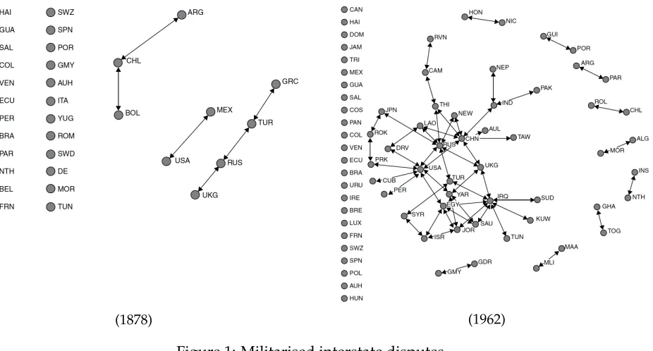
To illustrate this, take a look at the set of Militarised Interstate Disputes between states1in 1878

– the year when the Congress of Berlin ended the Russo-Turkish War – and the type of relations in

(1878) (1962)

Figure 1: Militarised interstate disputes

Source:Networks of Nations: The Evolution, Structure, and Impact of International Networks, 1816-2001, (Maoz, 2010)

1962 – the height of the Cold War–, depicted in Figure 1.

In both periods of time the overall conflict structure within states is represented by networks of

bilateral conflicts. In 1878, the structure of disputes was characterised mainly by a network with

line components in which a state had at most two different conflicts at the same time. In 1962 the

picture is different, whilst there is a non-negligible number of isolated bilateral conflicts, there is

a less trivial cluster of nodes centred around military powerful and/or resource rich states like

the United States, Russia, China, or Iraq among others. It conceptually is hard to judge whether

it was the strength of Russia that made other countries engage in conflict with the US, or whether

they did so in order to oppose the threat that a potential US hegemony meant to them. In the

literature on International Relations, the former is broadly comprised by the termBandwagoning,

while the latter is frequently referred asBalancing(Waltz, 1979). The paper at hand sheds light on

this question in a stylised setting.

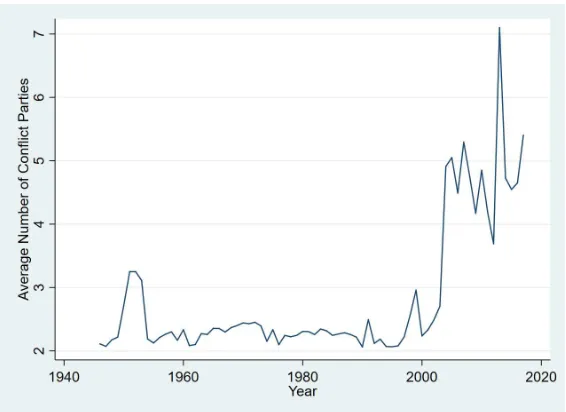
While the number of Militarised Interstate Disputes have declined over the second half of the

20th century, the was a sharp increase in internal and internationalised internal conflict. These

types of conflict are often referred to as civil wars and include recent examples like the Syrian war,

the civil war in Ukraine and the Colombian conflict.2 As figure 2 suggests, the number of parties

in military conflicts has increased on average over time, with the sharpest increase happening

2

Figure 2: Violent Conflicts Involve More Parties Over Time

after 9/11. Since every additional agent can have conflicts with multiple agents in the network,

the increase in conflictual links is likely to be even more pronounced, giving rise to the study at

hand.

We propose a setting in which there is an exogenous structure of bilateral conflicts across n

opponents as in Franke and ¨Ozt ¨urk (2015) (from heron F ¨O). Each link between a pair of players

represents a bilateral conflict. While F ¨O considers cases of symmetric characteristics, we allow

for heterogeneity between opponents in terms of their efficiency of conflict investment and the

valuations of winning, within and between different conflicts. We model conflict using a contest

success function based on the axiomatisation proposed by Skaperdas (1996). Finally, we induce

a trade-off between different conflicts through a budget-constrained cost function – following the

formulation proposed by Kovenock and Roberson (2012a), which can accommodate two canonical

cases already studied in the literature: i) pure cost convex case andii)budget constrained case.

The latter yields to the fact that military budgets can hardly ever be altered in the short run when

conflicts were not anticipated.

We show that a unique and interior Nash Equilibrium exists in the pure cost case, independently of

the model parameters. In contrast, in the budget constrained case the uniqueness and interiority

of the equilibrium rely on the spread of valuations a player holds for the different conflicts she

is involved in and the characteristics of the impact function. In line with F ¨O, we show that a

We thus use implicit methods to investigate some local effects of the asymmetries between the

players’ characteristics. We find that asymmetries in the prizes leads to Bandwagoning behaviour,

mainly driven by the interaction of local network externalities induced by the conflict structure.3

If there are players of different strength, as indicated by their efficiency to transform resources into

winning probabilities, players tend to fight opponents more strongly that are similar with respect

to their strength. Finally, we investigate the changes in the strategies due to heterogeneity in the

number of conflicts of a player’s opponents. We find that more central players tend to be fought

more fiercely.

Related Literature: Modelling conflict on networks is a relatively recent stream of research in

economics (Dziubi ´nski et al., 2016), starting with the model proposed by Franke and ¨Ozt ¨urk

(2015). The authors define a model where players are embedded in a network of bilateral

con-flicts and each player chooses the amount of resources that they want to invest to each conflict.

The conflict is modelled using a lottery success function. The trade-off between different conflicts

is induced through a convex cost function of the total amount of resources employed. They relate

the total conflict investment with the player’s number of conflicts. The article focusses on

ag-gregate behaviour and thus abstracts from individual characteristics by assuming symmetry with

respect to all model parameters.

Beside the seminal paper by Franke and ¨Ozt ¨urk (2015) and the subsequent studies looking at this

type of environment (e.g. K ¨onig et al., 2017; Dziubi ´nski et al., 2017; Matros and Rietzke, 2018)4

there are different fields that are related to the paper at hand. The key distinction between our

paper and the afore-mentioned (among other differences) is that the players choose an effort level

for each opponent they share a link with, rather than choosing a single effort that they employ

against all players.5 _{Settings with link specific actions, not necessarily conflict or contest though,}

are quite recent. To the best of our knowledge in addition to Franke and ¨Ozt ¨urk (2015) the only

models on games on networks that introduce multidimensional strategies are Goyal et al. (2008)

or Bourl`es et al. (2017). In analysing heterogeneity of players and their response with respect to

specific opponents, this characteristic is crucial.

3

Klose and Kovenock (2015) refer to these as identity-dependent externalities. The first formalisation in contest to our knowledge can be found in Linster (1993).

4_{Huremovic (2016) studies as well conflicts on networks but with a different perspective. He is interested in the} endogenous network formation of a network of conflict.

Apart from that, our paper is related to the literature on multi-battle contests based on the

canon-ical Colonel Blotto game. The Colonel Blotto game has been studied extensively since its first

formulation by Borel (1921), where two players need to allocate simultaneously a finite number

of resources overkdifferent battlefields, the outcome over each battlefield is modelled as an

all-pay-auction. This specification is well-researched with characterisations of heterogeneity between

players, complementarity of prizes and other modifications to the standard formulation (Borel

and Ville, 1938; Gross and Wagner, 1950; Laslier, 2002; Roberson, 2006; Hart, 2008; Hortala-Vallve

and Llorente-Saguer, 2012; Weinstein, 2012; Kovenock and Roberson, 2012a; Kovenock et al., 2015;

Macdonell and Mastronardi, 2015; Thomas, 2018).

Using a lottery to determine the outcome in each battlefield following the Tullock (1980)contest

success function, where the probability of winning a specific battlefield is a non-decreasing function

in the own resource allocation and decreasing in the enemy’s allocation, is another approach to

the two player Colonel Blotto problem. Based on thiscontest success function, Friedman (1958) is

able to characterise the equilibrium in pure strategies of the two-player game with symmetric and

asymmetric budgets and battlefield valuations. The main result of that study is that the optimal

allocation is proportional to the valuation of the prizes.6 This result is a special case of our model.

This strand of the literature relies on models with only two players. Our paper is a contribution to

the theory of contests in which we extend the current set of models by considering a multi-player

environment with asymmetric efficiency of resources toward the conflict outcome and conflict

prizes. This variation allow us to find new insights about the effects of the interactions of local

network externalities across different conflicts.

We also add to a debate in the literature of international relations. In a war and many other

con-flictual settings, there is no (strong) institution that allows parties to come to a peaceful agreement.

This state can be referred to as Hobbesian anarchy, due to Hobbes (1998). It is the law of the Jungle

that should determine the winner(s) in such a state. Differences in the parties’ strengths should

thus be crucial to any analysis of conflict. Early on, Waltz (1979) and Walt (1987) coined the terms

BalancingandBandwagoning. Balancingis a behaviour where weaker parties ally to balance the

power of a strong common opponent. Bandwagoningrefers to the case where weak parties rally

behind the strategic goals of the hegemon. There has been an ongoing discussion about which

of these is more likely to occur in situations of armed conflict.7 Our model allows to introduce

a hegemon into the model, using different measures of strength, in order to shed light on the

6

Robson (2005) generalises it by allowing the contest success function to include an effectiveness advantage and idiosyncratic noise.

behaviour of the remaining players.

The rest of the paper is structured as follows. In the next section, we describe the setup of

the model and discuss some its properties. In Section 3, we prove the uniqueness of an interior

Nash Equilibrium, discuss some of its properties and show the non-existence of a general explicit

algebraic solution to the model. In section 3.1, we study the specific family ofk-regular network

structures that enables us to have sharper predictions regarding the equilibrium behaviour. In this

section we also present some comparative statics. In section 3.2, we present results concerning the

asymmetries coming from the network structure. Section 4 concludes.

2

The Model

LetI = {1, . . . , n}be a finite set of players withn ≥ 3. All battlefields are contained inB ⊆ I2

where I2 is the set of unordered pairs of I with typical element (ij). The underlying conflict

network G is represented by the connected graph associated with the pair of sets (I, B).8 We

say that any pair of players i and j is involved in a bilateral conflict on battlefield (ij) if and

only if(ij) _∈ B. The network G is undirected (∀{i, j_} : (ij) _∈ B _⇔ (ji) _∈ B) and irreflexive

(∀i _{∈ I} : (ii) _6∈ B). LetNi = {j ∈ I|(ij) ∈ B} denote the set ofi’s rivals. The total number of

rivals ofiis given bydi =|Ni|. The setN˜i ={1, ..., di}then uses the opponent orderingeij, which

is the row number of each element of the ordered vectorNifromjlow to high. The total number

of battlefields is 1₂bwith b = P

idi = |B|. Notice, that every player has at most(n−1)rivals and, consequently, the networkG contains at most n(n₂−1) battlefields. In each bilateral conflict,

(ij) _∈ B, players i and j fight for a strictly positive exogenous prize. Player i’s valuation of

winning the prize against playerj is denotedvij. This framework can accommodate

constant-sum bilateral conflicts, whenvij =vji, or non constant-sum bilateral conflicts, whenvij 6=vji.9

Each playerican allocate an amount of resourcesxij ∈ R+ in order to increase her probability

of winning battlefield (ij) against playerj. Thus, x_{i = (xe}

ij)j∈Ni is adi-dimensional vector that contains all effort choices of playeri.

The outcome of each bilateral conflict is determined by the total amount of resources allocated to

8 _{A graphGis connected if for every pair of players iandjinN there exists a path between them. We do not} consider disconnected network structures. The results that we are presenting hold for any non-trivial component of any disconnected network. A path in a networkGbetween nodeshandlis a sequence of linksi1i2, i2i3, . . . , ik−1ik

such that everyimim+1∈Bfor eachm∈ {1, . . . , k−1}, withi1=handik=l. Each node in the sequence{i1, . . . , ik}

needs to be distinct. 9

that specific battlefield. Playeri’s probability of winning is determined by acontest success function

(from hereon CSF) p(aixij, ajxji), where ai ∈ R++captures how efficiently player ican employ

her resources to increase this probability. The CSF is increasing and concave inxij and decreasing

and convex inxji.10Further, it does not depend on anyxlkwith(lk)6= (ij). The axiomatised class

of CSFs by Skaperdas (1996) satisfies these properties. Thus, the probability ofiwinning the prize

in the battlefield againstjobtains as

˜

pij = ˜p(aixij, ajxji) = 

 

 

f(aixij)

f(aixij)+f(ajxji) if (xij +xji)6= 0

p_ij if (xij +xji) = 0

(CSF)

wherep_{ij ∈}(0,1)is the tie breaking rule. The impact functionf(.)is a twice differentiable, positive

and strictly increasing function of its argument withf(0) = 0.

The tie breaking rule is defined exogenously in order to define the CSF at(0,0). Since this might

cause problems for some of the results we intend to show, we use the fact that

˜

p(aixij, ajxji) = lim δ→0

f(aixij) +kδ

f(aixij) +f(ajxji) + (1 +k)δ

The limit of this function coincides with our previous definition at every point. Even the tie rule

can be set flexibly since

lim

δ→0

f(aixij) +kδ

f(aixij) +f(ajxji) + (1 +k)δ

xij=xji=0

= lim

δ→0

kδ (1 +k)δ =

k

1 +k ∈(0,1)

for everyk ∈ (0,∞). This approach is essentially the one suggested in Myerson and W¨arneryd

(2006) with the slight adjustment to accommodate more flexible tie breaking rules. The function

we intend to use as contest success function is thus

p(aixij, ajxji) =

f(aixij) +kδ

f(aixij) +f(ajxji) + (1 +k)δ (1)

for some arbitrarily smallδ >0.11

For ease of notation, throughout the rest of the paper, letω = (v, a)be the combination ofbvalues

collected inv and then population weights collected ina. The space of all such combinations

10

This translates into the following condition onf():f′′_(a

ixij)(f(aixij) +f(ajxji))−2f′(aixij)<0. In words,f()

can have any degree of concavity but should not be too convex. 11_{Note that this impliesp}

ij+pji6= 1fork6= 1. Alternatively one could assumek= 1implyingpij=

1

2, resulting in

isΩ _∈ Rb+n

++. We call the case where all valuations across players and battlefields and all

effi-ciencies across all players are the same astrictly symmetricparameterisation and denote itω. Let

Ω =_{(λ1111b, λ2111n)|(λ1, λ2)∈R2++}denote the set of all such parameterisations.12

Players incur costs for employing resources which are captured byC(Xi)whereXi =Pj∈Nixij

denotes total resources spent by a player across all her battlefields. We consider abudget-constrained

cost-basedframework as the one proposed by Kovenock and Roberson (2012b) such that for some

R >0, we have

C(Xi) =   

 

c(Xi) if Xi≤R

∞ if Xi> R

(2)

The properties ofc(Xi)determine the magnitude of opportunity costs for playeri. If the function

is strongly increasing at some level ofXi, she will have to withdraw resources from other

battle-fields rather than increasing the total amount of resources spent. In general,c(Xi)is continuous,

non-decreasing and convex. We use c′(0) = 0 for proving our results but they go through for

sufficiently small c′(0) > 0 as well. This definition of the cost function allows the study of two

canonical formulations. In the budget-constrained case(BCC) the cost function is c(Xi) = 0for all

Xi. In this case the opportunity costs across battlefields are mediated solely through the curvature

properties of the CSF. Since the marginal returns on each battlefield are strictly increasing in own

allocated resources, each player exerts the total amountXi =Racross all battlefields.

The second case is thepure cost case (PCC) in whichRis arbitrarily large, such that we can

guar-anteeXi < Rin equilibrium for each playeri. The opportunity costs for each battlefield enter the

model through the positive cross derivatives ofc(Xi)which in this case is assumed to be strictly

convex.

For technical tractability we ignore the mixed case in which there is a non-trivial cost function

c(Xi)and potentially binding constraints for some players but not all players.

For each battlefield(ij)_∈B, agenti’s expected pay-off isuij :R+×R+→R+such thatuij =pijvij.

We assume that agents are expected pay-off maximisers with risk-neutral preferences. We

con-12₁₁₁

sider an additively separable utility function given by13

Ui(xi,x−i,G) =

X

j∈Ni

uij −C(Xi)

The set of players, the network structure, the action spaces and expected payoffs define a

simul-taneous game. Our objective is to study the Nash equilibrium of this game and how the

char-acteristics of the network structure, distribution of values and assumptions on the cost function

influence the equilibrium behaviour.

3

Equilibrium Analysis

Given the above structure, each player faces the following maximisation problem of dimensiondi

determined by the network structureGfor givenx_−i,

max xi∈Rdi+

Ui(xi,x−i,G) with a givenx−i∈Rb+−di (3)

In the pure cost case, the equilibrium behaviour is described by the balance of marginal benefits

and marginal costs for each battlefield(ij)_∈Band every playeri_{∈ I}

aif′(aixij)f(ajxji)

(f(aixij) +f(ajxji))2

vij =C′(Xi) (PCC)

In the budget-constrained case, when the properties of the cost function induce the opportunity

costs through a fixed budget that needs to be spent, the optimal allocation of resources for each

playeri∈ I for every battlefield(ij)∈B in equilibrium is characterised by

f(aixij) +f(ajxji) P

k∈Ni[f(aixik) +f(akxki)]

=

p

vijf′(aixij)f(ajxji) P

k∈Ni p

vikf′(aixik)f(akxki)

(BCC)

Players’ marginal benefits are shaped by the resource allocation of their direct rivals but also

the rivals of their rivals and so on. This interdependency induced by the cost function determines

how an individual reacts to changes in some of the parameters of the environment. Some of the

behavioural implications thus occur even though a player’s preferences are not directly altered.

F ¨O asserted that a unique equilibrium exists irrespective of the network structure if the players

characteristics in terms of their preferences and technologies are homogenous. In the setting of

convex costs, this homogeneity is not needed to guarantee uniqueness. Under a strict budget

con-straint we can guarantee it by staying in an open neighbourhood around symmetric parameters.

With the CSF as defined in (1), the game is a continuous game with a finite set of players and

com-pact strategy spaces. Thus, we can apply the theorems due to Debreu (1952), Glicksberg (1952)

and Fan (1952) in order to guarantee the existence of a pure-strategy Nash equilibrium. Due to

the continuity of the cost function and the (almost) infinite marginal gains close to(0,0)on each

battlefield, equilibria are strictly interior. If that is given, the system of first order conditions (from

hereon referred to asF) characterises these equilibria. We show that the determinant of that

sys-tem is always strictly larger than zero. This provides us with the following result.

Proposition 1(Pure Cost Case).

For the pure cost case, a unique, interior pure-strategy Nash equilibrium exists. The solution function

x(ω) : Ω7→Rb

++has the following properties:

• It is of classC∞

• Its derivative is given byDx(ω) =−[DxF(x(ω);ω)]−1DωF(x(ω);ω)

The budget-constrained setting is slightly more complicated, as players cannot increase or

de-crease their total effortsXi to any other level thanR. We need to ensure that every player can

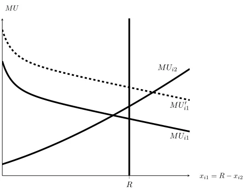
equalise marginal returns across battlefields. Consider Figure 3. A playerifor whichdi = 2can

pin down her decision on both battlefields by choosing onlyxi1 since xi2 = R−xi1. The figure

shows her marginal utilities on both battlefields. Since they are both decreasing in the respective

effort, marginal utility on battlefield 2 is increasing inxi1.

With M Ui1 player ihas enough endowment to balance marginal utilities, that is, to reach the

intersection of the two functions. If we increase the battlefield value fromvi1tovi′1, as is shown by

the dotted lineM U_i′₁, it would be optimal to spend all resources on the battlefield with the higher

marginal revenue and we obtain a corner solution.

Since the marginal utilities increase in the valuations and efficiencies, this also restricts the relative

values vi1

vi2 and efficiency parameters (i.e. ai andaj). This mutual restraint can be characterised

R

M Ui1

M U′ i1

M Ui2

xi1=R−xi2

M U

Figure 3: Marginal Utilities for a Player with 2 Battlefields

Take some playeri _{∈ I}and denote the highest valuation she holds with vih = max{vij|j ∈ Ni}.

The highest marginal utility that playerican get in the battlefield againsthwhenxih=Ris

max

xhi≤R

∂Ui(xi,x−i,G)

∂xih

xih=R

=    1 4

aif′(aiR)

f(aiR) vih if ai ah ≤1 aif′(aiR)f(ahR)

(f(aiR)+f(ahR))2vih if ai ah >1

Since the first order condition of this problem is given by

∂Ui(xi,x−i,G)

∂xih∂xhi

= aiahf

′_(a

ixih)f′(ahxhi)(f(aixih)−f(ahxhi))

(f(aixih) +f(ahxhi))3

!

= 0

the argument that solves it isxhi= _aa_hixih, meaning that the highest marginal utility for a specific

battlefield is achieved when winning probabilities are the same for both players.

Equally well, on the battlefield whereiholds the lowest valuationvil = min{vij|j ∈Ni}, we can

find the minimal marginal utility under any profile wherexih=Ras

min

xli≤R

∂Ui(xi,x−i,G)

∂xil

xil=0

= aif

′₍₀₎

f(alR)

vil

When this marginal utility (denote itM Uij for some battlefield(ij)) is larger than the one on

(ih)whenxhi= min{_aa_hixih, R}= min{_aa_hiR, R}, then playerihas an incentive to divert resources

min

xli≤R

∂Ui(xi,x−i,G)

∂xil

xil=0

> max

xhi≤R

∂Ui(xi,x−i,G)

∂xih

xih=R

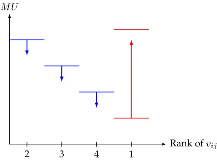
To complete this argument of the proof, one has to notice that forxih = 0andxhi = R, we have

M Uih ≥ M Uik for all k =6 h. This implies that each player can achieve M Uij = M Uik for all

{j, k} ∈Ni.

M U

Rank ofvij

2 3 4 1

Figure 4:M Uihcan be equalised with allM Uij

Note: Valuations are ordered from high to low, i.e. 1 represents

If that holds, we can use the same techniques as in the former proof to obtain the following

result.

Proposition 2(Budget-Constrained Case).

If for alli∈ I we have

vil

vih

> 1 4

f(alR)

f(aiR)

f′(aiR)

f′₍₀₎ (4)

then for eachω_∈Ωa strictly interior, unique pure-strategy Nash equilibrium exists.

The solution functionx(ω) : Ω_7→Rb

++has the following properties:14

• It is of classC∞_.

• Its derivative is given byDx(ω) =−[DxF(x(ω);ω)]−1DωF(x(ω);ω).

14

This is a slight abuse of notation. Technically, the function isx˜(ω) : Ω7→Rb+n

++. The shadow prices of increasing

the total amount of effortsλis an output of that function for alli ∈ I. Here, we construct the function from theb

Therefore, the interplay of battlefield values, the initial endowment and properties of the the

impact functionf(.)determine whether the game has a unique Nash equilibrium. Note that the

caseai =aj = 1andvij =vji=v >0for all(ij)∈Balways fulfils the condition.

The analytic condition is particularly interesting as a familiar assumption made in economics

could guarantee existence for all kinds of parameters. If we assume that the impact of the first

marginal effort increase is infinitely large, that islimx→0f′(x) =∞, there is no bound on budgets

and valuations anymore. While we do not intend to use this assumption for the rest of the paper, it

relates to common assumptions made in economics like theInada-conditionin production or utility

functions. One could state it as the first marginal unit sent to a battlefield having a large impact

compared to a further unit sent when there are already many on the field.

Games played on networks give rise to a complex set of dependencies. Any attempt to solve for

equilibria should reflect this for the model at hand. The following result tells us that to solve

explicitly the system of first order conditions, we need to express the best response functions of

some playerias functions of a player’s strategies that does not share a link withi.

Lemma 1.

There exists an indirect global dependence where for any pair of agents h and l who are not rivals (i.e.

h6∈Nlandl6∈Nh), the effort levels as characterised by the system of first order conditions can implicitely

be expressed asx_h∗₍X∗

−{h,l},xl∗)andxl∗(X∗_−{l,h},xh∗).

In that sense, the fact that we have a connected network creates indirect relations between all

players throughout the rivals of rivals along any path of the network. This does not mean that

players “respond” to distant players as the word best-response function suggests. It is merely a

mathematical fact that we use to show that an algebraic solution for the equilibria can be obtained

for hardly any network structure. How much any player’s actions affect another player’s effort

levels in equilibrium depends on how long the shortest possible path between them is. Consider

for example a line network with 6 players in a budget constrained setting. In this case the two

players in the ends allocate all their resources in their unique battlefield. Let playeribe one of

the end players in the line. Based on Lemma 1, we can mathematically express any of her best

responses asx∗_ij =xij(xjk(xkl(xlp(xpq))))as illustrated by Figure 5.

i j k l p q

Figure 5: Line Network with 6 Players

a sum. Therefore, to find the equilibrium strategies, we require to find the roots of at least one

general polynomial of degree25.

Denoting the length of the longest path in a given network withL, solving the system of first order

conditions for all players, generally requires us to find the roots of at least one general polynomial

of degree2L_{. This is a mathematical impossibility for any degree greater or equal to 5, according}

to the Abel-Ruffini Theorem (1779).

Corollary 1.

The equilibrium strategies of the game do not have a generic algebraic solution if the length of the longest

path between any two players is greater than or equal to3.

By a generic algebraic solution we mean any formula which would express the roots of the

polynomial as functions of the coefficients by means of algebraic operations (i.e+,−,×or/) and

roots of natural degrees. This is the reason for employing more implicit methods when analysing

equilibrium behaviour, or more specifically, changes in equilibrium behaviour that correspond to

changes in parameters. Also, we need to restore some degree of symmetry that we impose on the

network structure.

3.1 k_{-Regular Networks}

Propositions 1 and 2 provide the general form of the matrix of derivatives for any unique

equilib-rium. If we focus our attention on a subset of network structures, it is possible to obtain closed

forms of these matrices to assess comparative statics more precisely. As these expressions appear

more often in the subsequent part of the paper, denotep1_ij =p1(aixij, ajxji)as the derivative ofpij

respect to its first argument,p2_ij =p2(aixij, ajxji)the derivative ofpij respect to the second

argu-ment. The second and cross-derivatives are equivalently given byp11

ij = p11(aixij, ajxji) = −p22ji andp12_ij =p12(aixij, ajxji) =−p21ji. The set of graphs we consider is defined as follows.

Definition.

Ak-regular network is any graph for whichdi=kfor alli∈ Iand somek∈ {2, ..., n−1}.

This family of graphs includes the complete network (k = n₋1) and the ring (or minimal

connected) network (k= 2) as well as some networks in between these extreme cases as illustrated

by Figure 6 for the case ofn= 6.

Within these networks it is possible to characterise the equilibrium strategies in case of a

1

2

3 5

6

4

(a)k= 2

1

2

3 5

6

4

(b)k= 3

1

2

3 5

6

4

(c)k= 5

Figure 6: Examples ofk-Regular Networks forn= 6

class of graphs and the equilibrium efforts exerted. This means that, even though in a relatively

restrictive set of cases, we are able to infer the exact network structure from the strategies played.

Lemma 2.

Ifω∈Ωthe following holds:

The graph isk-regular fork_≤n₋1if and only if the equilibrium for alli_{∈ I} isxij =xs > 0for all

j _{∈ I\{}i_}.

This equilibrium obtains as

xs= 1 kC

′−1_(p1_(axs_{, ax}s_)av)>0

This result might be useful, as often in real world conflicts effort levels, in the form of soldiers or

monetary contributions, are more observable than the underlying network structure. Note that a

symmetric equilibrium in ak-regular network does not necessarily imply thatω∈Ωthough. The

condition for a strategy profilexs_{to constitute an equilibrium in such a network is}

p1(aixs, ajxs)

p1_(a

kxs, alxs)

= vkl vij

for all (ij),(kl) _∈ B, which can be satisfied forω /_∈ Ω. If we restrict the degrees of freedom

further there is some deductions one can make about the parameters as well.

Corollary 2.

choiceR_k ≥xs_{>0for alli∈ I it follows that}

aj =ai ⇔vij =vji ∀i, j∈ I

Probably the most frequently used CSF is the one suggested by Tullock (1980) for whichf(x) =

x. With the above we can have a first glance at potential comparative statics with respect to

pa-rameters.

Example 1(Relative Battlefield Values).

Let every player in ak-regular network have an endowment equal to one and values such thatvij =vjifor

all(ij)_∈B. AlsoV =P

j∈Nivij for alli∈ I. In a budget-constrained setting, the equilibrium behaviour

will be given by

For alli∈ I and every(ij)∈Bthe optimal allocation strategy isx∗_ij = Pvij

k∈Ni

vik

When instead of facing a budget constraint, the opportunity cost of allocating resources is induced by a

cost function, we observe the same equilibrium strategy if it is of the formC(Xi) = 1₄XiV. The degree of

convexity of the cost function thus needs to be proportional to the total value of the contest to each player.

Since all involved functions are continuous in their respective arguments, we might infer that increases in

own value increase an agent’s effort, while those values winning over her decrease it.

Notice, that if we have an environment where players are symmetric and all dimensions (i.e. endowment,

battlefield values, number of rivals), our setting collapse to the same equilibrium behaviour already found

previously in the literature by Friedman (1958). In there the network structure starts to be redundant and

only the relative battlefield values will determine the amount of resources allocated to a given conflict. If

all valuations are multiplied by the same constant, strategies do not change. Following up on the notion of

externalities, this illustrates why it does not matter how much individualihates individualj(vij high). If

individualkis hated more (vik > vij), it appears as ifirelatively likesj. This is also in line with observing

conflict even in very cohesive groups like tribes and families.

In a symmetric equilibrium within a k-regular network, the first order conditions are the same

for every player sinceXi =kxs. Thus, we can do a comparative static analysis on the symmetric

equilibriumk-regular effort choice with respect to the parameters. Note that this is different from

change a particular parameter, rather than the joint value for all player for that parameter.

∂xs ∂a <0,

∂xs ∂v >0,

∆xs ∆k <0

The effect of increasing everyones’ valuations should be correctly anticipated. If we move from

one symmetric equilibrium to the next along a linear increase of all efficiencies we do see a

reduc-tion in individual efforts. The same holds if the degree kincreases for all players. The marginal

change in total effort,X=nkxs_{, is proportional to the first two expressions. Thus, we can say that}

it increases in valuations and decreases in efficiencies. Notice though that reduced efforts through

increases in symmetric efficiencies should not be confused with what could be coinedeffective

ef-forts x˜ij = aixij. For instance in a war between countries, although less soldiers are sent to the

battle by each agent, the battle intensity could increase since the weapons got more powerful. We

find the same result as F ¨O related to the degree of the network (i.e. total effort increasing ink),

which should not be too surprising as we are in a strictly symmetric setting.

We stop investigating symmetric changes of parameters here, as this paper is concerned with

asymmetries in networks of conflicts. In Proposition 1 and 2 we already gave an abstract

charac-terisation of the derivatives at any given equilibrium. In the the setting ofk-regular networks, we

can provide general algebraic expressions that allow us to perform comparative statics for which

we know the signs and magnitudes.

Proposition 3.

In ak-regular network the partial derivatives around the equilibrium at an arbitrary symmetric

parametri-sationω_∈Ωcan be obtained analytically as

∂xij

∂vij

=−z−(k−1)C ′′_(X)

z₋kC′′_(X)

ap1 z >0 ∂xil

∂vij

= C

′′_(X)

z−kC′′_(X)

ap1

z <0 for alll6=j ∂xij

∂ai

=₋ 1 +z z₋kC′′_(X)

p1_v

z + xs

a

IfX_→Rwith the cost function defined in 2, these become

∂xij

∂vij

=−k−1

k p1 ap11_v >0

∂xil

∂vij

=−1

k p1

ap11_v <0 forl6=j

∂xij

∂ai

= 0

Let us consider the comparative statics of valuations first. For this it is more illustrative to

con-sider the budget-constrained case. As expected, a player increases her effort on a battlefield as her

corresponding value increases. In the constrained setting, she must therefore shift resources from

other battlefields. Since these other battlefields are still symmetric with respect to the respective

valuations, the reductions in efforts are symmetric. Intuition would thus let us to believe that ∂xij

∂vij + (k−1) ∂xil

∂vij = 0. That is in fact the case.

If we observe the pure cost case, this trade-off is mediated by the convexity ofC(·). IfC′′(X)→0,

the player just increases her effort on(ij) without reducing it anywhere else. IfC′′_{(X) → ∞we}

do in fact end up with the constrained solution.15

The efficiency parameters cannot make a difference to the effort distribution in the budget-constrained

case since the marginal change applies symmetrically to all battlefields and makes us end up in

the same symmetric equilibrium for a givenkandR. In the pure cost case it is interesting to note

that the sign of the effect of an efficiency increase is not clearly defined for all cases. For the class

of impact functions that are homogenous of degreer(within the class axiomatised by Skaperdas

(1996)) one can show that both signs are indeed possible.

Proposition 4.

Letf(ax) = (ax)rforr_∈(0,2)16_{andC(X) =} 1

2X2. Then we have

∂xij

∂ai

<0 for r= 1

∂xij

∂ai

>0 for r_→0

∂xij

∂ai

>0 for r_→2

15_{This convergence result assumes thatC}′′_(X)

is continuously differentiable. Since we obtained the results indepen-dently from solving the constrained optimisation of 3, this is not necessary and just an additional observation.

There are two competing effects that determine the sign: (i) the opportunity to reduce costs

al-lows each player to maintain the same probabilities on each battlefield while lowering total costs

and (ii) the increased efficiency increases marginal probabilities on each battlefield, thus creating

an incentive to increase efforts.

Interestingly, the effect that any change has on the rest of the network seems to be independent

of this sign. This is due to the fact that the slope of the best response functions, implicitly

charac-terised by the FOCs, is proportional to the cross-derivatives of the CSF on that battlefield. Since at

any equilibrium in whichaixij =ajxjiwe havep12ij =−p21ji andp12ij =p21ji, which impliesp12ij = 0.

Since one can show that this is a maximum with respect toxji, playeriwill reduce her effort ifj

changes her effort in either direction.

Proposition 5.

Fix somek-regular networkG. Letω′ _{=ω+ (}0_,1_{iiǫ)for someω ∈ΩandS = (I}′_{, B}′_{)⊆Gsuch thatS}

is a complete network. If there exists someǫ > 0such thatω′ ∈V(ω)and the equilibriumx(ω′)satisfies

xij(ω′)≶xsfor all∈ I′\{i}, then

xji(ω′)< xs

xjk(ω′)> xs

Furthermore, if we define∆xlq =xlq−xs, we have

∆xij >∆xji,∆xjk

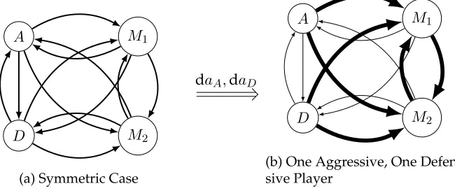
In words, irrespective of whether she becomes more or less aggressive, the other players in the

network reduce their efforts towards her.

Figure 5 illustrates what happens in case one player becomes more aggressive (playerA), while

another reduces her efforts against her opponents (player D).17 _{The magnitude of the arrows}

between players indicates the relative level of efforts.

Panel (a) of the figure represents the symmetric case in which all efforts (arrows) are of the same

magnitude. Choosing daAand daD such that the indicated changes in A’s andD’s effort follow,

we see in panel (b) that the two remaining players concentrate their efforts against each other.

17

A M1

D M2

(a) Symmetric Case

daA,daD

A M1

D M2

(b) One Aggressive, One Defen-sive Player

Figure 7: Diagrammatic Representation of Proposition 5 fork= 3

Note: The size of the arrows refers to the relative amount of resources allocated in each bilateral conflict. Throughout the rest of the paper, numbers will indicate numerical observations, while different sizes of arrows indicate actual

results.

Given a specific level of costs that is prohibitive (or a strict budget constraint), efficiencies become

a scaling factor of effective budgets. Since after applying the change it must be that eitheraA> aD

or aA < aD, one can interpret the above figure in terms of the fight of rich against the poor.

The prediction of the model at hand is that conflict intensity contracts towards the mediocrely

endowed individuals and away from the rich and the poor. If efficiency is a measure of strength,

the model suggests that the weaker players will rather fight each other in a situation where a

single player is stronger than the rest. While Bandwagoning in typically needs the weak to rally

behind the strong player who in turns fights them less/ceases to fight them, Balancing (i.e. the

weak teaming up to oppose the strong) is not the strategically optimal behaviour.

While any change in efficiencies bears a certain degree of symmetry with it, since∂ai is the same

for all(ij), a change in valuations induces more asymmetric strategic responses.

Proposition 6.

Fix somek-regular networkG. Letω′ _{= ω+ (1}

ijǫ,0)for someω ∈ ΩandS = (I′, B′) ⊆ Gsuch that

Sis a complete network.18 _{There exists someǫ >0such thatω}′ _{∈V(ω)and the equilibriumx(ω}′_{)for all}

k_{∈ I}′_{\{i, j}satisfies}

xij(ω′)> xs> xik(ω′)

xjk(ω′)> xs> xji(ω′)

xkj(ω′)> xs> xki(ω′)

(5)

18

In network terms:Sis a subgraph ofGinduced by the cliqueI′

Furthermore, if we define∆xlq =xlq−xs, we have

∆xij >∆xjk,∆xkj (6)

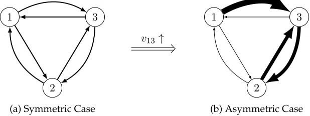
Figure 8 exemplifies this statement for the case of three players.

The effect of increasing player1’s value on her effort level against player 3 is intuitive. The effects

on playerj’s and all playerk’s efforts are less obvious. Roughly speaking, the effect of increasing

vij has a first-order effect only on player i’s effort levels and a second-order effect on all other

players. This is due to how the values feed into the players’ payoffs. While each own valuation

has a direct effect on her payoff, it can only affect other players’ payoffs through the strategic

channel. That is, the fact that even ‘impartial’ players change their equilibrium effort in case of a

change in some other player’s values is a result of the interdependencies of battlefields.

1 3

2

(a) Symmetric Case

v13↑

1 3

2

(b) Asymmetric Case

Figure 8: Diagrammatic Representation of Proposition 6 fork= 2

The behaviour of the preceding proposition, graphically depicted in Figure 8 is an even clearer

prediction of Bandwagoning behaviour as opposed to Balancing. Player 1 attacks player 2 more

aggressively and thus fights player 2 considerably less. Player two in turn does the same and

so they end up fighting player 3 jointly. Interpreting a high valuation as strength is a common

interpretation in the contest literature.19 This result could equally well be described as a form of

bullying, where one individual decides to bully a peer and so-called bystanders follow the bully

and become hacks. The fact that significant shares of adolescents are observed to behave in that

matter is well-established in social psychology (see for example Craig and Pepler (1998), O’connell

et al. (1999) and Salmivalli et al. (1996)).

3.2 Network Structure and Degree Asymmetry

The preceding comparative statics can be interpreted in terms of a strong player affecting the

whole network. So far we have looked at strength by considering the preference and technology

parameters. The degree centrality of a player ( i.e. the number of links she has to other players) is

another measure we could explore with that interpretation. Though we are leaving the realm ofk

-regular networks here, some of the symmetry features and the associated intuition are important

in these discrete comparative statics as well.

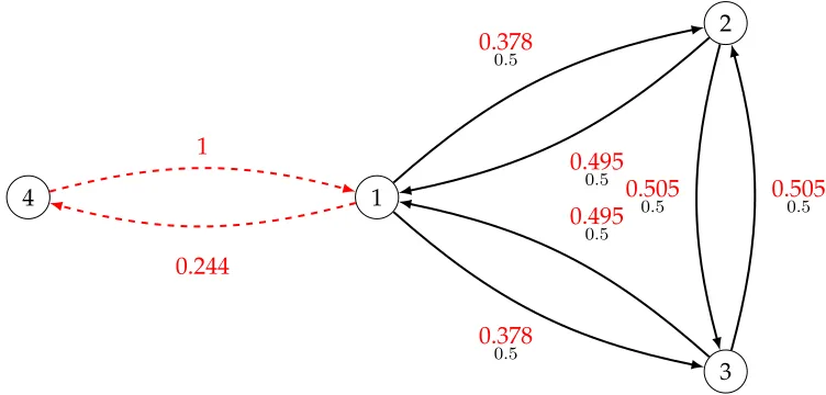
Example 2(Relative Network Structure).

Consider a budget-constrained setting in which every player has an endowment equal to one and faces

battlefields with the same valuev¯in each conflict. We introduce asymmetries solely a single player’s degree.

There are4players and one of them faces rivals with different degree.

4 1

2

3 1

0.244

0.378

0.5

0.495

0.5

0.495

0.5

0.378

0.5

0.505

0.5 0.5050.5

Figure 9: Example asymmetry due to the network structure with budget constraint

Note: Red figures indicate efforts when player 4 is linked to player 1. Black figures give the efforts when only players 1,2 and 3 are connected to each other.

In this network, player 1 chooses the same efforts against players2 and3. From her perspective these

two players are identical. Player4differs from them as she puts all her resources on(14). For player1this

means that the probabilityp12is bounded by above by1/2. Comparing this to our earlier results, it seems

that the number of rivals is weakening player 1on each battlefield. If the value on(14)is also given byv¯

though, her expected payoff in the 4-player game is higher than in the 3-player game (1.062¯v >v¯).

How many rivals a player’s rival has thus acts as another measure of strength. There is two

a symmetric parametrisation, every player allocates a strictly positive amount of resources to all

her battlefields. That implies that if the amount of battlefields that she is involved in increases,

her efforts can be no greater than with fewer battlefield. However, the way that she is going

to decrease them depends on the characteristics of her rivals and their rivals. To understand

how these forces interact with each other, we consider a simple environment with strict budget

constraint equal to one and a network that exhibit high asymmetry in the players’ degrees. One

such structure is the star network. The periphery players (p) allocate all their resources against the

central player (iorj) and the central player allocate the same amount of resources against all her

rivals, _d1_i or _d1_j.

i

p

p p

p

j

p

p p

p

p

0.165

0.25

0.165

0.25

0.165

0.25

0.165

0.25

0.135

0.2

0.135

0.2

0.135

0.2

0.135

0.2 0.135

0.2

0.34

0.322

Figure 10: Star networks of order5(left) and6(right).

The effect of the own degree is straightforward. The central players allocate resources inversely

proportional to their degrees. In the star network of order5for allp _∈ Ni we havexip = 1₄ and

for the star network of order 6 for all p ∈ Nj we have xjp = 1₅. In order to create some extra

variance in terms of the degree distribution while we keep the setting tractable, we joint the two

stars by adding a link between the two central players, as it is shown in Figure 10 by the dashed

line. In this casexij = 0.34,xip = 0.165,xji = 0.322andxjp = 0.135. Even though playerj has

the opportunity to win a prizes on one more battlefield than playeri, their payoffs are almost the

same (Ui = 1.080 > 1.081 = Uj) compared to the case where both star networks are in isolation

(Ui = 0.800 < 0.833 = Uj). This example shows that the number of battles a player is involved

can weaken her. Indeed, the pressure made by the rivals of my rivals is beneficial orthe enemy of

my enemy is(or at least can be)my friend.

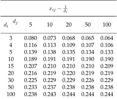
To understand the magnitude of this effect we can compare the equilibrium allocation with the

strategy coming from the heuristic _d1_i for different combinations ofdianddj, as it is presented in

equilib-xij −_d1_i

di dj 5 10 20 50 100

3 0.080 0.073 0.068 0.065 0.064 4 0.116 0.113 0.109 0.107 0.106 5 0.139 0.138 0.135 0.134 0.133 10 0.189 0.191 0.191 0.190 0.190 15 0.207 0.210 0.210 0.210 0.209 20 0.216 0.219 0.220 0.219 0.219 30 0.225 0.229 0.229 0.226 0.229 50 0.233 0.237 0.238 0.238 0.238 100 0.238 0.243 0.244 0.244 0.244

Table 1: Network comparative statics

rium strategies is always positive. This means that the amount of resources allocated to the rival

(i.e.j) with higher degree is always higher. Indeed, even thoughdiincreases for a givendj we

ob-serve a non-linear relation where the marginal increase has a decreasing effect over the difference.

This exercise suggests that in settings in which we can isolate the effect of own degree and rivals

degree, there is an initial effect related to the opponents’ degree leading playerito allocate more

resources against her. However, the changes in the magnitude are negligible with respect to the

rival’s degree changes.

4

Conclusion

We presented a model of conflict networks, focussing on heterogeneity of parameters and changes

in individual behaviour. Existence and uniqueness are discussed in a framework that

accommo-dates convex costs and budget constraints. In this framework it is possible to obtain comparative

statics with respect to effort efficiency, valuations and – in a more discrete fashion – the degree of

centrality of a player. We interpreted these results in terms of Bandwagoning – following a strong

player against her opponents – and Balancing – many weak(er) players joining forces to oppose a

strong(er) player.

The results seem to advocate Bandwagoning over Balancing, irrespective of the kind of strength

we consider. Since part of these considerations also have to do with threats that are dynamic in

nature, a full discussion of the two phenomena needs a model with multiple periods of

Endogenous network formation seems to be the natural next step, as strength should be at the

heart of the consideration with whom to start a fight. Since for standard methods like backward

induction, this requires to pin down payoffs, this is a technical challenge.

Providing the players with a conflict technology only, makes it hard to talk about the potential for

peace in this framework. Mutli-graph theory allows for two separate networks, one with conflict

and one with cooperative links. The opportunity costs of conflict generated by the opportunity of

cooperation can add a new perspective to this line of research. There is a recent, special interest

in this type of settings, following the work by Jackson and Nei (2015), Hiller (2017), and K ¨onig

et al. (2017). However, due to the complexity of applying multiple networks simultaneously, these

model either focus on endogenous network formation without an explicit allocation stage or on

unidimensional action spaces over an exogenous multi-layer network.

Finally, with sufficiently simple networks, it is possible to test how real entities behave under

cer-tain parameter constellations. First steps have been made in that direction, but there are many

References

BOREL, E. (1921): “La th´eorie du jeu et les ´equations int´egrales `a noyau sym´etrique. Comptes

rendus de l’Acad´emie des Sciences, 173(1304-1308), 58; English translation by Savage, L. (1953)

The theory of play and integral equations with skew symmetric kernels,”Econometrica, 21, 97–

100.

BOREL, E.ANDJ. VILLE(1938):Application de la theorie des probabilities aux jeux de hasard, reprinted in Borel E., Cheron, A.: Theorie mathematique du bridge a la portee de tous, Paris: Gauthier-Villars:

Paris: Editions J. Gabay, 1991 ed.

BOURLES` , R., Y. BRAMOULLE´, ANDE. PEREZ-RICHET(2017): “Altruism in networks,” Economet-rica, 85, 675–689.

CRAIG, W. M.ANDD. J. PEPLER(1998): “Observations of bullying and victimization in the school yard,”Canadian Journal of School Psychology, 13, 41–59.

DEBREU, G. (1952): “A social equilibrium existence theorem,”Proceedings of the National Academy

of Sciences, 38, 886–893.

DZIUBINSKI´ , M., S. GOYAL, AND D. E. MINARSCH (2017): “The Strategy of Conquest,” Cam-bridge Working Papers in Economics 1704.

DZIUBINSKI´ , M., S. GOYAL,ANDA. VIGIER(2016): “Conflict and Networks,” inThe Oxford

Hand-book of the Economics of Networks, ed. by Y. Bramoull´e, A. Galeotti, and B. Rogers, Oxford

Univer-sity Press.

FAN, K. (1952): “Fixed-point and minimax theorems in locally convex topological linear spaces,”

Proceedings of the National Academy of Sciences, 38, 121–126.

FRANKE, J. AND T. ¨OZTURK¨ (2015): “Conflict networks,”Journal of Public Economics, 126, 104 – 113.

FRIEDMAN, L. (1958): “Game-theory models in the allocation of advertising expenditures,” Oper-ations Research, 6, 699–709.

GLICKSBERG, I. L. (1952): “A Further Generalization of the Kakutani Fixed Point Theorem, with

Application to Nash Equilibrium Points,” Proceedings of the American Mathematical Society, 3,

GOCHMAN, C. S. ANDZ. MAOZ(1984): “Militarized interstate disputes, 1816-1976: Procedures, patterns, and insights,”Journal of Conflict Resolution, 28, 585–616.

GOYAL, S., J. L. MORAGA-GONZALEZ´ , AND A. KONOVALOV (2008): “Hybrid R&D,”Journal of

the European Economic Association, 6, 1309–1338.

GROSS, O.ANDR. WAGNER(1950): “A continuous Colonel Blotto game,” Working Paper RM-424. RAND Corporation, Santa Monica.

HARBOM, L., E. MELANDER,ANDP. WALLENSTEEN(2018): “Dyadic Dimensions of Armed

Con-flict, 1946–2007,”Journal of Peace Research, 45, 697–710.

HART, S. (2008): “Discrete Colonel Blotto and general lotto games,”International Journal of Game Theory, 36, 441–460.

HILLER, T. (2017): “Friends and enemies: a model of signed network formation,”Theoretical Eco-nomics, 12, 1057–1087.

HIRSHLEIFER, J. (1995): “Theorizing about conflict,”Handbook of defense economics, 1, 165–189.

HOBBES, T. (1998): “Leviathan,”Oxford: Oxford University Press, 21, 111–143.

HORTALA-VALLVE, R.ANDA. LLORENTE-SAGUER(2012): “Pure strategy Nash equilibria in

non-zero sum colonel Blotto games,”International Journal of Game Theory, 41, 331–343.

HUREMOVIC, K. (2016): “A Noncooperative Model of Contest Network Formation,” AMSE Work-ing Papers 21. Aix-Marseille School of Economics.

JACKSON, M. O. AND S. NEI (2015): “Networks of military alliances, wars, and international

trade,”Proceedings of the National Academy of Sciences, 112, 15277–15284.

KLOSE, B. AND D. KOVENOCK (2015): “The all-pay auction with complete information and

identity-dependent externalities,”Economic Theory, 59, 1–19.

K ¨ONIG, M. D., D. ROHNER, M. THOENIG,ANDF. ZILIBOTTI(2017): “Networks in conflict: The-ory and evidence from the great war of africa,”Econometrica, 85, 1093–1132.

KONRAD, K. A. (2009):Strategy and dynamics in contests, Oxford University Press.

KOVENOCK, D. ANDB. ROBERSON(2012a): “Coalitional Colonel Blotto games with application

——— (2012b): “Conflicts with multiple battlefields,” inOxford Handbook of the Economics of Peace

and Conflict, ed. by M. R. Garfinkel and S. Skaperdas, Oxford University Press, 266–290.

KOVENOCK, D., S. SARANGI, AND M. WISER (2015): “All-pay 2\ times 2 Hex: a multibattle

contest with complementarities,”International Journal of Game Theory, 44, 571–597.

LASLIER, J.-F. (2002): “How two-party competition treats minorities,”Review of Economic Design, 7, 297–307.

LIEBER, K. A.ANDG. ALEXANDER(2005): “Waiting for balancing: Why the world is not pushing

back,”International Security, 30, 109–139.

LINSTER, B. G. (1993): “A generalized model of rent-seeking behavior,”Public choice, 77, 421–435.

MACDONELL, S. T.ANDN. MASTRONARDI(2015): “Waging simple wars: a complete

characteri-zation of two-battlefield Blotto equilibria,”Economic Theory, 58, 183–216.

MAOZ, Z. (2010): Networks of nations: The evolution, structure, and impact of international networks, 1816–2001, Cambridge University Press.

MATROS, ALEXANDER, A. AND D. M. RIETZKE (2018): “Contests on Networks,” Economics

Working Paper Series. Lancaster University.

MYERSON, R. B.ANDK. W ¨ARNERYD(2006): “Population uncertainty in contests,”Economic The-ory, 27, 469–474.

O’CONNELL, P., D. PEPLER, ANDW. CRAIG(1999): “Peer involvement in bullying: Insights and

challenges for intervention,”Journal of adolescence, 22, 437–452.

P ´EREZ-CASTRILLO, J. D. AND T. VERDIER (1992): “A general analysis of rent-seeking games,”

Public Choice, 73, 335–350.

PETTERSSON, T. ANDK. ECK(2018): “Organized violence, 1989–2017,”Journal of Peace Research, 55.

ROBERSON, B. (2006): “The colonel blotto game,”Economic Theory, 29, 1–24.

ROBSON, A. W. (2005): “Multi-item contests,” Working Paper 1885-42587. Australian National

SALMIVALLI, C., K. LAGERSPETZ, K. BJORKQVIST¨ , K. ¨OSTERMAN, ANDA. KAUKIAINEN(1996): “Bullying as a group process: Participant roles and their relations to social status within the

group,”Aggressive behavior, 22, 1–15.

SANDLER, T. (2000): “Economic analysis of conflict,”Journal of Conflict Resolution, 44, 723–729.

SCHWELLER, R. L. (1994): “Bandwagoning for profit: Bringing the revisionist state back in,” In-ternational Security, 19, 72–107.

SKAPERDAS, S. (1996): “Contest success functions,”Economic theory, 7, 283–290.

THOMAS, C. (2018): “N-dimensional Blotto game with heterogeneous battlefield values,” Eco-nomic Theory, 65, 509–544.

TULLOCK, G. (1980): “Efficient rent seeking,” inToward a theory of the rent-seeking society, ed. by

J. M. Buchanan, R. D. Tollison, and G. Tullock, College Station, TX: Texas A&M University Press,

97–113.

UCDP (2018): “Uppsala Conflict Data Program,” Last visited 07/11/2018.

VOJNOVIC, M. (2016):Contest Theory - Incentive Mechanisms and Ranking Methods, Cambridge

Uni-versity Press.

WALT, S. M. (1987):The Origins of Alliance, Cornell University Press.

WALTZ, K. N. (1979):Theory of International Politics, McGraw-Hill.

——— (1997): “Evaluating theories,”American Political Science Review, 91, 913–917.

Appendix

Proofs

For ease of notation, throughout the appendix, let us state the first order conditions and the

corre-sponding Hessian as primitives to the proofs. For eachi∈ I we have

Fij =

∂p(aixij, ajxji)

∂xij

aivij −C′(Xi) = 0 ∀j∈Ni (7)

The HessianH is then a block-symmetric matrix for which each diagonal block associated with

some playeri’s first order condition is given by

Hi= [hi]lq = 



 ∂2_p(a

ixij,ajxji)

(∂xij)2 a

2

ivij −C′′(Xi) ifl=q

−C′′(Xi) else

(8)

Each off-diagonal block in rowiand columnjobtains as

Oij = [oij]lq = 



 ∂2

p(aixij,ajxji)

∂xij∂xji aiajvij ifl=i∧q=j

0 else (9)

Note thatO_ijT =₋vij vjiOji.

Proofs from the main text

Proof of Proposition 1. The proof proceeds in three steps. First, we will show that a pure strategy

equilibrium exists for all ω ∈ Ω. Then, by means of contradiction, we show that every such

equilibrium must be strictly interior and thus be defined by the system of first order conditions

F as defined in 7. Finally, we show that the Jacobian of this system has a constant (positive)

sign across Ω. By application of the implicit function theorem (IFT) this implies that an open

neighbourhood around everyω∈Ωexists in whichx(ω)is unique.

Claim 1.

Proof.

Applying the well-known theorems due to Debreu (1952), Fan (1952) and Glicksberg (1952), the

result follows from making the following assertions. The game with the CSF defined in 1 is a

continuous game with a finite set of players. The utility functions are strictly concave (and thus

quasi-concave) if and only if

C′′(Xi)> Q

j∈Nip

11

ijvij P

k∈Ni Q

l6=kp11ilvil

Whenever di is odd, the numerator is negative and the denominator is positive and vice versa

for di even. SinceC′′(Xi) ≥ 0 for all Xi ∈ R+, this conditon is always fulfilled and the claim

follows.

Lemma 3.

In any equilibrium we haveRi> xij >0andRj > xji>0for all(ij)∈B.

Proof.

In the pure cost case we assertedRito be “sufficiently” high. For some playeriwithdi= 1this

meansRiis such that

C′(Ri)> p1ijvij

Such anRi ∈R++always exists.

The rest of the proof of the lemma will proceed in two steps.

Claim 2.

Any strategy profile withxij =xji = 0for any(ij)∈Bcan never be an equilibrium.

Proof.

Playerican increase her utility by a (almost)20discrete amount while increasing her costs by an

infinitesimal increment. This is a profitable deviation.

Claim 3.

Any strategy profile withxij >0andxji= 0for any(ij)∈Bcan never be an equilibrium.

20

Proof.

Suppose not and consider let playeri’s strategy profile be given by Xi = (xi1, ..., xij, ..., xini).

Now consider the alternative profile x′

i which is such that x′ij = xij −ǫ > 0. The probability of winning on (ij) is still (sufficiently close to) 1 and costs have reduced, thus it constitutes a

profitable deviation. A contradiction.

Claim 4.

For everyω∈Ωwe havedet(H)>0.

Proof.

The general formula fordet(Hi)obtains as

det(Hi) = 

 Y

j∈Ni

p11_ijvij 

−C′′(X_i) 

 X

j∈Ni Y

l6=j

p11_ilvil 



Note that this also applies to any principal minor of Hi (and their principal minors and so on)

simply by summing and taking products over a strict subset ofNi.

Besides the diagonal blocks,His a sparse matrix with only one (potentially) non-zero element in

eachOij. The determinant can thus be expressed as the sum of the determinant of the diagonal

matrix and the additional possible permutations with the respective rows.

In order to do so, let the set of all such permutations be denoted Sn with typical element σ. It

contains all sets of(ij)∈B that correspond to the additional row permutations. As a last piece of

notation we introduce Hi(σ)which is the submatrix ofHi obtained by deleting all cofactors(jj)