Financial Portfolios based on Tsallis Relative Entropy as the Risk Measure

Financial Portfolios based on Tsallis

Relative Entropy as the Risk Measure

Devi, Sandhya

Retired, Shell International Exploration and Production Co.

18 January 2018

Online at

https://mpra.ub.uni-muenchen.de/91614/

1

Financial Portfolios based on Tsallis Relative Entropy as the Risk

Measure

Sandhya Devi

1

Edmonds, WA, 98020, USA

Email: sdevi@entropicdynamics.com

Abstract:

Tsallis relative entropy, which is the generalization of Kullback-Leibler relative entropy to non-extensive systems, is investigated as a possible risk measure in constructing risk optimal portfolios whose returns beat market returns. The results are compared with those from three other risk measures: 1) the commonly used ‘beta’ of the Capital Asset Pricing Model (CAPM), 2) Kullback-Leibler relative entropy, and 3) the relative standard deviation. Portfolios are constructed by binning the securities according to their risk values. The mean risk value and the mean return in excess of market returns for each bin is calculated to get the risk-return patterns of the portfolios. The investigations have been carried out for both long (~18 years) and shorter (~9 years) terms that include the dot-com bubble and the 2008 crash periods. In all cases, a linear fit can be obtained for the risk and excess return profiles, both for long and shorter periods. For longer periods, the linear fits have a positive slope, with Tsallis relative entropy giving the best goodness of fit. For shorter periods, the risk-return profiles from Tsallis relative entropy show a more consistent behavior in terms of goodness of fit than the other three risk measures.

Keywords:

Non-extensive statistics, Tsallis relative entropy, Kullback-Leibler relative entropy, 𝑞-Gaussian distribution, Capital Asset Pricing Model, Beta, Risk optimal portfolio, Econophysics

1. Introduction

In capital asset management, risk optimal portfolios are usually based on using the covariance 𝛽 defined in modern portfolio theory [1] and the capital asset pricing model (CAPM) [2][3][4][5][6] or simply the standard deviation 𝜎 as volatility measures. These measures are based on the efficient market hypothesis [7][8]according to which a) investors have all the information available to them and they independently make rational decisions using this information, b) the market reacts to all the information available reaching equilibrium quickly, and c) in this equilibrium state the market has a normal distribution. Under these conditions, the return for an equity j is linearly related to the market return [9] as

𝑅

𝑗

= 𝛽

𝑗

𝑅

𝑚

+ 𝛼

𝑗

(1a)

1 _{Shell International Exploration and Production Co. (Retired)}

2

𝛽𝑗 is the risk parameter given by

𝛽

𝑗

= 𝜌

𝑗,𝑚

(𝜎

𝑗

/𝜎

𝑚

)

(1b)

where 𝜌_𝑗,𝑚 is the correlation coefficient of 𝑅_𝑗 and 𝑅_𝑚, and 𝜎_𝑗 and 𝜎_𝑚 are the standard deviations of 𝑅_𝑗 and 𝑅_𝑚.

The intercept 𝛼_𝑗is the value of 𝑅_𝑗 when 𝑅_𝑚 is zero and hence can be considered as the excess return of the equity above the market return. The return 𝑅 over a period 𝜏 is defined as

𝑅(𝑡, 𝜏) = (𝑋(𝑡) − 𝑋(𝑡 − 𝜏)) 𝑋(𝑡 − 𝜏)

⁄

(1c)

𝑋(𝑡) is the stock value at time 𝑡.

In 1972, empirical tests of the validity of CAPM were carried out by Black, Jensen and Scholes [10] who examined the monthly returns of all the stocks listed in NYSE for 35 years, between 1931-1965. Portfolios were constructed by binning the estimated risk parameter 𝛽and allocating the stocks for each bin according to their risk parameter. The long term (35 years) results showed a highly linear relationship between the excess portfolio returnαand the bin risk parameter 𝛽, the slope being slightly positive. This indicates that the higher risk stock portfolios yield marginally higher excess returns. However, when the tests were carried out for shorter periods (~9 years), the relationship between the excess returns and 𝛽 were still linear but the slopes were non-stationary becoming even negative for some periods.

In reality, how true are the assumptions of CAPM? Observations show that the market is a complex system that is the result of decisions by interacting agents (e.g., herding behavior), traders who speculate and/or act impulsively on little news, etc. Such a collective/chaotic behavior can lead to wild swings in the system, driving it away from equilibrium into the regions of nonlinearity. Further, the stock market returns show a more complicated distribution than a normal distribution. They have sharper peaks and fat tails (Figure 1).

Hence, there is a need to define a risk measure which is not bound by the constraints of CAPM. There have been several publications which argue that entropy is one such risk measure. In statistical mechanics, entropy is a measure of the number of unknown microscopic configurations of a thermodynamical system that is consistent with the measurable macroscopic quantities such as temperature, pressure, volume, etc. It is a measure of the uncertainty in the system [11][12]. In 1948, Shannon applied the concept of entropy as a measure of uncertainty to information theory, deriving Shannon entropy [13]. In finance, there are several features which make entropy more attractive as a risk measure. It is more general than the standard deviation [14][15] since it depends on the probabilities. Depending on the type of entropy used, it is capable of capturing the non-linearity in the dynamics of stock returns [16]. A review of applications of entropy in finance can be found in [17].

3

expected returns. The conclusions are [19] that in the long run, the risk optimal portfolios from both Rényi and Shannon entropies show significantly lower variance than those from either  or 𝛽.

In this work, we investigate the use of Tsallis relative entropy (TRE) [20], Kullback-Leibler relative entropy (KLRE) [21], beta, and relative standard deviation as risk measures for constructing risk optimal portfolios and compare the results with those of CAPM. In the CAPM tests by Black, Jensen and Scholes [10], the portfolio returns and risk parameters are defined relative to the market returns and risks. Hence, any new risk measures to be tested and compared with CAPM results also must be relative.

Several studies [22][23] indicate that the issues connected with the assumptions of CAPM (viz. efficient market hypothesis) can be addressed using statistical methods based on Tsallis entropy [24], which is a generalization of Shannon entropy to non-extensive systems. These methods were originally proposed to study classical and quantum chaos, physical systems far from equilibrium such as turbulent systems (non-linear), and long range interacting Hamiltonian systems. However, in the last several years, there has been considerable interest in applying these methods to analyze financial market dynamics as well. Such applications fall into the category of econophysics [25].

The rest of the paper is organized as follows. In Section 2, Tsallis relative entropy with some necessary background on Tsallis entropy and 𝑞-Gaussian distribution is discussed. A relationship between TRE and the parameters of a 𝑞-Gaussian distribution is derived. Section 3 deals with the data and methodology for constructing risk optimal portfolios and their results. The conclusions are given in Section 4.

In this paper we use the terms volatility and risk interchangeably. Strictly speaking, the term volatility should be used since we only use the stock price time series for the analysis. However, in the literature the term risk has also been used to mean volatility.

The returns are calculated as defined in (1c). The term expected returns is used to mean predicted average returns.

2. Theory

2.1 Review of Tsallis statistics

Tsallis entropy is a generalization of Shannon entropy

𝑆

𝑠ℎ

= ∑ 𝑃

𝑖 𝑖

𝑙𝑛(1 𝑃

⁄ )

𝑖 (2)

to non-extensive systems. It is given by

4

where 𝑃_𝑖 is the probability density function at the ith sample under the condition ∑ 𝑃_{𝑖 𝑖} = 1 and the 𝑞 logarithm 𝑙𝑛_𝑞(𝑥) is given by

𝑙𝑛

𝑞

(𝑥) = (𝑥

1−𝑞

− 1) (1 − 𝑞)

⁄

(4)

The scaling parameter 𝑞 is a universal parameter, but its value can change from system to system.

Substituting (4) in (3), we get:

𝑆

𝑞

= (1 − ∑ 𝑃

𝑖 𝑖𝑞

) (𝑞 − 1)

⁄

(5)

Unlike Shannon entropy, Tsallis entropy obeys a pseudo additive property

𝑆

𝑞

(𝐴 + 𝐵) = 𝑆

𝑞

(𝐴) + 𝑆

𝑞

(𝐵) + (1 − 𝑞) 𝑆

𝑞

(𝐴) 𝑆

𝑞

(𝐵)

(6)

The scaling parameter 𝑞denotes the extent of the non-extensivity of the system. As 𝑞 → 1, the additive property of Shannon entropy is recovered.

Considering the continuous case for a random variable Ω, one can show [24] that the maximization of 𝑆_𝑞 with respect to 𝑃 under the following constraints:

∫ 𝑃(Ω)𝑑Ω

_−∞∞

= 1

(7a)

〈(Ω − Ω̅ )〉

_𝑞

= ∫ (Ω − Ω̅

_−∞∞

) 𝑃

𝑞

(Ω)𝑑Ω = 0

_(7b)

〈(Ω − Ω̅)

2

〉

𝑞

= ∫ (Ω − Ω̅)

_−∞∞ 2

𝑃

𝑞

(Ω)𝑑Ω = 𝜎

𝑞2

(7c)

gives the Tsallis 𝑞-Gaussian distribution:

𝑃

_𝑞

(



) =

1

𝑍̂

[1 + (𝑞 − 1)𝑏

1

(Ω − Ω̅) + (𝑞 − 1)𝑏

2

(Ω − Ω̅)

2

]

1/(1−𝑞) (8)

𝑍̂ is the normalization. 𝑏₁and 𝑏₂ are the Lagrange multipliers for the constraints (7b) and (7c) respectively. The expectation value 〈−〉_𝑞 in (7b) and (7c) are the 𝑞–expectation values.

Equation (8) can be re-written in a 𝑞-Gaussian form

𝑃

𝑞

(Ω) =

_𝑍1_𝑞

[1 + (𝑞 − 1)𝐵(Ω − 𝑀 )

2

]

1 (1−𝑞)⁄ (9a)

𝑀 = (Ω̅ −

b1

5

𝐵 = 𝑏

2

(1 − (𝑞 − 1)

𝑏12

4𝑏2

)

⁄

(9c)

The normalization 𝑍_𝑞 is given by

𝑍

𝑞

= ∫[1 + (𝑞 − 1)𝐵(Ω − 𝑀)

2

]

1 (1−𝑞)⁄

𝑑Ω

(10a)

=

𝐶

_𝑞 ⁄√

𝐵

𝐶

𝑞

= √𝜋

₍ 1 𝑞−1 − 12)

√𝑞−1 ₍ 1 𝑞−1 )

(10b)

Here  is the gamma function. Note that in the limit 𝑞 → 1, it can be shown that the Tsallis entropy and the corresponding 𝑞-Gaussian distribution go to the Shannon entropy and the Gaussian distribution respectively.

As described in detail in an earlier publication [26], the parameters 𝑞, 𝐵 and 𝑀 are estimated using the method of Maximum Likelihood Estimation (MLE) [27]. For completeness, the MLE equations are given here. Denoting, for brevity

𝜑 = 1 (𝑞 − 1)

⁄

and

𝜅 = (𝑞 − 1)𝐵

The MLE equations for 𝜑, 𝑀, and 𝜅 are given by

[𝜓(𝜑) − 𝜓(𝜑 − ½)] =

_𝑁1

∑ 𝑙𝑛(1 + 𝜅Ω

_𝑖2

)

𝑖

(11a)

𝑀 = ∑ (𝑤

𝑖 𝑖

Ω

𝑖

)

(11b)

½ 𝜅 = 𝜑 (

_𝑁1

) ∑ (

𝑖

Ω

𝑖2

⁄

(1 + 𝜅Ω

𝑖2

)

(11c)

Here, 𝑤 = (1 + 𝜅 Ω2 )−1⁄∑ (1 + 𝜅 Ω_{𝑖 𝑖}2 )−1and N is the number of samples. The weights 𝑤 are normalized

.

6

It is easy to verify that for 𝑞→ 1

𝑤 → 1

𝑀 → 𝜇

𝐵 → 1 (2𝜎

⁄

2

)

𝜇 and 𝜎 being the mean and standard deviation respectively ofΩ.

2.2 Tsallis Relative Entropy

The generalization by Tsallis [20] of Kullback-Leibler relative entropy

𝑆

𝐾𝐿

(𝑃ǁ𝑅) = − ∑ 𝑃

𝑖 𝑖

𝑙𝑛 (𝑅

𝑖

⁄

𝑃

𝑖

)

(12)

to non-extensive systems is given by

𝑆

𝑇

(𝑃ǁ𝑅) = − ∑ 𝑃

𝑖 𝑖

𝑙𝑛

𝑞

(𝑅

𝑖

⁄

𝑃

_𝑖

)

(13)

P and R are normalized PDF’s.

Using the definition of 𝑙𝑛_𝑞(𝑥) given in (4),

𝑆

_𝑇

(𝑃ǁ𝑅) = (∑ 𝑃

𝑖

(𝑃

𝑖

⁄ )

𝑅

𝑖 𝑞−1

− 1) (𝑞 − 1)

⁄

(14)

The following are some of the properties of

𝑆

_𝑇:

1. Asymmetry:

𝑆

_𝑇

(𝑃ǁ𝑅) ≠ 𝑆

_𝑇

(𝑅ǁ𝑃)

(15)

2. Non-negativity [28]: Since −𝑙𝑛_𝑞(𝑥) is a convex function for 𝑞 > 0

𝑆

𝑇

(𝑃ǁ𝑅) = − ∑ 𝑃

𝑖 𝑖

𝑙𝑛

𝑞

(𝑅

𝑖

⁄

𝑃

_𝑖

) ≥ −𝑙𝑛

𝑞

(∑ 𝑃

𝑖 𝑖

(𝑅

𝑖

⁄

𝑃

_𝑖

)) = 0

(16)

3. Pseudo-additivity [28]:

𝑆

_𝑇

(𝑃

1

+ 𝑃

2

ǁ𝑅

1

+ 𝑅

2

) = 𝑆

𝑇

(𝑃

1

ǁ𝑅

1

) + 𝑆

𝑇

(𝑃

2

ǁ𝑅

2

)

+ (𝑞 − 1) 𝑆

_𝑇

(𝑃

₁

ǁ𝑅

₁

) 𝑆

_𝑇

(𝑃

₂

ǁ𝑅

₂

)

(17)

7

Equation (17) shows the applicability of TRE to correlated systems. As 𝑞 → 1

,

the pseudo additivity becomes the additive property

𝑆

𝐾𝐿

(𝑃

1

+ 𝑃

2

ǁ𝑅

1

+ 𝑅

2

) = 𝑆

𝐾𝐿

(𝑃

1

ǁ𝑅

1

) + 𝑆

𝐾𝐿

(𝑃

2

ǁ𝑅

2

)

2.3 Tsallis q-Gaussian Relative Entropy

Direct calculations of relative entropies defined in equations (12) and (13) in terms of histograms of the data have several problems:

1. They depend on the number of bins in the histograms.

2. The relative entropies are defined only in the overlapping region of 𝑅 and 𝑃.

3. 𝑆_𝐾𝐿 is finite only if 𝑅 is non-zero in all the overlapping bins. The same is true for 𝑆_𝑞 but for 𝑞>1.

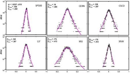
This makes the number of samples for the computation of relative entropies rather sparse and hence the stability and accuracy become questionable. However, if both 𝑅 and 𝑃 can be well fit with 𝑞-Gaussian distributions, analytical expressions for the relative entropies can be derived in terms of the parameters of these distributions. In an earlier work [26] we have shown that the financial market return distributions (S&P 500 and Nasdaq) can be well modelled by 𝑞-Gaussian distributions, even during the dot-com bubble and 2008 crash periods. If the distributions of the returns of individual equities can also be modelled by 𝑞-Gaussians, then we can derive analytical formulas for TRE of an individual equity 𝑃 with respect to the market 𝑅. Figure 2 shows monthly percentage returns of S&P 500 and five randomly chosen individual stocks (both from S&P 500 and Nasdaq) and the corresponding fit to 𝑞-Gaussian distributions. Visual inspection shows that the fits are pretty good. However, to quantify the ‘goodness of fit,’ Kolmogorov-Smirnov (KS) [29] tests are carried out. Briefly, this involves determining the maximum absolute distances Dmax

between the empirical and the synthetic 𝑞-Gaussian cumulative distribution functions (CDF). The fit is good if Dmax is less than a critical distance 𝐃_{𝐜𝐫𝐢𝐭}. The details of constructing synthetic 𝑞

-Gaussian and determining Dmax and 𝐃_{𝐜𝐫𝐢𝐭} are given in [26]. The values of Dmax and 𝐃_{𝐜𝐫𝐢𝐭} for S&P

500 and the five randomly chosen stocks are displayed in Figure 2. In all cases Dmax is < 𝐃_{𝐜𝐫𝐢𝐭}

showing that the distributions of the returns of even the individual stocks can be modelled well with 𝑞-Gaussian distributions.

From equations (9) and (10), the Tsallis 𝑞-Gaussian distributions for the returns of a market index

R and an individual equity P can be written as

𝑅

𝑞

(Ω) =

_𝑍1_𝑞𝑅

[1 + (𝑞 − 1)𝐵

𝑅

(Ω − 𝑀

𝑅

)

2

]

1/(1−𝑞)

(18)

and

8

The normalizations 𝑍_𝑞𝑅 and 𝑍_𝑞𝑃 are given by

𝑍

𝑞𝑅

= 𝐶

𝑞

⁄

√𝐵

𝑅

𝑍

𝑞𝑃

= 𝐶

𝑞

⁄

√𝐵

𝑃

The parameter 𝑞 is estimated from the reference distribution R. All three parameters 𝑞, 𝐵_𝑅 and 𝑀_𝑅 are estimated for R. For P, only 𝐵_𝑃 and 𝑀_𝑃 are estimated using 𝑞 of the reference distribution.

As shown in Appendix A, the Tsallis relative entropy is now given by

𝑆

𝑇

(𝑃ǁ𝑅) = − 𝑙𝑛

𝑞

(𝛾

𝑅𝑃

)

+

1₂

𝛾

𝑅𝑃1−𝑞

[(𝛾

𝑅𝑃2

− 1) + (3 − 𝑞)𝐵

𝑅

(𝑀

𝑃

− 𝑀

𝑅

)

2

]

(20)

Here

𝛾

_𝑅𝑃

= √𝐵

𝑅

𝐵

𝑃

⁄

.

In the limit 𝑞 → 1, 𝑀 → 𝜇

,

𝐵 → 1 (2𝜎⁄ 2),and𝛾_𝑅𝑃→ 𝜎_𝑅𝑃= 𝜎_𝑃⁄𝜎_𝑅 giving the KL relative entropy

𝑆

_𝐾𝐿

(𝑃ǁ𝑅) = − 𝑙𝑛(𝜎

𝑅𝑃

) +

1₂

(𝜎

𝑅𝑃2

− 1) + (𝜇

𝑃

− 𝜇

𝑅

)

2

⁄

(2𝜎

𝑅2

)

(21)

𝑆𝑇(𝑃ǁ𝑅) is evaluated at the estimated parameters 𝑞̂, 𝑀̂ and 𝐵̂. The first two moments are used to

compute the 𝑆_𝐾𝐿.

Note that 𝑆_𝑇 depends non-linearly on the returns since both 𝐵 and 𝑀 have non-linear dependence on the returns (equations (11b) and (11c)). The first two terms in (20) depend only on the generalized standard deviations. The third term is a distance term (complementary to correlation) in generalized average returns. This is a systematic risk as the one addressed in CAPM. Hence Tsallis relative entropy combines aspects of both the standard deviation and CAPM risk measures and addresses the non-linearity of the stock dynamics.

3. Data, Methodology, and Results

3.1 Data

9

years prior to 4 January 2000. This gives us about 365 securities to work with. The data are adjusted for dividends and splits. No attempt has been made to correct the data for inflation.

3.2 Methodology

In testing the performance of the four risk measures in this study (Tsallis relative entropy, Kullback-Leibler relative entropy, relative sigma, and beta), a procedure somewhat similar to that described by Black, Jensen and Scholes [10] is followed. The exact procedure is as follows:

a) Five years of data prior to the starting date 4 January 2000 are used to estimate the parameters of the risk models for the reference market index S&P 500 and for each security. The values of the relative entropy risk measures are calculated from the model parameters. The expected return is computed as the average monthly return (as defined in (1c)) of the security over the next six months (arbitrarily chosen).

b) The risk values are then binned and the securities are assigned to each bin according to their risk value such that there are an equal number of securities in each bin. Note that this makes the bin widths variable. The set of securities in each bin can be considered a portfolio. The risk value of each bin is taken to be the center value of the bin.

c) Assuming an equal amount of money invested in every security, the expected return of the portfolio in each bin in excess of the S&P 500 expected return is calculated. This gives the risk-return values for each portfolio.

The data are then shifted by six months and the procedures a) - c) are repeated. The 𝑞 values, however, are estimated every year. The process is continued until all the data are exhausted. For the data period considered, this gives us 36 samples of average monthly returns for each security.

Note that every time the data are shifted, the contents of each bin in step b) can change. Also, in step c), each bin is rebalanced every six months such that an equal amount of money is invested in every security. This means that if this procedure is applied in practice, some securities would be sold and others bought every six months to implement steps b) and c). The effects on the portfolio returns due to transaction costs incurred in such selling and buying and taxes imposed on realized gains are not included in this study.

Finally, the returns in each bin are further averaged over all the 36 samples of average monthly returns and the bin-risk values are also averaged over all cycles. This gives us the final risk-expected return profile. We denote the risk-expected earnings of the portfolio in excess of risk-expected market return as Erel. Note that the binning procedure is expected to minimize the effect of estimation errors on the performance of the portfolios.

3.3 Goodness of Fit

10

how close the risk-return patterns are to a linear regression. If {s} is a set of risk values of the bins and {e} the corresponding portfolio earnings, then

𝜒

2

= 1 −

∑ [𝑒𝑖 𝑖 − (𝑝0 + 𝑝1𝑠𝑖)]2

∑ (𝑒𝑖 𝑖−𝑒̅)2

(22)

Here 𝑝₀ and 𝑝₁ (intercept and slope) are the parameters of the linear fit and 𝑒̅ is the mean of e. Note that the closer the values of e to the linear fit, the closer is 𝜒2 to 1.

3.4 Results

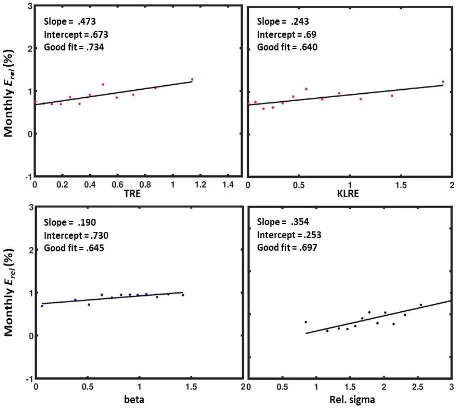
Figure 3 shows the long term behavior of the Erel calculated from monthly returns vs. the risk for the four risk measures considered. The period is 2000-2018. Note that for this long period, the slopes of the linear fit in all four cases are positive, indicating that for greater relative risk there is greater relative return. This behavior is similar to that observed in the tests of the CAPM model [10] as well. However, of all the risk measures, TRE gives the best 𝜒2 (goodness of fit).

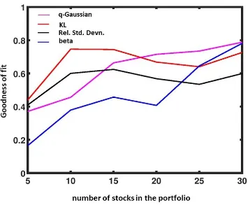
Figure 4 shows the effect of increasing the number of securities in each portfolio (diversification) on the long term performance of the portfolios. In the case of TRE, we observe a consistent behavior of improved performance with an increase in the number of securities in the portfolio. However, this is not the case with the other risk measures. Further, in all cases, the 𝜒2 of TRE is better than that of beta of the CAPM.

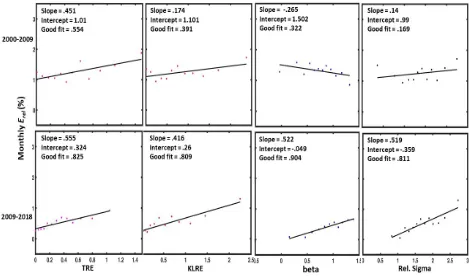
Tests of CAPM by Black, Jensen and Scholes [10] show that for shorter periods (~9 years), even though a linear relationship exists between risk and return, the risk-return patterns are non-stationary, i.e., the slopes and intercepts vary widely for each period, the slopes becoming even negative in some cases. In the present work, we carry out similar tests of the four risk measures, dividing the data into two periods of 9 years each: a) 2000-2009 and b) 2009-2018. Note that the estimation of parameters starts from the data five years earlier: 1995-2004 for a) and 2004-2013 for b). Hence the first interval covers only the dot-com bubble period and the beginning edge of the 2008 crash. As shown in figure 5, the 𝑞 values for period a) varies between 1.24 – 1.45 denoting a relatively calm situation. For interval b) the range is between 1.4 – 1.74 pointing to strong non-extensivity and possibly a chaotic situation. However, the period of 9 years is long enough for the market to reach a calmer period (normal values of 𝑞).

11

Summary and Conclusions

In this work, we have proposed Tsallis relative entropy (TRE) as a novel risk measure for the selection of risk optimal portfolios for returns in excess of market returns. Since the distributions of the returns of both the market (S&P 500) and the individual stocks can be well fit with 𝑞-Gussian distributions, the TRE can be analytically expressed in terms of the model parameters of the 𝑞 -Gaussian distributions. This alleviates several problems (described in 2.3) encountered in the histogram based estimation of relative entropies. Further, the analytical expressions show that TRE has aspects of both the CAPM and the standard deviation risk measures in a non-linear way.

The performance of TRE as a risk measure is compared with those of three other risk measures: KLRE, beta of CAPM, and relative standard deviations. The KLRE is obtained as the limiting 𝑞 → 1 case of TRE.

One of the observations in these empirical tests is the consistent behavior of TRE. First of all, the goodness of fit improves with diversification, which is to be expected. This is not so with the other three measures. The long term behavior is similar in all cases, in the sense that the risk-return profiles show a linear relationship with the linear fit showing a positive slope indicating that the excess returns increase with risk. The goodness of fit for the four risk measures are comparable with TRE showing the best goodness of fit. However, things change in the shorter term behavior. TRE still shows a consistent behavior in terms of good𝜒2values even during shorter intervals covering the dot-com bubble and 2008 crash periods. This is not so for the other three risk measures. This indicates that it might be possible to construct portfolios whose returns can beat the market return even during periods of chaotic behavior, using TRE as the risk measure.

The empirical investigations in this work point to the importance of taking into account the non-linearity and correlations of stock market dynamics in defining risk measures. TRE is one such measure and may help in the construction of portfolios whose returns show a predictive risk-return behavior both in the long and shorter time investments.

This brings us to the question of how short is a ‘shorter time’ to hold the portfolio whose returns

beat the market. That depends on how chaotic the market is and the relaxation time. In the case of Tsallis statistics, one might be able to get a handle on these by estimating 𝑞_{𝑡𝑟𝑖𝑝𝑙𝑒𝑡}[24][30]. This, however, is a subject for future studies.

Acknowledgements

12

Appendix: Derivation of Tsallis q-Gaussian Relative Entropy

Denoting

𝜑 = 1 (𝑞 − 1)

⁄

and

𝜅 = (𝑞 − 1)𝐵

(A1) the integral representation of Tsallis relative entropy (14) is given by

𝑆

𝑇

(𝑃ǁ𝑅) = 𝜑(∫ 𝑃(𝑃 𝑅

⁄ )

1 𝜑⁄

𝑑Ω − 1)

(A2) with the PDF’s 𝑅 and 𝑃 given by

𝑅

𝑞

(Ω) =

_𝑍1_𝑞𝑅

[1 + 𝜅

𝑅

(Ω − 𝑀

𝑅

)

2

]

−φ

(A3)

𝑃

𝑞

(Ω) =

_𝑍1_𝑞𝑃

[1 + 𝜅

𝑃

(Ω − 𝑀

𝑃

)

2

]

−𝜑

(A4)

Here, the normalizations

𝑍

𝑞𝑅

= 𝐶

𝜑

⁄

√𝜅

𝑅

(A5)

𝑍

_𝑞𝑃

= 𝐶

_𝜑

⁄

√𝜅

_𝑃

(A6)

𝐶

𝜑

= √

𝜋

(φ − 1₂₎

(φ )

(A7)

Using (A2) – (A6):

∫ 𝑃 (𝑃 𝑅

⁄ )

1 𝜑⁄

𝑑Ω

= (√𝜅

𝑃

⁄ )

𝜅

𝑅 1 𝜑⁄

(1/𝑍

𝑞𝑃

) ∫

[1+ 𝜅𝑅(Ω−𝑀𝑅)

2_]

[ 1+ 𝜅𝑃(Ω−𝑀𝑃)2]1+ 𝜑

𝑑Ω

=

(√𝜅

_𝑃

⁄ )

𝜅

_𝑅 1 𝜑⁄

(1/𝑍

_𝑞𝑃

) ∫

_{[ 1+ 𝜅}[1+ 𝜅𝑅(𝑀𝑃−𝑀𝑅)2]

𝑃(Ω−𝑀𝑃)2]1+ 𝜑

+

𝜅𝑅(Ω−𝑀𝑃)2

[ 1+ 𝜅𝑃(Ω−𝑀𝑃)2]1+ 𝜑

𝑑Ω

Using:

13

and

∫ 𝜅

𝑅

(Ω − 𝑀

𝑃

)

2

⁄

[1 + 𝜅

𝑃

(Ω − 𝑀

𝑃

)

2

]

1+𝜑

= 𝑍

𝑞𝑃

(

_2𝜑1

)(𝜅

𝑅

⁄ )

𝜅

𝑃

one can write, after some algebra:

𝑆

𝑇

(𝑃ǁ𝑅) = − 𝑙𝑛

𝑞

(𝛾

𝑅𝑃

)

+

1₂

𝛾

𝑅𝑃1−𝑞

[(𝛾

𝑅𝑃2

− 1) + (3 − 𝑞)𝐵

𝑅

(𝑀

𝑃

− 𝑀

𝑅

)

2

]

(A8)

In writing (A8), we have used (A1) and

𝛾

_𝑅𝑃

= √𝐵

𝑅

𝐵

𝑃

⁄

.

References

[1] Sharpe W F, 1964 Capital Asset Prices: A Theory of Market Equilibrium under Conditions of Risk, The Journal of Finance, 19, 425

[2] Fama E F, 1968 Risk, Return and Equilibrium,Report No. 6831 (Chicago; Center for Mathematical Studies in Business and Economics, University of Chicago)

[3] Fama E F, 1968 Risk, Return, and Equilibrium: Some Clarifying Comments, The Journal of Finance, 23, 29

[4] Markowitz H M, 1959 Portfolio Selection: Efficient Diversification of Investments (New York; Wiley)

[5] Jensen M C, 1969 Risk, The Pricing of Capital Assets, and The Evaluation of Investment Portfolios, The Journal of Business, 42, 167

[6] Sharpe W F, 1966 Mutual Fund Performance, The Journal of Business, 39, 119

[7] Fama E F, 1965 The Behavior of Stock-Market Prices, The Journal of Business, 38, 34

[8] Bachelier L, 1964, Theory of Speculation, The Random Character of Stock Market Prices

(Cambridge, MA; MIT Press, ed. Cootner P)

14

[10] Black F, Jensen M C and Scholes M, 1972 The Capital Asset Pricing Model: Some Empirical Tests, Studies in the Theory of Capital Markets (New York; Praeger, ed. Jensen M C)

[11] Clausius R, 1870 On a mechanical theorem applicable to heat, The London, Edinburgh, and Dublin Philosophical Magazine and Journal of Science, 40, 122

[12] Boltzmann L, 2012 Weitere Studien über das Wärmegleichgewicht unter

Gas-molekülen, Wissenschaftliche Abhandlungen Volume 1 (Cambridge: Cambridge University

Press, ed. Hasenöhrl, F)

[13] Shannon C E, 1948 A Mathematical Theory of Communication, The Bell System Technical Journal, 27, 379

[14] Philippatos G C and Wilson C J, 1972 Entropy, market risk, and the selection of efficient portfolios. Applied Economics 4, 209

[15] Dionisio A, Menezes R and Mendes D A, 2006 An econophysics approach to analyse uncertainty in financial markets: an application to the Portuguese stock market, The European Physical Journal B, 50, 161

[16] Maasoumi E and Racine J, 2001 Entropy and predictability of stock market returns,

Journal of Econometrics 107, 291

[17] Zhou R, Cai R and Tong G, 2013, Applications of Entropy in Finance: A Review, Entropy, 15, 4909

[18] Lassance N and Vrins F, 2018 Minimum Rényi Entropy Portfolios, arXiv:1705.05666v4

[19] Ormos M and Zibriczky D, 2002 Entropy-Based Financial Asset Pricing, PLoS ONE 9, 1

[20] Tsallis C, 1998 Generalized entropy-based criterion for consistent testing, Physical Review E 58, 1442

[21] Kullback S, 1959 Information Theory and Statistics (New York, Wiley)

[22] Tsallis C, Anteneodo C, Borland L and Osorio R, 2003 Nonextensive statistical mechanics and economics, Physica A, 324, 89

[23] Osorio R, Borland L and Tsallis C, 2004 Distributions of High-Frequency Stock-Market Observables, Nonextensive Entropy: Interdisciplinary Applications (New York;Oxford University Press, eds. Tsallis C and Gell-Mann M)

15

[25] Mantegna R N and Stanley H E, 2000 An Introduction to Econophysics: Correlations and Complexity in Finance (Cambridge; Cambridge University Press)

[26] Devi S, 2017 Financial market dynamics: superdiffusive or not? Journal of Statistical Mechanics: Theory and Experiment, 2017, 083207

[27] Shalizi C R, 2007 Maximum Likelihood Estimation for q-Exponential (Tsallis) Distributions, arXiv:math/0701854

[28] Furuichi S, Yanagi K and Kuriyama K, 2004 Fundamental properties of Tsallis relative entropy, Journal of Mathematical Physics, 45, 4868

[29] Massey F J, 1951 The Kolmogorov-Smirnov Test for Goodness of Fit, Journal of the American Statistical Association,46, 68

16

Figures

17

[image:18.612.79.530.109.374.2]

18

[image:19.612.77.533.88.497.2]

Figure 3. Average monthly excess returns of the portfolios vs. the four risk measures considered. The reference market index is the S&P 500. Portfolios constructed out of stocks in S&P 500. Number of stocks in each portfolio is 25. Data interval 2000-2018.

19

[image:20.612.130.485.127.420.2]

20

21

[image:22.612.70.539.112.391.2]