Munich Personal RePEc Archive
A New Nonlinear Unit Root Test with
Fourier Function
Güriş, Burak
Istanbul University
October 2017
A New Nonlinear Unit Root Test with Fourier Function
Assoc. Prof. Dr. Burak Güriş
Istanbul University, Faculty of Economics, Istanbul Turkey E-mail: [email protected]
Abstract
Traditional unit root tests display a tendency to be nonstationary in the case of structural breaks and nonlinearity. To eliminate this problem this paper proposes a new flexible Fourier form nonlinear unit root test. This test eliminates this problem to add structural breaks and nonlinearity together to the test procedure. In this test procedure, structural breaks are modeled by means of a Fourier function and nonlinear adjustment is modeled by means of an Exponential Smooth Threshold Autoregressive (ESTAR) model. The simulation results indicate that the proposed unit root test is more powerful than the Kruse (2011) and KSS(2003) tests.
JEL classification: C12, C22
1.Introduction
Almost all of the empirical studies that use the time series techniques use unit root tests. During the last four decades, an increasing number of studies have developed tests to analyze the order of integration of variables. Unit root tests were first introduced to literature by Dickey and Fuller (1979). The change in general in the testing concept was introduced by Perron (1989). According to Perron (1989), traditional unit root tests will display a tendency not to be stationary in the case of a structural break. After Becker et. al. (2006), the flexible Fourier transformation is used quite frequently in modeling structural breaks in recent years. The main advantage of this approach is that it eliminates the need to determine the number and the type of structural breaks.
Enders and Granger (1998) demonstrate that the standard tests for unit root and cointegration all have lower power in the presence of misspecified dynamics. In the light of this information, it is important to determine not only the structural break but also the type of model of the nonlinear structure. There have been significant developments in nonlinear unit root tests in recent years and various significant tests that make use of various types of models have been developed (Kapetanious et al. (2003)(KSS), Sollis (2004, 2009), Kruse (2011)).
Christopoulos and Leon-Ledesma (2010) made a significant contribution to literature by proposing new test procedures that combine Fourier transformation and nonlinearity. This procedure is based upon using the Fourier form in the first stage and the KSS test in the second stage. This allows for modeling both nonlinearity and structural break.
This study proposes a new test procedure combining the Kruse (2011) test developed in the light of the main criticisms to the KSS test with the Fourier transformation. In this test procedure structural breaks are modeled by means of a Fourier function and nonlinear adjustment is modeled by means of an Exponential Smooth Threshold Autoregressive (ESTAR) model as proposed by Kruse (2011).
The proposed unit root test is going to be explained in the second section of the study, the third section is going to focus on the Monte Carlo simulations and measure the critical values, empirical size and the power of the test and the fourth section is going to focus on conclusion.
2. The Flexible Fourier Form Nonlinear Unit Root Test
The recent developments in unit root tests concentrate mostly on using nonlinear model specifications and tests with structural breaks. The structural break tests were first introduced to literature by Perron (1989) and the tests by Zivot and Andrews (1992), Lee and Strazicich (2003, 2004) Carrion-i-Silvestre et al. (2009) were developed later to define the history and the number of structural break tests. Prodan (2008) demonstrate that when the breaks are of opposite sign, it can be difficult to estimate the number and the magnitude of multiple breaks.
Christopoulos and Leon-Ledesma (2010) suggest a unit root test that account jointly for structural breaks and nonlinear adjustment. They modeled structural breaks by means of a Fourier function. They also modeled nonlinear adjustment by means of an ESTAR model proposed by Kapetanious et al. (2003).
This study is an extension of the test proposed by Christopoulos and Leon-Ledesma (2010). The Fourier function was used in the first stage for the proposed test following Christopoulos and Leon-Ledesma (2010) to model structural breaks in unknown forms and numbers. In the second test, the unit root was tested by using the Kruse (2011) test developed in the light of the criticisms made for the KSS test.
The test developed by Kruse (2011) is the advanced version of the root test introduced to literature by Kapetanios et al. (2003). The test developed by Kruse (2011) examines the nonlinear stationary exponential smooth transition autoregressive (ESTAR) against the null hypothesis of unit root.
The ESTAR model could be shown as follows:
2
1 1 1 exp 1
t t t t t
y y y y c
Contrary to Kapetanios et al. (2003), the Kruse (2011) study has shown that in real world examples, the possibility of non-zero location parameter (𝑐 ≠ 0) is imminent (Anoruo and Murthy, 2014). Based on this, the equation was changed as follows using the Taylor approximation in the Kruse (2011) study:
∆𝑦𝑡 = 𝛿1𝑦𝑡−13 + 𝛿2𝑦𝑡−12 + ∑𝑝𝑗=1𝜑𝑗∆𝑦𝑡−𝑗+ 𝜀𝑡
Kruse (2011) proposes a 𝜏 test here to test the null hypothesis of unit root (𝐻0: 𝛿1 = 𝛿2 = 0) against globally stationary ESTAR process (𝐻1: 𝛿1 < 0, 𝛿2 ≠ 0). This test statistics is formulated as follows:
𝜏 = 𝑡𝛿22⊥=0+ 1(𝛿̂1 < 0)𝑡𝛿21=0
Kruse(2011) show that 𝜏 statistic has the following asymptotic distribution which is free of nuisance parameters
𝜏 ⇒ 𝑎(𝑊(𝑟)) + 𝐵(𝑊(𝑟))
The test procedure proposed in the study can be shown as follows similar to the study by Christopoulos and Leon-Ledesma (2010).
Step 1: the nonlinear deterministic component is specified in the first stage.
𝑦𝑡 = 𝛼0+ 𝛼1𝑠𝑖𝑛 (2𝜋𝑘 ∗𝑡
𝑇 ) + 𝛼2𝑐𝑜𝑠 ( 2𝜋𝑘∗𝑡
𝑇 ) + 𝑣𝑡
k* is the optimal frequency and it will be obtained by assigning values to k changing between 1 to 5, then predicting the equation by using OLS and minimizing the total of the squares of error terms. The error terms of the equation predicted will be obtained.
𝑣𝑡 = 𝑦𝑡− 𝛼0− 𝛼1𝑠𝑖𝑛 (2𝜋𝑘 ∗𝑡
𝑇 ) − 𝛼2𝑐𝑜𝑠 ( 2𝜋𝑘∗𝑡
𝑇 )
Step 2: The test statistics is calculated predicting the equation below using the error terms obtained in the first stage:
∆𝑣𝑡= 𝛿1𝑣𝑡−13 + 𝛿2𝑣𝑡−12 + ∑𝑝𝑗=1𝜑𝑗∆𝑣𝑡−𝑗+ 𝜀𝑡
Step 3: If the null hypothesis of unit root is rejected, then
𝐻0: 𝛼1 = 𝛼2 = 0 against the alternative hypotheses 𝐻1: 𝛼1 = 𝛼2 ≠ 0 is tested in this step using the F test. If the null hypothesis is rejected, we can conclude that the variable is stationary around a breaking deterministic function. The critical values of this test are tabulated in Becker
et al. (2006).
3. Monte Carlo Results
The empirical size and power comparison of the critical values for the proposed flexible Fourier form nonlinear unit root test are presented in this section.
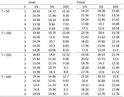
3.1. Critical Values
Table 1: Critical Values for Kruse test with Fourier Aproximation
Level Trend
k 1% 5% 10% 1% 5% 10%
T = 50 1 20.32 14.72 12.32 24.24 18.38 15.66 2 16.04 11.46 9.28 22.34 15.62 13.16 3 14.48 10.14 8.38 19.26 13.96 11.62 4 13.38 9.56 7.92 17.88 13.1 10.88
5 13.58 9.58 7.90 17.5 12.6 10.58
T = 100 1 19.46 14.76 12.44 23.78 18.4 15.78 2 16.06 11.6 9.64 21.42 15.62 13.28 3 14.74 10.7 8.96 18.62 14.46 12.14 4 14.26 10.3 8.64 17.96 13.56 11.58
5 14.26 10.06 8.52 17.8 13.24 11.2
T = 250 1 18.82 14.8 12.52 23.56 18.14 15.74 2 15.84 11.92 9.98 20.02 15.74 13.5 3 15.04 11.14 9.28 18.78 14.2 12.32 4 14.58 10.74 9.1 18.28 13.88 11.96
5 13.98 10.4 8.8 17.76 13.6 11.52
T = 500 1 19.56 14.86 12.7 23.26 18.14 15.8 2 16.36 12.01 9.92 20.4 16.08 13.64 3 14.9 11.24 9.4 19.12 14.6 12.44 4 14.6 10.94 9.2 18.24 13.9 11.98 5 14.34 10.92 9.1 17.66 13.76 11.76
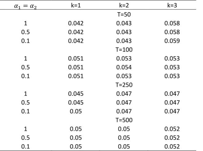
3.2. Finite Sample Size
To evaluate the size of the test statistics, we consider the following data generating process (DGP)
𝑦𝑡 = 𝛼0+ 𝛼1𝑠𝑖𝑛 (2𝜋𝑘𝑇 ) + 𝛼∗𝑡 2𝑐𝑜𝑠 (2𝜋𝑘𝑇 ) + 𝑣∗𝑡 𝑡
𝑣𝑡= 𝑣𝑡−1+ 𝜀𝑡
where 𝜀𝑡 is a sequence of standard normal errors and 𝑘∗ stands for optimal frequency. The empirical size is considered for sample sizes 𝑇 = 50, 100, 250, 500, values of k=1,2,3, and
Table 2 : Empirical Sizes of the Test
𝛼1= 𝛼2 k=1 k=2 k=3
T=50
1 0.042 0.043 0.058
0.5 0.042 0.043 0.058
0.1 0.042 0.043 0.059
T=100
1 0.051 0.053 0.053
0.5 0.051 0.054 0.053
0.1 0.051 0.053 0.053
T=250
1 0.045 0.047 0.047
0.5 0.045 0.047 0.047
0.1 0.05 0.047 0.047
T=500
1 0.05 0.05 0.052
0.5 0.05 0.05 0.052
0.1 0.05 0.05 0.052
The results in Table 2 show that the size of proposed test is close to 5% in all cases with different values of k and 𝛼.
3.3. Empirical Power
We next investigate the power properties of the unit root tests against globally stationary process using the following Fourier-ESTAR model as a DGP:
𝑦𝑡 = 𝛼0+ 𝛼1𝑠𝑖𝑛 (2𝜋𝑘𝑇 ) + 𝛼∗𝑡 2𝑐𝑜𝑠 (2𝜋𝑘𝑇 ) + 𝑣∗𝑡 𝑡
∆𝑣𝑡 = 𝜙𝑣𝑡−1(1 − 𝑒𝑥𝑝{−𝛾(𝑣𝑡−1− 𝑐)2}) + 𝜀𝑡
Table 3 : Power Analysis of Fourier Kruse, Kruse and KSS Tests
T=50 Fourier Kruse Kruse KSS
𝛾 𝑐 k=1 k=2 k=3 k=1 k=2 k=3 k=1 k=2 k=3 0.05 -10 0.94 0.98 0.99 0.83 0.83 0.86 0.88 0.89 0.91 -5 0.6 0.77 0.81 0.44 0.44 0.47 0.49 0.49 0.52 0 0.35 0.55 0.59 0.28 0.27 0.23 0.31 0.31 0.27 5 0.59 0.77 0.81 0.46 0.44 0.47 0.5 0.49 0.52 10 0.94 0.98 0.99 0.84 0.83 0.86 0.9 0.89 0.91 0.1 -10 0.95 0.98 0.99 0.85 0.84 0.87 0.9 0.9 0.92 -5 0.79 0.9 0.93 0.64 0.64 0.68 0.7 0.7 0.75 0 0.58 0.77 0.82 0.44 0.43 0.4 0.47 0.47 0.47 5 0.79 0.9 0.93 0.65 0.65 0.68 0.71 0.72 0.75 10 0.95 0.98 0.99 0.85 0.84 0.87 0.9 0.9 0.92 1 -10 0.95 0.98 0.99 0.85 0.84 0.87 0.89 0.9 0.92 -5 0.95 0.98 0.99 0.84 0.84 0.87 0.9 0.91 0.92 0 0.96 0.99 0.99 0.81 0.81 0.83 0.86 0.86 0.89 5 0.95 0.98 0.99 0.85 0.84 0.87 0.89 0.91 0.92 10 0.95 0.98 0.99 0.84 0.84 0.87 0.9 0.9 0.92
T=100
0.05 -10 0.99 1 0.99 0.99 1 0.99 0.99 1 0.99 -5 0.9 0.94 0.97 0.88 0.89 0.88 0.78 0.79 0.78 0 0.81 0.94 0.96 0.76 0.76 0.75 0.79 0.8 0.79 5 0.89 0.94 0.97 0.87 0.89 0.88 0.79 0.79 0.78 10 0.99 1 0.99 0.99 1 0.99 0.99 1 0.99
0.1 -10 0.99 1 1 0.99 1 1 0.99 1 1
-5 0.98 0.99 0.99 0.97 0.97 0.97 0.95 0.95 0.95 0 0.97 0.99 0.99 0.91 0.92 0.91 0.93 0.94 0.93 5 0.98 0.99 0.99 0.97 0.97 0.97 0.95 0.95 0.95
10 0.99 1 1 0.99 1 1 0.99 1 1
1 -10 0.99 1 1 0.99 1 1 0.99 1 1
-5 0.99 0.99 1 0.99 0.99 1 0.99 0.99 1 0 0.99 1 1 0.99 0.99 0.99 0.99 0.99 1 5 0.99 0.99 1 0.99 0.99 1 0.99 0.99 1 10 0.99 1 1 0.99 1 1 0.99 1 1 Note: T is the sample size.
The results of power experiments are presented in Table 3. A combination of the
4. Conclusion
In this study, a new unit root test which can be useful in the presence of unknown number of breaks and nonlinearity was proposed. The finite sample properties of the suggested test via Monte Carlo simulations were examined. It was found that the proposed test has greater power than the Kruse (2011) and KSS tests. Especially for small sample cases, the power and size performance of the proposed test is good. This test eliminates the problems over-acceptance of the null of nonstationarity to add structural breaks and nonlinearity together into the test procedure.
References
Anoruo, E., & Murthy, V. N. (2014). Testing nonlinear inflation convergence for the Central African Economic and Monetary Community. International Journal of Economics and Financial Issues, 4(1), 1, 1-7.
Becker, R., Enders, W., Hurn., S., (2004). A general test for time dependence in parameters.
Journal of Applied Econometrics 19, 899-906. DOI:10.1002/jae.751
Becker, R., Enders, W., Lee, J., (2006). A stationarity test in the presence of an unknown number of breaks. Journal of time Series Analysis 27, 381-409. DOI:10.1111/j.1467-9892.2006.00478.x
Carrion-i-Silvestre, J. L., Kim, D., & Perron, P. (2009). GLS-based unit root tests with multiple structural breaks under both the null and the alternative hypotheses. Econometric theory, 25(6), 1754-1792. DOI:10.1017/S0266466609990326
Christopoulos, D. K., & León-Ledesma, M. A. (2010). Smooth breaks and non-linear mean reversion: Post-Bretton Woods real exchange rates. Journal of International Money and Finance, 29(6), 1076-1093. DOI: 10.1016/j.jimonfin.2010.02.003
Dickey, D. A., & Fuller, W. A. (1979). Distribution of the estimators for autoregressive time series with a unit root. Journal of the American statistical association, 74(366a), 427-431.
Enders Walter, and Granger C.W.J. (1998). Unit-root tests and asymmetric adjustment with an example using the term structure of interest rates. Journal of Business and Economic Statistics
16(3): 304–311.
Enders, W., & Lee, J., (2012). The flexible form and Dickey-Fuller type unit root tests,
Economics Letters, 117, 196-199. DOI: 10.1016/j.econlet.2012.04.081
Kruse, R. (2011). A new unit root test against ESTAR based on a class of modified statistics. Statistical Papers, 52(1), 71-85. DOI 10.1007/s00362-009-0204-1
Lee, J., & Strazicich, M. C. (2003). Minimum Lagrange multiplier unit root test with two structural breaks. The Review of Economics and Statistics, 85(4), 1082-1089. DOI: 0.1162/003465303772815961
Lee, J., & Strazicich, M. C. (2004). Minimum LM unit root test with one structural break. Manuscript, Department of Economics, Appalachian State University, 1-16.
Perron, P. (1989). The great crash, the oil price shock, and the unit root hypothesis. Econometrica: Journal of the Econometric Society, 1361-1401. DOI: 10.2307/1913712
Prodan, R. (2008). Potential pitfalls in determining multiple structural changes with an application to purchasing power parity. Journal of Business & Economic Statistics, 26(1), 50-65. DOI: 10.1198/073500107000000304
Sollis, R. (2004). Asymmetric adjustment and smooth transitions: a combination of some unit root tests. Journal of time series analysis, 25(3), 409-417. DOI: 10.1111/j.1467-9892.2004.01911.x
Sollis, R. (2009). A simple unit root test against asymmetric STAR nonlinearity with an application to real exchange rates in Nordic countries. Economic modelling, 26(1), 118-125. DOI: 10.1016/j.econmod.2008.06.002
Taylor, M. P., Peel, D. A., & Sarno, L. (2001). Nonlinear Mean‐Reversion in Real Exchange
Rates: Toward a Solution to the Purchasing Power Parity Puzzles. International economic review, 42(4), 1015-1042.. DOI:10.1111/1468-2354.00144
Zivot, E., & Andrews, D. W. K. (2002). Further evidence on the great crash, the oil-price shock, and the unit-root hypothesis. Journal of business & economic statistics, 20(1), 25-44. DOI: 10.1198/073500102753410372