Multi space Variational Encoder Decoders for Semi supervised Labeled Sequence Transduction

Proceedings of the 55th Annual Meeting of the Association for Computational Linguistics, pages 310–320 Vancouver, Canada, July 30 - August 4, 2017. c2017 Association for Computational Linguistics Proceedings of the 55th Annual Meeting of the Association for Computational Linguistics, pages 310–320

Vancouver, Canada, July 30 - August 4, 2017. c2017 Association for Computational Linguistics

Multi-space Variational Encoder-Decoders

for Semi-supervised Labeled Sequence Transduction

Chunting Zhou, Graham Neubig Language Technologies Institute

Carnegie Mellon University ctzhou,[email protected]

Abstract

Labeled sequence transduction is a task of transforming one sequence into another sequence that satisfies desiderata speci-fied by a set of labels. In this paper we proposemulti-space variational encoder-decoders, a new model for labeled se-quence transduction with semi-supervised learning. The generative model can use neural networks to handle both discrete and continuous latent variables to exploit various features of data. Experiments show that our model provides not only a powerful supervised framework but also can effectively take advantage of the

un-labeled data. On the SIGMORPHON

morphological inflection benchmark, our model outperforms single-model state-of-art results by a large margin for the major-ity of languages.1

1 Introduction

This paper proposes a model for labeled sequence transduction tasks, tasks where we are given an input sequence and a set of labels, from which we are expected to generate an output sequence that reflects the content of the input sequence and desiderata specified by the labels. Several exam-ples of these tasks exist in prior work: using labels to moderate politeness in machine translation re-sults (Sennrich et al.,2016), modifying the output language of a machine translation system ( John-son et al., 2016), or controlling the length of a summary in summarization (Kikuchi et al.,2016). In particular, however, we are motivated by the task of morphological reinflection (Cotterell et al., 1_{An implementation of our model are}

avail-able at https://github.com/violet-zct/

MSVED-morph-reinflection.

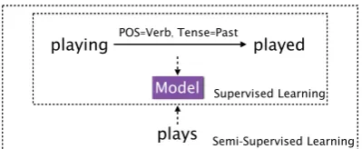
playing POS=Verb, Tense=Past played

Model

plays

SupervisedLearning

Semi-SupervisedLearning

Figure 1: Standard supervised labeled sequence transduction, and our proposed semi-supervised method.

2016), which we will use as an example in our de-scription and test bed for our models.

In morphologically rich languages, different af-fixes (i.e. preaf-fixes, inaf-fixes, sufaf-fixes) can be com-bined with the lemma to reflect various syntac-tic and semansyntac-tic features of a word. The ability to accurately analyze and generate morphologi-cal forms is crucial to creating applications such as machine translation (Chahuneau et al., 2013;

Toutanova et al., 2008) or information retrieval (Darwish and Oard,2007) in these languages. As shown in1,re-inflection of an inflected form given the target linguistic labels is a challenging sub-task of handling morphology as a whole, in which we take as input an inflected form (in the exam-ple, “playing”) and labels representing the desired form (“pos=Verb, tense=Past”) and must

gen-erate the desired form (“played”).

Approaches to this task include those utilizing hand-crafted linguistic rules and heuristics (Taji et al.,2016), as well as learning-based approaches using alignment and extracted transduction rules (Durrett and DeNero,2013;Alegria and Etxeber-ria, 2016;Nicolai et al., 2016). There have also been methods proposed using neural sequence-to-sequence models (Faruqui et al., 2016; Kann et al.,2016;Ostling,2016), and currently ensem-bles of attentional encoder-decoder models (Kann and Sch¨utze, 2016a,b) have achieved state-of-art results on this task. One feature of these neu-ral models however, is that they are trained in a

largely supervised fashion (top of Fig. 1), using data explicitly labeled with the input sequence and labels, along with the output representation. Need-less to say, the ability to obtain this annotated data for many languages is limited. However, we can expect that for most languages we can obtain large amounts of unlabeled surface forms that may al-low for semi-supervised learning over this unla-beled data (entirety of Fig.1).2

In this work, we propose a new frame-work for labeled sequence transduction prob-lems: multi-space variational encoder-decoders (MSVED, §3.3). MSVEDs employ continuous or discrete latent variables belonging to multiple separate probability distributions3 _{to explain the} observed data. In the example of morphological reinflection, we introduce a vector of continuous random variables that represent the lemma of the source and target words, and also one discrete ran-dom variable for each of the labels, which are on the source or the target side.

This model has the advantage of both providing a powerful modeling framework for supervised learning, and allowing for learning in an unsuper-vised setting. For labeled data, we maximize the variational lower bound on the marginal log like-lihood of the data and annotated labels. For un-labeled data, we train an auto-encoder to recon-struct a word conditioned on its lemma and mor-phological labels. While these labels are unavail-able, a set of discrete latent variables are associ-ated with each unlabeled word. Afterwards we can perform posterior inference on these latent vari-ables and maximize the variational lower bound on the marginal log likelihood of data.

Experiments on the SIGMORPHON morpho-logical reinflection task (Cotterell et al.,2016) find that our model beats the state-of-the-art for a sin-gle model in the majority of languages, and is par-ticularly effective in languages with more compli-cated inflectional phenomena. Further, we find that semi-supervised learning allows for signifi-cant further gains. Finally, qualitative evaluation of lemma representations finds that our model is able to learn lemma embeddings that match with human intuition.

2_{Faruqui et al.(2016) have attempted a limited form of} semi-supervised learning by re-ranking with a standard n -gram language model, but this is not integrated with the learn-ing process for the neural model and gains are limited.

3_{Analogous to multi-space hidden Markov models} (Tokuda et al.,2002)

2 Labeled Sequence Transduction

In this section, we first present some notations re-garding labeled sequence transduction problems in general, then describe a particular instantiation for morphological reinflection.

Notation: Labeled sequence transduction prob-lems involve transforming a source sequencex(s) into a target sequence x(t), with some labels describing the particular variety of transforma-tion to be performed. We use discrete variables y₁(t), y₂(t),_{· · ·} , y_K(t) to denote the labels associated with each target sequence, where K is the total number of labels. Lety(t) = [y₁(t), y₂(t),_{· · ·} , y_K(t)]

denote a vector of these discrete variables. Each discrete variabley_k(t) represents a categorical fea-ture pertaining to the target sequence, and has a set of possible labels. In the later sections, we also usey(t)andy_k(t)to denote discrete latent variables corresponding to these labels.

Given a source sequence x(s) and a set of as-sociated target labels y(t), our goal is to gener-ate a target sequence x(t) _{that exhibits the} fea-tures specified byy(t)_{using a probabilistic model} p(x(t)|x(s),y(t)). The best target sequencexˆ(t)is

then given by:

ˆ

x(t)= arg max

x(t)

p(x(t)|x(s),y(t)). (1)

Morphological Reinflection Problem: In mor-phological reinflection, the source sequence x(s) consists of the characters in an inflected word (e.g., “played”), while the associated labels y(t) describe some linguistic features (e.g., ypos(t) =

Verb, y(_tenset) = Past) that we hope to realize

in the target. The target sequence x(t) _is there-fore the characters of the re-inflected form of the source word (e.g., “played”) that satisfy the

lin-guistic features specified by y(t)_{. For this task,} each discrete variabley_k(t)has a set of possible la-bels (e.g. pos=V, pos=ADJ, etc) and follows a

multinomial distribution.

3 Proposed Method

3.1 Preliminaries: Variational Autoencoder

(a) VAE

y(t)

x(t) x(t) _x(s)

x(s) x

x x

z y

z z y z z y(t)

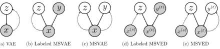
(b) Labeled MSVAE (c) MSVAE (d) Labeled MSVED (e) MSVED

Figure 2: Graphical models of (a) VAE, (b) labeled MSVAE, (c) MSVAE, (d) labeled MSVED, and (e) MSVED. White circles are latent variables and shaded circles are observed variables. Dashed lines indicate the inference process while the solid lines indicate the generative process.

models. We describe it briefly here, and inter-ested readers can refer toDoersch(2016) for de-tails. The VAE learns a generative model of the probabilityp(x_|z) of observed data xgiven a la-tent variable z, and simultaneously uses a recog-nition modelq(z|x)at learning time to estimatez for a particular observationx(Fig.2(a)).q(_·)and

p(_·)are modeled using neural networks parameter-ized byφandθrespectively, and these parameters are learned by maximizing the variational lower bound on the marginal log likelihood of data:

logpθ(x)≥Ez∼qφ(z|x)[logpθ(x|z)]−

KL(qφ(z|x)||p(z)) (2)

The KL-divergence term (a standard feature of variational methods) ensures that the distributions estimated by the recognition model qφ(z|x) do

not deviate far from our prior probabilityp(z) of

the values of the latent variables. To optimize the parameters with gradient descent, Kingma and Welling(2014) introduce a reparameterization trick that allows for training using simple back-propagation w.r.t. the Gaussian latent variablesz. Specifically, we can express z as a deterministic variable z = gφ(,x) where is an independent

Gaussian noise variable ∼ N(0,1). The mean

µand the varianceσ2 ofzare reparameterized by the differentiable functions w.r.t. φ. Thus, instead of generatingzfromqφ(z|x), we sample the

aux-iliary variableand obtainz=µφ(x) +σφ(x)◦,

which enables gradients to backpropagate through φ.

3.2 Multi-space Variational Autoencoders

As an intermediate step to our full model, we next describe a generative model for a single se-quence with both continuous and discrete latent variables, the multi-space variational auto-encoder (MSVAE). MSVAEs are a combination of two threads of previous work: deep generative mod-els with both continuous/discrete latent variables for classification problems (Kingma et al., 2014;

Maaløe et al.,2016) and VAEs with only continu-ous variables for sequential data (Bowman et al.,

2016; Chung et al., 2015; Zhang et al., 2016;

Fabius and van Amersfoort,2014;Bayer and Os-endorfer, 2014). In MSVAEs, we have an ob-served sequence x, continuous latent variables z like the VAE, as well as discrete variablesy.

In the case of the morphology example,xcan be interpreted as an inflected word to be generated.y is a vector representing its linguistic labels, either annotated by an annotator in the observed case, or unannotated in the unobserved case. zis a vector of latent continuous variables, e.g. a latent embed-ding of the lemma that captures all the information aboutxthat is not already represented in labelsy.

MSVAE: Because inflected words can be naturally thought of as “lemma+morphological labels”, to interpret a word, we resort to discrete and continu-ous latent variables that represent the linguistic la-bels and the lemma respectively. In this case when the labels of the sequencey is not observed, we perform inference over possible linguistic labels and these inferred labels are referenced in gener-atingx.

The generative model pθ(x,y,z) =

p(z)pπ(y)pθ(x|y,z)is defined as:

p(z) =N(z|0,I) (3)

pπ(y) = Y

k

Cat(yk|πk) (4)

pθ(x|y,z) =f(x;y,z, θ). (5)

Like the standard VAE, we assume the prior of the latent variable z is a diagonal Gaussian dis-tribution with zero mean and unit variance. We assume that each variable in y is independent, resulting in a factorized distribution in Eq. 4, where Cat(yk|πk) is a multinomial distribution

with parametersπk. For the purposes of this study,

we set these to a uniform distribution πk,j =

1

|πk|. f(x;y,z, θ) calculates the likelihood ofx, a function parametrized by deep neural networks. Specifically, we employ an RNN decoder to gener-ate the target word conditioned on the lemma vari-ablezand linguistic labelsy, detailed in_§5.

When inferring the latent variables from the given data x, we assume the joint distribution of latent variableszandyhas a factorized form, i.e.

The inference model is defined as follows:

qφ(z|x) =N(z|µφ(x),diag(σ2φ(x))) (6)

qφ(y|x) = Y

k

qφ(yk|x)

=Y

k

Cat(yk|πφ(x)) (7)

where the inference distribution overzis a diago-nal Gaussian distribution with mean and variance parameterized by neural networks. The inference model q(y|x) on labels y has the form of a dis-criminative classifier that generates a set of multi-nomial probability vectors πφ(x) over all labels

for each tag yk. We represent each multinomial

distributionq(yk|x)with an MLP.

The MSVAE is trained by maximizing the fol-lowing variational lower boundU(x)on the

objec-tive for unlabeled data:

logpθ(x)≥E(y,z)∼qφ(y,z|x)log

pθ(x,y,z)

qφ(y,z|x)

=Ey∼qφ(y|x)[Ez∼qφ(z|x)[logpθ(x|z,y)]

−KL(qφ(z|x)||p(z)) + logpπ(y)

−logqφ(y|x)] =U(x) (8)

Note that this introduction of discrete variables requires more sophisticated optimization algo-rithms, which we will discuss in§4.1.

Labeled MSVAE: Whenyis observed as shown in Fig. 2(b), we maximize the following varia-tional lower bound on the marginal log likelihood of the data and the labels:

logpθ(x,y)≥Ez∼qφ(z|x)log

pθ(x,y,z)

qφ(z|x)

=

Ez∼qφ(z|x)[logpθ(x|y,z) + logpπ(y)]

−KL(qφ(z|x)||p(z)) (9)

which is a simple extension to Eq.2.

Note that when labels are not observed, the in-ference modelqφ(y|x)has the form of a

discrim-inative classifier, thus we can use observed labels as the supervision signal to learn a better classifier. In this case we also minimize the following cross entropy as the classification loss:

D(x,y) =E(x,y)∼pl(x,y)[−logqφ(y|x)] (10)

wherepl(x,y)is the distribution of labeled data.

This is a form of multi-task learning, as this addi-tional loss also informs the learning of our repre-sentations.

3.3 Multi-space Variational Encoder-Decoders

Finally, we discuss the full proposed method: the multi-space variational encoder-decoder (MSVED), which generates the target x(t) from the sourcex(s)and labelsy(t). Again, we discuss two cases of this model: labels of the target sequence are observed and not observed.

MSVED:The graphical model for the MSVED is given in Fig.2(e). Because the labels of target se-quence are not observed, once again we treat them as discrete latent variables and make inference on the these labels conditioned on the target se-quence. The generative process for the MSVED is very similar to that of the MSVAE with one impor-tant exception: while the standard MSVAE condi-tions the recognition modelq(z_|x)onx, then gen-eratesxitself, the MSVED conditions the recogni-tion modelq(z_|x(s))on the sourcex(s), then gen-erates the targetx(t)_{. Because only the} recogni-tion model is changed, the generative equarecogni-tions for pθ(x(t),y(t),z) are exactly the same as Eqs. 3–5

withx(t) _{swapped forx andy}(t) _{swapped for y.} The variational lower bound on the conditional log likelihood, however, is affected by the recognition model, and thus is computed as:

logpθ(x(t)|x(s))

≥E(y(t)_,z)∼q

φ(y(t),z|x(s),x(t))log

pθ(x(t),y(t),z|x(s))

qφ(y(t),z|x(s),x(t))

=_Ey(t)_∼q

φ(y(t)|x(t))[Ez∼qφ(z|x(s))[logpθ(x

(t)_|y(t)_,z)]

−KL(qφ(z|x(s))||p(z)) + logpπ(y(t))

−logqφ(y(t)|x(t))] =Lu(x(t)|x(s)) (11) Labeled MSVED: When the complete form of x(s),y(t), andx(t)is observed in our training data, the graphical model of the labeled MSVED model is illustrated in Fig.2(d). We maximize the vari-ational lower bound on the conditional log likeli-hood of observingx(t)_andy(t)_{as follows:}

logpθ(x(t),y(t)|x(s))

≥Ez∼qφ(z|x(s))log

pθ(x(t),y(t),z|x(s))

qφ(z|x(s))

=E_z∼q

φ(z|x(s))[logpθ(x

(t)_|y(t)_{,z) + logp}

π(y(t))]−

KL(qφ(z|x(s))||p(z)) =Ll(x(t),y(t)|x(s)) (12) 4 Learning MSVED

useful to its success.

4.1 Learning Discrete Latent Variables

One challenge in training our model is that it is not trivial to perform back-propagation through dis-crete random variables, and thus it is difficult to learn in the models containing discrete tags such as MSVAE or MSVED.4_{To alleviate this problem,} we use the recently proposed Gumbel-Softmax trick (Maddison et al.,2014;Gumbel and Lieblein,

1954) to create a differentiable estimator for cate-gorical variables.

The Gumbel-Max trick (Gumbel and Lieblein,

1954) offers a simple way to draw samples from a categorical distribution with class probabili-tiesπ1, π2,· · · by using the argmaxoperation as follows: one hot(arg max_i[gi + logπi]), where

g1, g2,· · · are i.i.d. samples drawn from the Gum-bel(0,1) distribution.5 _{When making inferences on} the morphological labelsy1, y2,· · ·, the Gumbel-Max trick can be approximated by the continuous softmax function with temperatureτ to generate a sample vectoryˆifor each labeli:

ˆ

yij = P_Nexp((log(_i πij) +gij)/τ)

k=1exp((log(πik) +gik)/τ

(13)

whereNiis the number of classes of labeli. When

τ approaches zero, the generated sample ˆyi

be-comes a one-hot vector. Whenτ >0,ˆyiis smooth

w.r.tπi. In experiments, we start with a relatively

large temperature and decrease it gradually.

4.2 Learning Continuous Latent Variables

MSVED aims at generating the target sequence conditioned on the latent variable z and the tar-get labels y(t). This requires the encoder to generate an informative representation z encod-ing the content of the x(s). However, the varia-tional lower bound in our loss function contains the KL-divergence between the approximate pos-terior qφ(z|x) and the prior p(z), which is

rel-atively easy to learn compared with learning to generate output from a latent representation. We observe that with the vanilla implementation the KL cost quickly decreases to near zero, setting qφ(z|x)equal to standard normal distribution. In

4_{Kingma et al.(2014) solve this problem by} marginaliz-ing over all labels, but this is infeasible in our case where we have an exponential number of label combinations.

5_{The Gumbel (0,1) distribution can be sampled by} first drawing u _∼ Uniform(0,1) and computing g = −log(₋log(u)).

this case, the RNN decoder can easily rely on the true output of last time step during training to de-code the next token, which degenerates into an RNN language model. Hence, the latent variables are ignored by the decoder and cannot encode any useful information. The latent variablezlearns an undesirable distribution that coincides with the im-posed prior distribution but has no contribution to the decoder. To force the decoder to use the latent variables, we take the following two approaches which are similar toBowman et al.(2016).

KL-Divergence Annealing: We add a coefficient λto the KL cost and gradually anneal it from zero to a predefined thresholdλm. At the early stage

of training, we setλto be zero and let the model first figure out how to project the representation of the source sequence to a roughly right point in the space and then regularize it with the KL cost. Although we are not optimizing the tight varia-tional lower bound, the model balances well be-tween generation and regularization. This tech-nique can also be seen in (Koˇcisk`y et al., 2016;

Miao and Blunsom,2016).

Input Dropout in the Decoder: Besides anneal-ing the KL cost, we also randomly drop out the input token with a probability of β at each time step of the decoder during learning. The previous ground-truth token embedding is replaced with a zero vector when dropped. In this way, the RNN decoder could not fully rely on the ground-truth previous token, which ensures that the decoder uses information encoded in the latent variables.

5 Architecture for Morphological Reinflection

Training details: For the morphological reinflec-tion task, our supervised training data consists of sourcex(s), targetx(t), and target tags y(t). We test three variants of our model trained using dif-ferent types of data and difdif-ferent loss functions. First, the single-directional supervised model ( SD-Sup) is purely supervised: it only decodes the target word from the given source word with the loss functionLl(x(t),y(t)|x(s))from Eq.12.

Sec-ond, the bi-directional supervised model ( BD-Sup) is trained in both directions: decoding the target word from the source word and decoding the source word from the target word, which cor-responds to the loss functionLl(x(t),y(t)|x(s)) +

Lu(x(s)|x(t))using Eqs.11–12. Finally, the

maxi-Proposed MSVED Baseline MED

Language #LD #ULD SD-Sup BD-Sup Semi-sup Single Ensemble

Turkish 12,798 29,608 93.25 95.66† 97.25‡ 89.56 95.00 Hungarian 19,200 34,025 97.00 98.54† _99.16‡ _{96.46 98.37}

Spanish 12,799 72,151 88.32 91.50 93.74 94.74†‡ _96.69

Russian 12,798 67,691 75.77 83.07 86.80‡ 83.55† 87.13

Navajo 12,635 6,839 85.00 95.37† _98.25‡ _{63.62 83.00}

Maltese 19,200 46,918 84.83 88.21† 88.46‡ 79.59 84.25

Arabic 12,797 53,791 79.13 92.62† 93.37‡ 72.58 82.80 Georgian 12,795 46,562 89.31 93.63† 95.97‡ 91.06 96.21

German 12,777 56,246 75.55 84.08 90.28‡ 89.11† 92.41

Finnish 12,800 74,687 75.59 85.11 91.20‡ _85.63† _93.18

Avg. Acc – – 84.38 90.78† 93.45‡ 84.59 90.90

Table 1: Results for Task 3 of SIGMORPHON 2016 on Morphology Reinflection. †represents the best single supervised model score,‡represents the best model including semi-supervised models, and bold represents the best score overall. #LD

and#ULDare the number of supervised data and unlabeled words respectively.

k a l b

⌃(x)

µ(x)

✏⇠N(0,1)

z

<w> k

k ä

+

yT

1 y2T y3T y4T.... ...

k a l b

⌃(x)

µ(x)

✏⇠N(0,1)

z

<w> k

k a

Multinomial Sampling

+

...

y12{pos: V, N, ADJ}..

y22{def: DEF, INDEF}

y32{num: DU, SG, PL}...

... ...

Source Word Reinflected Form

Source Word Source Word

Supervised Variational Encoder Decoder

Unsupervised Variational Auto-encoder

y1 y2 y3 y4 · · ·

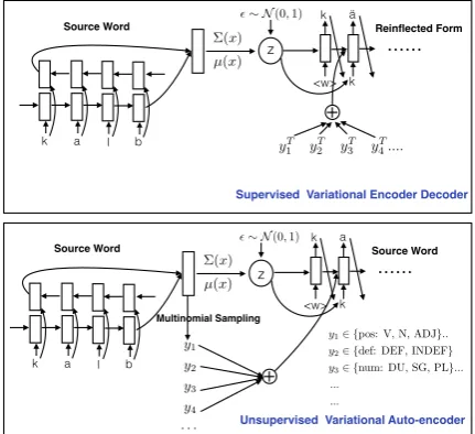
Figure 3: Model architecture for labeled and unlabeled data. For the encoder-decoder model, only one direction from the source to target is given. The classification model is not illus-trated in the diagram.

mize the variational lower bounds and minimize the classification cross-entropy error of10.

L(x(s),x(t),y(t),x) =α· U(x) +Lu(x(s)|x(t))

+_Ll(x(t),y(t)|x(s))− D(x(t),y(t)) (14)

The weightαcontrols the relative weight between the loss from unlabeled data and labeled data.

We use Monte Carlo methods to estimate the expectation over the posterior distributionq(z|x)

and q(y|x) inside the objective function 14.

Specifically, we draw Gumbel noise and Gaussian noise one at a time to compute the latent variables yandz.

The overall model architecture is shown in Fig. 3. Each character and each label is associ-ated with a continuous vector. We employ Gassoci-ated Recurrent Units (GRUs) for the encoder and

de-coder. Let−→htand←h−tdenote the hidden state of the

forward and backward encoder RNN at time step t. uis the hidden representation ofx(s) concate-nating the last hidden state from both directions i.e. [−h→T;h←−T] where T is the word length. u is

used as the input for the inference model onz. We representµ(u) andσ2(u)as MLPs and samplez fromN(µ(u),diag(σ2(u))), usingz=µ+σ◦, where _{∼ N}(0,I). Similarly, we can obtain the

hidden representation ofx(t)_{and use this as input} to the inference model on each labely_i(t)which is also an MLP following a softmax layer to generate the categorical probabilities of target labels.

In decoding, we use 3 types of information in calculating the probability of the next character : (1) the current decoder state, (2) a tag context vec-tor using attention (Bahdanau et al., 2015) over the tag embeddings, and (3) the latent variablez. The intuition behind this design is that we would like the model to constantly consider the lemma represented byz, and also reference the tag cor-responding to the current morpheme being gen-erated at this point. We do not marginalize over the latent variablez however, instead we use the modeµofzas the latent representation forz. We use beam search with a beam size of 8 to perform search over the character vocabulary at each de-coding time step.

Other experimental setups: All hyperparame-ters are tuned on the validation set, and include the following: For KL cost annealing, λm is set

latent variable z to be 150. We setα the weight for the unsupervised loss to be 0.8. We train the model with Adadelta (Zeiler,2012) and use early-stop with a patience of 10.

6 Experiments

6.1 Background: SIGMORPHON 2016

SIGMORPHON 2016 is a shared task on mor-phological inflection over 10 different morpholog-ically rich languages. There are a total of three tasks, the most difficult of which is task 3, which requires the system to output the reinflection of an inflected word.6 _{The training data format in task} 3 is in triples: (source word, target labels, target word). In the test phase, the system is asked to generate the target word given a source word and the target labels. There are a total of three tracks for each task, divided based the amount of super-vised data that can be used to solve the problem, among which track 2 has the strictest limitation of only using data for the corresponding task. As this is an ideal testbed for our method, which can learn from unlabeled data, we choose track 2 and task 3 to test our our model’s ability to exploit this data.

As a baseline, we compare our results with the MED system (Kann and Sch¨utze, 2016a) which achieved state-of-the-art results in the shared task. This system used an encoder-decoder model with attention on the concatenated source word and tar-get labels. Its best result is obtained from an en-semble of five RNN encoder-decoders ( Ensem-ble). To make a fair comparison with our mod-els, which don’t use ensembling, we also calcu-lated single model results (Single).

All models are trained using the labeled training data provided for task 3. For our semi-supervised model (Semi-sup), we also leverage unlabeled data from the training and validation data for tasks 1 and 2 to train variational auto-encoders.

6.2 Results and Analysis

From the results in Tab.1, we can glean a number of observations. First, comparing the results of our fullSemi-supmodel, we can see that for all lan-guages except Spanish, it achieves accuracies bet-ter than the single MED system, often by a large margin. Even compared to the MED ensembled model, our single-model system is quite compet-itive, achieving higher accuracies for Hungarian, 6_{Task 1 is inflection of a lemma word and task 2 is} rein-flection but also provides the source word labels.

Language Prefix Stem Suffix

Turkish 0.21 1.12 98.75 Hungarian 0.00 0.08 99.79 Spanish 0.09 3.25 90.74 Russian 0.66 7.70 85.00 Navajo 77.64 18.38 26.40 Maltese 48.81 11.05 98.74 Arabic 68.52 37.04 88.24 Georgian 4.46 0.41 92.47 German 0.84 3.32 89.19 Finnish 0.02 12.33 96.16

Table 2: Percentage of inflected word forms that have mod-ified each part of the lemma (Cotterell et al., 2016) (some words can be inflected zero or multiple times, thus sums may not add to 100%).

0.2 0.3 0.4 0.5 0.6 0.7 0.8 0.9 1.0

Percentage of suffixing inflection 60

65 70 75 80 85 90 95 100

Accuracy

Navajo _Arabic

Maltese Finnish

Russian Georgian

German Spanish Turkish Hungarian

MSVED MED (1)

Figure 4: Performance on test data w.r.t. the percentage of suffixing inflection. Points with the same x-axis value corre-spond to the same language results.

Navajo, Maltese, and Arabic, as well as achieving average accuracies that are state-of-the-art.

Next, comparing the different varieties of our proposed models, we can see that the semi-supervised model consistently outperforms the bidirectional model for all languages. And simi-larly, the bidirectional model consistently outper-forms the single direction model. From these re-sults, we can conclude that the unlabeled data is beneficial to learn useful latent variables that can be used to decode the corresponding word.

ensem-a l --i m¯a r ¯a t i y y ¯a t u

def=DEF gen=FEM voice=None aspect=None tense=None num=PL poss=None per=None pos=ADJ mood=None case=NOM

n ´ı d a j i d l e e h

arg=None aspect= IPFV/PROG num=PL per=4 pos=V mood=REAL

0.0 0.2 0.4 0.6 0.8

Figure 5: Two examples of attention weights on target lin-guistic labels: Arabic (Left) and Navajo (Right). When a tag equalsNone, it means the word does not have this tag.

bled MED system. To demonstrate this visually, in Fig.4, we compare the semi-supervised MSVED with the MED single model w.r.t. the percentage of suffixing inflection of each language, showing this clear trend.

This strongly demonstrates that our model is ag-nostic to different morphological inflection forms whereas the conventional encoder-decoder with attention on the source input tends to perform bet-ter on suffixing-oriented morphological inflection. We hypothesize that for languages that the inflec-tion mostly comes from suffixing, transducinflec-tion is relatively easy because the source and target words share the same prefix and the decoder can copy the prefix of the source word via attention. However, for languages in which different inflections of a lemma go through different morphological pro-cesses, the inflected word and the target word may differ greatly and thus it is crucial to first analyze the lemma of the inflected word before generat-ing the correspondgenerat-ing the reinflection form based on the target labels. This is precisely what our model does by extracting the lemma representa-tionzlearned by the variational inference model.

6.3 Analysis on Tag Attention

To analyze how the decoder attends to the linguis-tic labels associated with the target word, we ran-domly pick two words from the Arabic and Navajo test set and plot the attention weight in Fig. 5. The Arabic word “al-’im¯ar¯atiyy¯atu” is an adjec-tive which means “Emirati”, and its source word in the test data is “’im¯ar¯atiyyin”7_{. Both of these are} declensions of “’im¯ar¯atiyy”. The source word is

7_{https://en.wiktionary.org/wiki/%D8%}

A5%D9%85%D8%A7%D8%B1%D8%A7%D8%AA%D9%8A

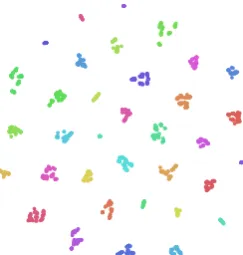
Figure 6: Visualization of latent variableszfor Maltese with 35 pseudo-lemma groups in the figure.

singular, masculine, genitive and indefinite, while the required inflection is plural, feminine, nomi-native and definite. We can see from the left heat map that the attention weights are turned on at sev-eral positions of the word when generating corre-sponding inflections. For example, “al-” in Ara-bic is the definite article that marks definite nouns. The same phenomenon can also be observed in the Navajo example, as well as other languages, but due to space limitation, we don’t provide detailed analysis here.

6.4 Visualization of Latent Lemmas

To investigate the learned latent representations, in this section we visualize the z vectors, ex-amining whether the latent space groups together words with the same lemma. Each sample in SIG-MORPHON 2016 contains source word and tar-get words which share the same lemma. We run a heuristic process to assign pairs of words to groups that likely share a lemma by grouping together word pairs for which at least one of the words in each pair shares a surface form. This process is not error free – errors may occur in the case where multiple lemmas share the same surface form – but in general the groupings will generally reflect lem-mas except in these rare erroneous cases, so we dub each of these groups apseudo-lemma.

In Fig. 6, we randomly pick 1500 words from Maltese and visualize the continuous latent tors of these words. We compute the latent vec-tors asµφ(x)in the variational posterior inference

Language Src Word Tgt Labels Gold Tgt MED Ours

Turkish kocamayaratmamdan pos=N,poss=PSS1S,case=ESS,num=SGpos=N,case=NOM,num=SG kocamdayaratma yaratmakocama yaratmankocamda bitimizde pos=N,tense=PST,per=1,num=SG bittik bitiydik bittim

Maltese ndammhomlitqo˙z˙zhieli pos=V,polar=NEG,tense=PST,num=SGpos=V,polar=NEG,tense=PST,num=SG tindammhiextqo˙z˙zx ndammejthiextqo˙z˙zx tindammhiexqa˙z˙zejtx tissikkmuhomli pos=V,polar=POS,tense=PST,num=PL ssikkmulna tissikkmulna tissikkmulna

Finnish verovapaattaturrumme pos=V,mood=POT,tense=PRS,num=PLpos=ADJ,case=PRT,num=PL turtunemmeverovapaita verovappaitaturtunemme turrunemmeverovapaita sukunimin pos=N,case=PRIV,num=PL sukunimitt sukunimeitta sukunimeitta Table 3: Randomly picked output examples on the test data. Within each block, the first, second and third lines are outputs that ours is correct and MED’s is wrong, ours is wrong and MED’s is correct, both are wrong respectively.

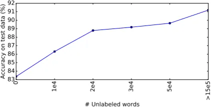
6.5 Analyzing Effects of Size of Unlabeled Data

From Tab. 1, we can see that semi-supervised learning always performs better than supervised learning without unlabeled data. In this section, we investigate to what extent the size of unlabeled data can help with performance. We process a German corpus from a 2017 Wikipedia dump and obtain more than 100,000 German words. These words are ranked in order of occurrence frequency in Wikipedia. The data contains a certain amount of noise since we did not apply any special pro-cessing. We shuffle all unlabeled data from both the Wikipedia and the data provided in the shared task used in previous experiments, and increase the number of unlabeled words used in learning by 10,000 each time, and finally use all the un-labeled data (more than 150,000 words) to train the model. Fig. 7 shows that the performance on the test data improves as the amount of unla-beled data increases, which implies that the un-supervised learning continues to help improve the model’s ability to model the latent lemma repre-sentation even as we scale to a noisy, real, and rela-tively large-scale dataset. Note that the growth rate of the performance grows slower as more data is added, because although the number of unlabeled data is increasing, the model has seen most word patterns in a relatively small vocabulary.

6.6 Case Study on Reinflected Words

In Tab. 3, we examine some model outputs on the test data from the MED system and our model re-spectively. It can be seen that most errors of MED and our models can be ascribed to either over-copy or under-copy of characters. In particular, from the complete outputs we observe that our model tends to be more aggressive in its changes, resulting in

0

1e4 2e4 3e4 5e4

>15e5

# Unlabeled words 83

84 85 86 87 88 89 90 91 92

Accuracy on test data (%)

Figure 7: Performance on the German test data w.r.t. the amount of unlabeled Wikipedia data.

it performing more complicated transformations, both successfully (such as Maltese “ndammhomli” to “tindammhiex”) and unsuccessfully (“tqo˙z˙zx” to “qa˙z˙zejtx”). In contrast, the attentional encoder-decoder model is more conservative in its changes, likely because it is less effective in learning an ab-stracted representation for the lemma, and instead copies characters directly from the input.

7 Conclusion and Future Work

In this work, we propose a multi-space variational encoder-decoder framework for labeled sequence transduction problem. The MSVED performs well in the task of morphological reinflection, outper-forming the state of the art, and further improv-ing with the addition of external unlabeled data. Future work will adapt this framework to other sequence transduction scenarios such as machine translation, dialogue generation, question answer-ing, where continuous and discrete latent variables can be abstracted to guide sequence generation.

Acknowledgments

References

I˜naki Alegria and Izaskun Etxeberria. 2016. Ehu at the sigmorphon 2016 shared task. a simple proposal:

Grapheme-to-phoneme for inflection. In

Proceed-ings of the 2016 Meeting of SIGMORPHON. Dzmitry Bahdanau, Kyunghyun Cho, and Yoshua

Ben-gio. 2015. Neural machine translation by jointly

learning to align and translate. The International

Conference on Learning Representations.

Justin Bayer and Christian Osendorfer. 2014.

Learn-ing stochastic recurrent networks. arXiv preprint

arXiv:1411.7610.

Samuel R Bowman, Luke Vilnis, Oriol Vinyals, An-drew M Dai, Rafal Jozefowicz, and Samy Ben-gio. 2016. Generating sentences from a continuous

space. Proceedings of CoNLL.

Victor Chahuneau, Eva Schlinger, Noah A Smith, and Chris Dyer. 2013. Translating into morphologically rich languages with synthetic phrases. Association for Computational Linguistics.

Junyoung Chung, Kyle Kastner, Laurent Dinh, Kratarth Goel, Aaron C Courville, and Yoshua Bengio. 2015. A recurrent latent variable model for sequential data. In Advances in neural information processing

sys-tems. pages 2980–2988.

R. Cotterell, C. Kirov, J. Sylak-Glassman,

D. Yarowsky, J. Eisner, and M. Hulden. 2016. The sigmorphon 2016 shared taskmorphological

reinflection. In Proceedings of the 54th Annual

Meeting of the Association for Computational Linguistics.

Kareem Darwish and Douglas W Oard. 2007. Adapt-ing morphology for arabic information retrieval. In

Arabic Computational Morphology, Springer, pages 245–262.

Carl Doersch. 2016. Tutorial on variational

autoen-coders.arXiv preprint arXiv:1606.05908.

Greg Durrett and John DeNero. 2013. Supervised learning of complete morphological paradigms. In

Proceedings of the 2013 Conference of the North American Chapter of the Association for Computa-tional Linguistics: Human Language Technologies. Association for Computational Linguistics, Atlanta, Georgia, pages 1185–1195.

Otto Fabius and Joost R van Amersfoort. 2014.

Vari-ational recurrent auto-encoders. arXiv preprint

arXiv:1412.6581.

Manaal Faruqui, Yulia Tsvetkov, Graham Neubig, and Chris Dyer. 2016. Morphological inflection gener-ation using character sequence to sequence

learn-ing. In Proceedings of the 2016 Conference of

the North American Chapter of the Association for Computational Linguistics: Human Language Tech-nologies. Association for Computational Linguis-tics, San Diego, California, pages 634–643.

Emil Julius Gumbel and Julius Lieblein. 1954. Sta-tistical theory of extreme values and some practical

applications: a series of lectures. US Government

Printing Office Washington.

Melvin Johnson, Mike Schuster, Quoc V Le, Maxim Krikun, Yonghui Wu, Zhifeng Chen, Nikhil Thorat, Fernanda Vi´egas, Martin Wattenberg, Greg Corrado, et al. 2016. Google’s multilingual neural machine translation system: Enabling zero-shot translation.

arXiv preprint arXiv:1611.04558.

Katharina Kann, Ryan Cotterell, and Hinrich Sch¨utze. 2016. Neural multi-source morphological

reinflec-tion. arXiv preprint arXiv:1612.06027.

Katharina Kann and Hinrich Sch¨utze. 2016a. Med: The lmu system for the sigmorphon 2016 shared task

on morphological reinflection. In In Proceedings

of the 14th SIGMORPHON Workshop on Computa-tional Research in Phonetics, Phonology, and Mor-phology. Berlin, Germany.

Katharina Kann and Hinrich Sch¨utze. 2016b. Single-model encoder-decoder with explicit morphological

representation for reinflection. InIn Proceedings of

the 54th Annual Meeting of the Association for Com-putational Linguistics. Berlin, Germany.

Yuta Kikuchi, Graham Neubig, Ryohei Sasano, Hiroya Takamura, and Manabu Okumura. 2016. Control-ling output length in neural encoder-decoders. In

Proceedings of the 2016 Conference on Empirical Methods in Natural Language Processing. Associ-ation for ComputAssoci-ational Linguistics, Austin, Texas, pages 1328–1338.

Diederik P Kingma, Shakir Mohamed, Danilo Jimenez Rezende, and Max Welling. 2014. Semi-supervised

learning with deep generative models. In

Ad-vances in Neural Information Processing Systems. Montr´eal, Canada, pages 3581–3589.

D.P. Kingma and M. Welling. 2014. Auto-encoding

variational bayes. InThe International Conference

on Learning Representations.

Tom´aˇs Koˇcisk`y, G´abor Melis, Edward Grefenstette, Chris Dyer, Wang Ling, Phil Blunsom, and Karl Moritz Hermann. 2016. Semantic parsing with

semi-supervised sequential autoencoders. the 2016

Conference on Empirical Methods in Natural Lan-guage Processing (EMNLP).

Lars Maaløe, Casper Kaae Sønderby, Søren Kaae Sønderby, and Ole Winther. 2016. Auxiliary deep

generative models. Proceedings of the 33rd

Interna-tional Conference on Machine Learning.

Chris J Maddison, Daniel Tarlow, and Tom Minka.

2014. A* sampling. In Advances in Neural

Yishu Miao and Phil Blunsom. 2016. Language as a latent variable: Discrete generative models for

sen-tence compression. the 2016 Conference on

Em-pirical Methods in Natural Language Processing (EMNLP).

Garrett Nicolai, Bradley Hauer, Adam St. Arnaud, and Grzegorz Kondrak. 2016. Morphological

reinflec-tion via discriminative string transducreinflec-tion. In

Pro-ceedings of the 2016 Meeting of SIGMORPHON.

Robert Ostling. 2016. Morphological reinflection with

convolutional neural networks. In Proceedings of

the 14th SIGMORPHON Workshop on Computa-tional Research in Phonetics, Phonology, and Mor-phologypage 23.

Rico Sennrich, Barry Haddow, and Alexandra Birch.

2016. Controlling politeness in neural machine

translation via side constraints. In Proceedings of

the 2016 Conference of The North American Chap-ter of the Association for Computational Linguistics (NAACL). pages 35–40.

Dima Taji, Ramy Eskander, Nizar Habash, and Owen Rambow. 2016. The columbia university - new york university abu dhabi sigmorphon 2016

morphologi-cal reinflection shared task submission. In

Proceed-ings of the 2016 Meeting of SIGMORPHON.

Keiichi Tokuda, Takashi Masuko, Noboru Miyazaki, and Takao Kobayashi. 2002. Multi-space

probabil-ity distribution hmm. IEICE TRANSACTIONS on

Information and Systems85(3):455–464.

Kristina Toutanova, Hisami Suzuki, and Achim Ruopp. 2008. Applying morphology generation models to

machine translation. InProceedings of the 46th

An-nual Meeting of the Association for Computational Linguistics. pages 514–522.

Matthew D Zeiler. 2012. Adadelta: an adaptive

learn-ing rate method.arXiv preprint arXiv:1212.5701.

Biao Zhang, Deyi Xiong, Jinsong Su, Hong Duan, and Min Zhang. 2016. Variational neural machine

trans-lation. Proceedings of the 54th Annual Meeting of