Inequality and Well Being

Munich Personal RePEc Archive

Inequality and Well-Being

Borooah, Vani

University of Ulster

May 2018

Online at

https://mpra.ub.uni-muenchen.de/90554/

Chapter 7: Inequality and Well-Being

Abstract

In this chapter, Borooah investigates a neglected area in the study of human development relating

differences in human development between social groups in a country. Failure to take account of such

inter-group inequalities might lead one to exaggerate a country’s developmental achievements.

Conversely, one would get a more accurate picture of a country’s achievements with respect to human

development only after one had taken cognisance of the fact that the fruits of development were

unequally distributed between its various communities. There is a further issue. Not only are

developmental fruits unequally distributed between groups, but these fruits may be unequally

distributed within the groups. In this chapter, Borooah uses the methodology of “equity adjusted

achievement” to compute human development indices and “extended” human development indices

for a number of social groups in India.

7.1. Introduction

The Organisation for Economic Co-operation and Development (OECD) recently observed that

“Concerns have emerged regarding the fact that macro-economic statistics did not portray the right

image of what ordinary people perceived about the state of their lives. Addressing these concerns is

crucial, not just for the credibility and accountability of public services, but for the very functioning of

our democracies” (OECD, 2011, p. 4). Other economists and non-economists have expressed concern

that by identifying welfare exclusively in terms of money income, public policy has lost its way. As a

consequence, there has been — and still is — an undue concentration of both public and private

resources on raising national income: “undue”, because making people richer does not necessarily

improve their well-being or, at any rate, not by enough to justify the outlay of resources in raising

income. In other words, public policy, with its focus on raising national income, may not be giving

people what they want; for this reason, there is a growing restlessness among social scientists about

the wisdom of harnessing economic policy to the yoke of economic performance (Frank, 1997, 1999;

The United Nations, too, recognises that income is not an end in itself but rather a means to

achieving the much broader goal of “human development” and that, towards achieving this goal,

non-economic factors — such as levels of crime, the position of women, respect for human rights etc. —

may, in addition to income, make an important contribution. In order to breathe life into this

perspective, the UNDP regularly publishes, as part of its annual Human Development Report, a

ranking of over 100 countries in terms of their values on the Human Development Index (HDI). This

index, while having GDP performance as one of its components, also takes into account countries’

“achievements” with regard to educational (for example, literacy rates) and health-related (for

example, life expectancy) outcomes.1 “Well-being”, so conceived, may be related to poverty but it is

also quite distinct from it (Subramanian, 2004).

The term “human development” is widely used by the media, politicians, NGOs, and

governments all over the world to mean the capacity of people to fulfil their potential in all the

domains in which they function — inter alia health, education, and income. This concept of

development — based on an expansion of capabilities to function in life, in all its variety and richness

— is arguably a more productive and more expressive view than one based solely on economic

growth. This is a concept which owes much to the work of, among others, Anand and Sen (1994,

1997, 2003), Haq (1994), and Sen (1992). The computation of the Human Development Index, and

the ranking of countries on the basis of their HDI values, have become are regular features of public

debate since the HDI was first published by the United Nations Development Programme (UNDP,

1995, 2000). Another regular feature of HDI is its calculation on a national (and indeed, sub-national

basis), in which different regions of a country are ranked on the basis of their human development (for

example, Shariff, 1999).

Anand and Sen (1994), in a paper prepared for the 1995 Human Development Report, pointed

out that a country’s non-economic achievements were likely to be unequally distributed between

subgroups of its population. For example, in terms of gender equality — which was the focus of their

1

concern — the female literacy rate, or female life expectancy, were often lower than for males. In the

face of such inter-group inequality, they argued that a country’s achievement with respect to a

particular outcome should not be judged exclusively by its mean level of achievement (for example,

by the average literacy rate for a country) but rather by the mean level adjusted to take account of

inter-group differences in achievements. They proposed a method, based on Atkinson’s (1970)

seminal work on the relation between social welfare and inequality, for making such adjustments:

they termed the resulting indicators equity sensitive indicators. This would then allow a comparison

between two countries, one of which had a lower mean achievement level, but a more equitable

distribution of achievement, than the other.They further suggested that assessments of country

achievements should be made on the basis of such equity sensitive indicators rather than, as was often

the case, on the basis of its mean level of achievement.2

A neglected area in the study of human development has been differences in human

development between social groups in a country. So, for example, one might know the value of the

HDI for India in its entirety but fail to adjust this value for the fact that India’s achievements with

respect to the components of the HDI may be unequally distributed between its various social groups:

a national literacy rate may co-exist with high rates of literacy for upper caste Hindus and low rates

for the Scheduled Castes and Scheduled Tribes. Failure to take account of such inter-group

inequalities might lead one to exaggerate India’s developmental achievements. Conversely, one would

get a more accurate picture of India’s achievements with respect to human development only after one

had taken cognisance of the fact that the fruits of development were unequally distributed between its

various communities.

There is, however, a further issue. Not only are developmental fruits unequally distributed

between groups — in the sense that, as observed above, inter-group average incomes may differ —

but these fruits may be unequally distributed within the groups. The former type of inequality is the

domain of inter-group inequality and the latter type of inequality is the domain of within-group

2

inequality with overall inequality being a composite of between- and within-group inequality. So,

pursuing the Anand and Sen (1994, 1997) argument to its logical conclusion, a “proper” assessment of

a country’s achievement with respect to an indicator requires us to take account of inequality not just

in the distribution of that achievement between its social groups but also, within each group,

inequality in the distribution of that achievement between the group’s members.3

The details of the methodology, expressed in mathematical form, which underpins this

concept of “equity-adjusted achievement”, are contained in the following two sections. Then, in

subsequent sections, we use this methodology to compute human development indices and “extended”

human development indices for a number of social groups in India. As is well known, conventional

human development indices embody three elements: education (literacy rate); health (life

expectancy); and income. To this list, we added two further components to arrive at an ‘extended’

HDI: living conditions and social networks. Living conditions are important because many

households in India lack, for example, even basic toilet facilities or ventilation in their cooking area.

Social networks are important because there is a great volume of, admittedly anecdotal, evidence from

India to suggest that it is difficult, if not impossible, to access essential services easily unless one has

personal contacts or, in the vernacular, has jaan-pehchaan.

The results reported in this chapter are based on data from the India Human Development

Survey which relates to the period 2011–12 (hereafter, IHDS-2011).4 This is a nationally

representative, multi-topic panel survey of 42,152 households in 384 districts, 1420 villages and 1042

urban neighbourhoods across India. Each household in the IHDS-2011 was the subject of two

hour-long interviews. These interviews covered inter alia issues of: health, education, employment,

economic status, marriage, fertility, gender relations, and social capital. The IHDS-2011, like its

predecessors for 2005 and 1994, was designed to complement existing Indian surveys by bringing

together a wide range of topics in a single survey. This breadth permits the analysis of associations

across a range of social and economic conditions.

3

These “members” could be households or persons. 4

7.2 Equity Sensitive Achievements

Suppose that there are N households in a country (with measured achievements, X X₁, ₂,...,X_N),

which can be separated into K mutually exclusive social groups (k=1...K ) with Nk households (

1... _k

i= N ) in each group, each household with an achievement, X_ik, 1...i= N_k, 1...k= K. We know

that the average achievement of a country is not achieved by all its groups. Similarly, the average

achievement of a group is not achieved by all its members. In other words, there is inequality in the

distribution of achievements between groups and between individuals in groups. If, as is the

convention in economics, we regard inequality as undesirable (a “bad”) then, in assessing the

achievement of a country or of a group, by how much should we reduce its average achievement to

take account of inequality in achievements?

The answer to this question depends on how averse we are to inequality. In his seminal paper on

income inequality, Atkinson (1970) argued that we (society) would be prepared to accept a reduction

from a higher average income which was unequally distributed to a lower average income which was

equally distributed.5 The size of this reduction would depend upon our degree of “inequality

aversion”, which Atkinson (1970) measured by the value of an “inequality aversion parameter”,ε ≥0.

Whenε =0, we are not at all averse to inequality implying that we would not be prepared to accept

even the smallest reduction in average income in order to secure an equitable distribution. The degree

of inequality aversion increases with the value of

ε

: the higher the value ofε, the more averse we are

to inequality and the greater the reduction in average income we would find acceptable to secure an

equal distribution of income.

These ideas can equally well be applied to the measurement of non-income achievements. We

can reduce the average achievement,

1 N

i i

X X

=

=

∑

, of a country by the amount of inter-group

inequality in achievements to arrive at

X

e, a “group-equity sensitive” achievement for the country:

e

X ≤ X . Similarly, we can reduce the average achievement, X_k, of a group by the amount of

5

group inequality in achievements to arrive at X_ke, a “person-equity sensitive” achievement for the

group: X_ke≤X_k. We refer to

X

e and X_ke as equally distributed equivalent achievements:

X

e, when

it is the achievement of each of the groups (that is, equally distributed between the groups), is welfare

equivalent to

X

; andX_ke, when it is the achievement of every member of group k (that is, equally

distributed between individuals in a group), is welfare equivalent to X_k. The size of these reductions

(as given by the differences:

X

−

X

e andX_k−X_ke) depends upon our aversion to inequality: the

lower our aversion to inequality, the smaller will be the difference; in the extreme case in which there

is no aversion to inequality, there will be no difference between the average, and the equity sensitive,

achievements.

Three special cases, contingent upon the value assumed byε, the inequality aversion

parameter, can be distinguished:

1. ε =0 (no inequality aversion), _Xe _and e k

X are the arithmetic means of, respectively, the group achievements and of the achievements of persons in group k:_Xe _{=X and} e

k k

X =X 2. ε =1, Xe and Xke are the geometric means of, respectively, the group achievements and

of the achievements of persons in group k:

( )

1/ 1 < k K K N e k k

X X X

=

 

=  



∏

 and

1/ 1 k k N N e

k ik k

i

X X X

=

 

=_{ } <



∏

 .

3. ε =2, Xe and Xke are the harmonic means of, respectively, the group achievements and

of achievements of persons in group k:

1 1 K e k k k n X X X − =  

=_{ } <



∑

 and

1 1 1 Nk 1

e k k i k ik X X N X − =  

=_{ } <



∑

 .

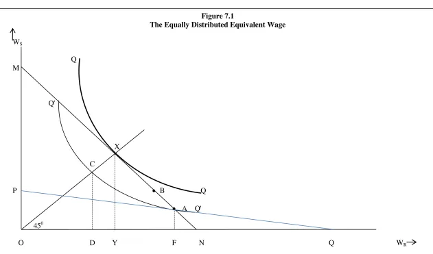
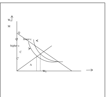
A Diagrammatic Analysis

It may be useful to present the analysis of the preceding paragraphs in diagrammatic terms. Figure 7.1

portrays a world of two persons (R and S) who are required to “share” an achievement, say a given

measures WR and the vertical axis measures WS. The two wages are related to the aggregate wage by

the “sharing” equation: W =(WR+WS) / 2 and this is represented in Figure 7.1 by the “sharing

possibility line”, MN. The point X, on MN, lies on the 450 line passing through the origin and, so, X is

the point at whichWR=WS.

<Figure 7.1>

Given the mean wage, W, the observed distributional outcome may be viewed as a mapping

of W to a point on MN which establishes WR and WS. Different outcomes will locate at different

points of MN. Those that locate closer to the point X (for example, B) will be more egalitarian than

those (like A) which locate further away.

If every person is assigned the same concave utility function U(.), then U W( i)is the utility

that person i (i=R,S) obtains from a wage of Wiand ‘social welfare’, denoted by Q, is defined as the

sum of the utilities of all the children:

( _R) ( _S)

Q U W= +U W

(7.1)

The curves QQ and Q′ Q′ represent indifference curves associated with the welfare function

of equation (7.1), the higher curve (QQ) representing a higher level of utility than the lower curve (Q′

Q′) and these welfare indifference curves are superimposed upon the sharing possibility line.6 Since

the utility functions U(.) in equation (7.1) are assumed to be concave (that is, embodying the property

of diminishing marginal utility), social welfare is maximised when WR =WS that is, when both

receive the same wage.7 Consequently, X is the point at which welfare is maximised and is the point at

which the indifference curve, QQ, is tangential to the sharing possibility line, MN. The distribution,

however, delivers an outcome at point A at which person R receives a higher wage (WR =OF ) and

person S a lower score (WS =AF). The outcome at point A is welfare equivalent to that at point C at

6

An indifference curve shows the different combinations of W WR, S which yield the same level of welfare. It is

obtained by holding Q constant in equation (7.1) and solving for the different W WR, Swhich yield this value of

Q. 7

which both persons receive the same score (WR=WS =CD). CD is then defined as the equally

distributed equivalent (ede) wage.

<Figure 7.2>

The value of the inequality aversion parameter, ε determines the curvature of the indifference

curves. The larger the value of ε, the more ‘bow-shaped’ will be the indifference curve and the

smaller the value of ε, the flatter will be the indifference curve. This is illustrated in Figure 7.2 in

which QQ and W′W′ represent, respectively, indifference curves associated with low and high values

of ε. Both curves pass through the point A on the sharing possibility line MN but CD, the equity

sensitive score associated with QQ (lowε), is greater than C′D′, the ede score associated with Q′Q′

(high ε).

7.3. A Formal Analysis of Equity-Sensitive Indicators

More formally, social welfare, W, is defined as the sum of the concave group utility functions F X( k)

so that:

1

( )

K

k k

k

W N F X

=

=

∑

(7.2)

The change in welfare following a change in theXk is:

1

K

k k k

k

W a N X

=

∆ =

∑

∆ (7.3)

Where: ( k) 0,

k

k

F X a

X ∂

= >

∂ is the marginal change in social welfare consequent upon changes in group

achievements (∆X_k) and also termed the “welfare weight” associated with group k. Since it is

assumed that the functions F(.) are strictly concave, marginal gain decreases with increasing

achievements: consequently, social welfare is maximised when achievements are equal across groups

: X₁=X₂= =... X_K.

The social welfare function, W, in equation (7.2) has constant elasticity if, for ε>0, F(.) can be

1 ₁

( ) , 1, 0; ( ) log( ), 1

1

k

k k k

X

F X F X X

ε

ε ε α β ε

ε

− ₋

= ≠ > = + =

− (7.4)

since then: ( k) ( )1 k k (1 ) k

k k

k k k k

F X a X X

a X X

X X a X

ε ε ε ε ε − − + − ∂ ∂ = = ⇒ = − = −

∂ ∂ . Consequently, the percentage

change in the welfare weight, ak, associated with group k, following an increase in its achievement,

k

X , is constant and negative. The larger the value of the parameterε >0, the greater will be the fall

in the welfare weight.

Similarly, the social welfare of a group W k_k, =1...K is defined as the sum of the concave

utility functions of the group’s members, F X( _k) so that:

1 ( ) k N k ik i

W F X

=

=

∑

(7.5)

Implying:

1

K N

k ik ik

i

W a X

=

∆ =

∑

∆ where the welfare weights, a_ik are defined as: ( ik) 0

ik ik F X a X ∂ = > ∂ .

The social welfare function, Wk, in equation (7.4) has constant elasticity if, for ε>0, F(.) can

be written as:

1 1

( ) , 1, 0; ( ) log( ), 1

1

ik

ik ik ik

X

F X F X X

ε

ε ε α β ε

ε

− ₋

= ≠ > = + =

− (7.6)

Since Xe is welfare equivalent to X and since Xke is welfare equivalent to e k

X we have

Atkinson’s inequality index, I, derived as8:

1/1

1/1 ₁

1

1 1

1

1 1 and 1 1

k

e N

e K

k k ik

k k

k k k i k

X X X

X

I n I

X X X N X

ε

ε _ε

ε − − −

− = =     _{   }     _{ } = −_{ }= − _{ }  = −_{ }= − _{ }      

  _

∑

_   _

∑

  _ (7.7)

where, in equation (7.7), I represents the overall index and Ik represents the inequality index for group

k.

From equation (7.7):

8

Since, by welfare equivalence ofXe and X

1 1 1 1 1

1 1 1

1/1

1 1 1

1 1

( ) ( ) ( ) 1 ( 1) ( ) . Dividing both sides by ,

1 1

K K K

e e e

k k k k k k

k k k

e K e K

k k

k k

k k

NF X N F X X n X X n X X

X X

X X

n n

X X X X

ε ε ε ε ε

ε

ε ε ε

1 1 1 1

1 1

1

( ) ( ) and ( )

k k

N N

e e

k k k ik

k i k

X n X X X

N

ε ε ε ε

− − − −

= =

=

∑

=

∑

(7.8)

From equation (7.8):

( )

( )

( )

(

)

1 2 1 1 1

1 1 1

1 2

1 2

1 1 1 2 1

1 1 1 1

1 1 2 2

1 1

( )

1 1 1

.. ( ) ( ) ... ( ) ( ) K N e ik i

N N N

K

i i iK

i i i K

K

e e e e

K K k k

k

X X

N

N N N

X X X

N N N N N N

n X n X n X n X

ε ε

ε ε ε

ε ε ε ε

− − = − − − = = = − − − − = = = + + + = + + + =

∑

∑

∑

∑

∑

(7.9)

Equation (7.9) represents what Anand and Sen (1994) refer to as “(1-ε) averaging)”: the

overall equally distributed equivalent achievement,

X

eis a weighted average, with exponent 1−ε, of

the group equally distributed equivalent achievements,X_ke (k=1... )K .

A special case occurs when

ε

=0 (no inequality aversion). In that situation,

X

e and X_ke

are the arithmetic means of, respectively, the group achievements and of the achievements of persons

in group k:

X

e

=

X

andX_ke =X_k. When

ε

>0 (there is positive inequality aversion),

X

e

<

X

and

e

k k

X <X .

The Welfare Effects of Redistribution

To examine the welfare effects of an inter-group redistribution of achievements, consider two social

groups — Hindus (k=C) and Muslims (k=D) —and suppose that, within the context of a fixed overall

achievementX , there is a redistribution of achievements (say, income) from Hindus towards Muslims. Then this implies that

0 ( / ) , : 0, 0

C C D D C C D D D C D

X n X n X X n n X θ X where X X

∆ = ∆ + ∆ = ⇒ −∆ = = ∆ ∆ < ∆ > (7.10)

The change in social welfare that results from this redistribution is:

( C) ( D)

C C D D C C C D D D

C D

C C C D D D

F X F X

W N X N X a N X a N X

X X

X−εN X X−εN X

∂ ∂

∆ = ∆ + ∆ = ∆ + ∆

∂ ∂

= ∆ + ∆

(7.11)

C C

C D C D

D D

X N

X X X X

X N

ε

ε

λ θ

−

   

∆ = ∆ ⇒ ∆ = ∆

   

    (7.12)

where: C 1 and = D

D C

X N

X N

λ= > θ .

Suppose that through appropriate redistribution policies, the achievement (income) of

Muslims is increased by one unit. If ε =0, from equation (7.11), in order to keep the overall

achievement,X , unchanged, the achievement (income) of Hindus must fall by ∆X_C =θ. If the fall in the achievement of Hindus exceeded θ, then that would lower the overall achievement X and,

therefore, overall welfare, W.

Since, if ε >0 ∆X_C =λ θ θε > , the achievement of upper-caste Hindus can fall by more than θ — the amount required to keep X unchanged — and still keep welfare unchanged. In other words,

forε >0, society would be prepared to tolerate a fall in the overall achievement (∆ <X 0) in order to

redistribute from Hindus to Muslims, leaving overall welfare unchanged. The greater the value ofε,

the greater will be this tolerance.

6.4 The Equity --Sensitive Human Development Index: Theory

Given a list of M achievement indicators (indexed, j=1…M) — hereafter referred to as, simply,

“indicators” — a country’s performance index (PI) with respect to indicator j, Aj, is defined as

{ }

100

{ } { }

j j

j

j j

X Min X A

Max X Min X −

= ×

− (7.13)

Where A_j is the PI of a countryin respect of achievement j (j=1,2,.., M), X_jis the value of indicator j

and Max X{ _j}and Min X{ _j}are, respectively, the maximum and minimum values of the indicator.

Equation (7.13) implies that 0≤A_j≤100, 1...j= M so that Aj represents the percentage

performance of the country with respect to the jth indicator. The overall performance of the countryis

then the value of its Human Development Index (HDI) and this is defined as the average of the M

1 1 M j j HDI A M =

=

∑

(7.14)

This section applies the idea of the HDI to a situation where the population of a country is

subdivided into K mutually exclusive groups indexed k=1…K. For every household in each group,

we compute the value of its PI in respect of M indicators where these are represented by

, 1... ; 1.... ; and 1...

jkh k

A j= M k= K h= H , where Hk is the number of households in group k. So, for

any group k (k=1…K) and indicator j(j=1…M), the components of the vector

1 2

( , ,... )

k

j k jk j kH

A A A

=

jk

A represents the distribution of the PI with respect to indicator j over the Hk

households in group k. We can then define by Aejk the equally distributed equivalent performance

index, or EDEPI,of group k with respect to indicator j as the (1-ε) average — as defined in equation

(7.9) — of the PI of the groups’ households:

1 1 1 1 ( ) ( ) k H e jk jkh h k A A H ε ε − − =

=

∑

(7.15)

When ε=0, Ae_jk is the arithmetic mean of the household PI; when ε >0, e jk

A is less than the

arithmetic mean of the households’ PI.

The overall EDEPI for group k,k=1…K is:

1 2

1 1 1

...

e e e e

k k k Mk

A A A A

M M M

= + + + (7.16)

The EDEPI aggregated over all the households in all the groups, with respect to attainment j,

and taking account of both within and between group inequalities, is denoted

A

e_j where:

( )

1

( )

1

1 1 1 K Hk

e e j jkh k h A A H ε ε − − = =

=

∑∑

(7.17)

where: 1 K k k H H =

=

∑

is the total number of households in the country.

(

1 2

)

1

...

e e e e

M

A A A A

M

= + + + (7.18)

The Decomposition of the Human Development Index

Setting ε=0 in equation (7.17) and using equation (7.15) yields:

1 1 1 1 1 1

1 K Hk 1 K Hk k 1 Hk k

e e k e k e k e

i ikh ikh ikh ik

k h k k h k k h k

H H H

A A A A A

H = = H = H = = H H = = H

=

∑∑

=

∑ ∑

=

∑

∑

=

∑

(7.19)

If within-group inequalities are ignored then, in each group, every household is assumed to

have the mean PI of that group:Ajhk =Ajk , h=1…Hk, (for i=1…M and k=1,…K). The only inequality

is between group inequality resulting from the fact that the mean PI of the groups, with respect to

indicator j, are different: A_j1≠ A_j2≠....≠A_jK The equally distributed equivalent performance

indicator (EDEPI), aggregated over all the groups, with respect to attainment i, taking account of

between group inequalities only, is denoted

B

e_jwhere:

( )

1

( )

1

1

K e

j k jk

k

B n A

ε

ε −

−

=

=

∑

(7.20)

where: nkis the proportion of households in group k, k=1..K. Then:

The overall EDEPI over all the households in all groups, taking account of only inter-group

inequality is:

1 1 M e e j j B B M =

=

∑

(7.21)

When ε=0, so that there is no aversion to between-group inequality, Bej =Bjwhere

1

K

j k jk

k

B n A

=

=

∑

is the mean of the PI of the indicator j computed over households in all the groups. In

this case, equation (7.21) becomes:

1 1 M j j B B M =

which is, in fact, the HDI defined in equation (7.14). The B in equation (7.22) or, equivalently, the

HDI in equation (7.14) is a special case of _Ae_{in equation (7.18) and obtains when both inter- and}

intra-group inequality in the distribution of the PI between the households in the country is ignored.

6.5 The Human Development Index: Practicalities

In practical terms, the Human Development Index (HDI) has been formulated in terms of a country’s

shortfall in respect of three “dimensions”: living standards, education, and health. Suppose that X, Y,

and Z are the values of a country’s performance indices with respect to each of these three dimensions

and suppose that Max(X), Max(Y), and Max(Z) are the maximum — and Min(X), Min(Y), and Min(Z)

are the minimum — values of these achievements. For example, per-capita gross domestic product

(GDP) is used as a surrogate for living standards with the assumption, say, that Max(X)=$40,000 and

Min(Z)=$100; if Y, the literacy rate in a country, is used as a surrogate for the education dimension

then Max(Y)=100 and Min(Y)=0; if Z, the life expectancy at birth is used as a surrogate for the health

dimension then (it is assumed) Max(Z)=85 and Min(Z)=25.

Following from this, the index for each achievement is defined as: –

10

– 0

Observed value Minimum value Performance Index

Maximum value Minimum value×

=

and the HDI is defined as:

3

X Y Z

Index Index Index

HDI = + +

Now suppose that there are two groups. If we consider the performance index (PI) with

respect to income,9 households within each group will have different PI values and this will yield the

group’s average PI value: suppose X₁ represents group 1’s average PI value andX₂ represents group 2’s average PI value.10 The PI value for each group represents the average distance between its actual

income and its potential income: so, for example, PI=65 for a group means that, on average, it fulfils

65% of its income potential.

One can compute, for each group, its equally distributed equivalent performance index

(EDEPI) with respect to income by taking account of income inequality between the households in the

9

That is,

income

Observed Income Minimum Income Index

Maximum Income Minimum Income

=

−

10

groups: these are denotedX₁e and X₂e. By definition: X₁e ≤X₁ and X₂e ≤X₂ with equality holding if, and only if, there was no aversion to inequality (ε=0) in computing the EDEPI for income. As shown

in the previous section, theX₁e and X₂e are calculated through a process of “ (1−ε)averaging”,

described in equations (6.9) and (6.15). In addition to computing_Xe_{, we can also compute the EDEPI}

for education (the literacy rate) for groups 1 and 2 as,Y₁e and Y₂eand the EDEPI for health (life

expectancy) as Z₁e and Z₂e, and having done so, contrast them with their corresponding average

values, X X Y Y Z₁, ₂, ,_{1 2}, ₁, and Z₂.

Following from this, one can compute the conventional and equity sensitive HDI for each group k

(k=1,2) — respectively, HDI_kavg and HDI_keqs — as:

and

3 3

e e e

avg k k k eqs k k k

k k

X Y Z X Y Z

HDI = + + HDI = + +

This is equation (7.15), above.

After this, the EDE index values for the country can be computed, with respect to each of the

three achievements, by aggregating across the groups. Doing so takes account of inequality in the

distribution of the values of income over all the households in the country: in other words, both

inequality between groups and inequality within groups are taken into account in computing the

country’s EDEPI with respect to income. This is represented byXe where Xe ≤X and the gap

betweenXe and X , the average achievement value for the country, depends upon our aversion to

inequality (in the extreme case, when there is no aversion to inequality, Xe =X ). Similarly, we

compute Ye (EDEPI for the literacy rate) and Ze(EDEPI for life expectancy).11

Following from this, one can compute the conventional and equity sensitive HDI for the

country — respectively, HDIavg and HDIeqs— as:

and

3 3

e e e

avg X Y Z eqs X Y Z

HDI = + + HDI = + +

This is equation (7.18).

11

Alternatively, one could ignore within group inequality by assuming that every household in a

group earns that group’s average income. On this assumption, the country’s EDE achievement with

respect to the income index is represented as e B

X where e

B

X ≤X and the gap betweenX_Be and X, the

average achievement value, depends upon our aversion to inequality (in the extreme case, when there

is no aversion to inequality, X_Be =X). Following from this, the conventional and equity sensitive

HDI for the country, respectively, HDIavg and HDIBeqs, only taking account of between group

inequality, are computed as, by equation (7.20):

and

3 3

e e e

avg eqs B B B

B

X Y Z

X Y Z

HDI = + + HDI = + +

6.6. Data and Analysis: the component indices

The data for the analysis were provided by the household file of the IHDS-2011 which contained

information, pertaining to 2011, on over 42,000 households in India. Using these data, the households

were divided into the following mutually exclusive groups: Scheduled Tribe (ST), Scheduled Caste

(SC), non-Muslim Other Backward Classes (NMOBC), Muslims, non-Muslim Upper Classes

(NMUC). These comprised, respectively, 8.2%, 21.8%, 35.9%, 11.4% and 22.7% of the sample of

households.12

The conventional HDI has, as discussed in the previous section, three dimensions: living

standards (with GDP as the surrogate), education (with the literacy rate as the surrogate), and health

(with life expectancy as the surrogate). Since the analysis reported in this chapter builds up the HDI

from the level of the household, taking account of inter- and intra-group inequality, it uses surrogates

at the household, rather than at the national, level: household per-capita consumption expenditure

(PCE) for living standards and the highest level of education, measured by years of education, of

household adult(s) for education.13 So as to eliminate extreme values, the maximum and minimum

12

All figures reported in this chapter were obtained after grossing up the sample using the household weights provided in IHDS-2011.

13

values of household PCE were taken as the mean values for households in the 95th and 5th quintile of

PCE: these were, respectively, ₹68,195 and ₹7,368.

In order to capture more fully the well-being of households, and of the social groups to which

they belonged, two further dimensions were added. The first of these was the households’ living

conditions. The IHDS-2011 reported on the living conditions of the households with respect to a

number of items from which this study chose seven, scoring as 1 if the household possessed that item

and 0 if it did not: (i) a toilet in their dwelling; (ii) a separate kitchen; (iii) a vent in the cooking place;

(iv) a pucca roof; (v) a pucca floor; (vi) electricity; (vii) water supply in the dwelling or its

compound.14 Thus the maximum and minimum scores score for a household were 7 (it possessed all

seven items) and 0 (it possessed none of these items) and the PI for a household, with respect to living

conditions, was: [observed score/7]×100.

Nearly 83% of households had electricity; the next most commonly possessed housing

amenity (73% of households) was a vent in the cooking area; this was followed by a pucca roof and

floor (respectively, 64% and 59% of households); the least common amenities were a toilet (53% of

households), a separate kitchen (55% of households), and water supply within the precincts of the

dwelling (51% of households).

The second additional dimension was social networks. These are important because there is

evidence (Bros-Bobbin and Borooah, 2013) that it is difficult in India, if not impossible, to easily

access public services unless one ‘knows someone’ or, in the vernacular, has jaan-pehchaan.15 The

IHDS-2011 reported on the social networks of each household with respect to a number of indicators

designed to measure the range, quality, and the closeness of social contacts. The basic questions were:

(i) do you know a person of type X as part of your relatives/caste/community? (ii) If the answer to (i)

is no, do you know a person of type X outside your relatives/caste/community? Type X was

represented by five professions: (a) doctor; (b) principal/teacher; (c) government officer; (d) elected

politician; (e) police inspector.

14

The roof and floor could be: ‘kutcha’ (grass, mud, thatch, wood, tile, slate for the roof; mud or wood for the floor); or ‘pucca’ (asbestos, metal, brick, stone, concrete for the roof; brick, stone, cement, tiles for the floor). 15

In this study, a positive answer by a household to question (i) was scored as 2; a positive

answer to question (ii) was scored as 1; and a score of 0 was assigned to any household that did not

know any type X person whether from within its relatives/caste/community or outside. Consequently,

the maximum and minimum scores for a household with respect to social networks were 5 (a

household knew all five types of persons — doctor, teacher, government officer, elected politician,

police inspector — as part of its relatives/caste/community) and 0 (a household did not know any of

these five types whether as part of, or outside, its relatives/caste/community: the PI for a household,

with respect to social networks was, therefore, [observed score/5]×100.

The IHDS-2011 showed that the two professions with which households were most

acquainted were doctors and teachers: of the sampled households, 20% and 31% knew a doctor and a

teacher, respectively, as part of their relatives/caste/community. This acquaintance was unevenly

distributed between the social groups: 31% of NMUC households — compared to only 12% of ST

households, 15% of SC households, 17% of NMOBC households, and 25% of Muslim households —

knew a doctor, while 44% of NMUC — compared to only 28% of ST households, 24% of SC

households, 27% of NMOBC households, and 32% of Muslim households — knew a

teacher/principal.

The least known types were government officers, elected politicians, and police inspectors:

only 9%, 9%, and 6%, respectively, knew persons of these types as part of their

relatives/caste/community. Of households knowing a government officer, 42% and 28% belonged to

respectively, the NMUC and to the NMOBC; of households knowing an elected politician, 35% and

29% belonged to respectively, the NMUC and to the NMOBC; of households knowing a police

inspector, 36% and 30% belonged to respectively, the NMUC and to the NMOBC. Thus, while not

many households could claim to know government officers, elected politicians, or police inspectors as

part of their relatives/caste/community, those that could were drawn overwhelmingly from the ranks

of the NMUC and the NMOBC.

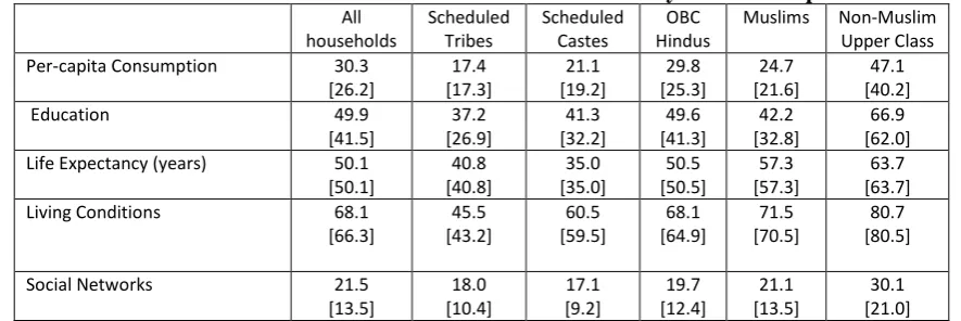
<Table7.1>

Table 7.1 shows the PI values of each group with respect to the five dimensions of the HDI:

in each column is the mean value for each group: this does not adjust for within-group inequality in

the distribution of household PI or, in other words, is based on zero aversion to inequality. In terms of

the algebra, this number is derived from equation (7.15) with ε=0. The number immediately below

this, enclosed in [ ] in Table 7.1, represents the equally distributed equivalent performance index

(EDEPI): the mean values reported are adjusted downwards to take account of inter-household

inequality within each group. In terms of the algebra, this number is derived from equation (7.15) with

ε=0.5, that is with mild inequality aversion.

Table 7.1 shows that, for every dimension, households from the NMUC had the highest,

while households from the Scheduled Tribes and the Scheduled Castes had the lowest, PI values.

Taking account of inter-household inequality reduced the PI below its mean value. These falls were

most marked for the SC and Muslims in terms of education and social networks. The SC have their

privileged sub-castes whereby the benefits of reservation in terms of jobs and education are captured

by a “creamy layer”.16 Muslims, too, have their own privileged groups. The Sachar Committee Report

(2006) refers to the caste system applying also to Muslims: Muslims who were converts to Islam from

the higher casteswere ashraf (meaning “noble”) and regarded as high-born Muslims, while converts

to Islam from the lower castes were ajlaf (meaning “degraded” or “unholy”). As Trivedi et al. (2016)

report, there is little social interaction between the two Muslim “castes”. The existence of privileged

subgroups among deprived groups implies that when allowance is made for intra-group inequality, the

values of EDEPI for deprived groups are considerably lower than their corresponding mean values.

The SC and Muslims are not only deprived but their deprivation is also compounded by the fact that

their attainments are unfairly skewed in favour of a privileged few among them.

Aggregation over Social Groups

In order to obtain the group achievements in respect of the dimensions — living standards, education,

life expectancy, living conditions, and social networks — one needs to aggregate over all the

households in each group, using the method of “1-ε averaging” of equation (7.15), in order to obtain

16

the values of performance index of each group (shown in Table 7.1) in respect of that component. If

the performance index of group k (k=1…) with respect to living standards, education, life expectancy, living conditions, and social networks are represented by, respectively, PILSk, PIEDk, PILEk, PILCk,

and PISNk , then from equation (7.17), the Human Development Index (HDIk) of each group k, over

the five dimensions, is defined as:

0 0 0 0 0 0

0.5 0.5 0.5 0.5 0.5 0.5

1

5 5 No inequality aversion ( 0)

5 1

5 5 Mild inequality aversion ( 0.5)

5

k k k k k k

k k k k k k

HDI PILS PIED PILE PILC PISN

HDI PILS PIED PILE PILC PISN

ε ε ε ε ε ε

ε ε ε ε ε ε

ε

ε

= = = = = =

= = = = = =

 

= _ + + + + _ =

 

= _ + + + + _ =

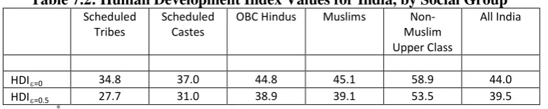
These HDI values are shown in Table 7.2. If one interprets a group’s HDI value as the

percentage fulfilment of its “potential”, then the numbers in Table 7.2 show that, in terms of overall

human development, households in the NMUC collectively fulfilled 58.9% of their potential when

intra-household inequality was ignored and 53.5% of their potential when intra-household inequality

was taken into account. In contrast, Muslims and NMOBC households fulfilled around 45% of their

potential when household inequality was ignored and 39% of their potential when

intra-household inequality was taken into account. Bringing up the rear, ST and SC intra-households fulfilled

around 35% of their potential when intra-household inequality was ignored and around 30% of their

potential when intra-household inequality was taken into account.

<Table 7.2>

The all-India performance index values for each of the five indicators were shown in Table

7.1, under the column labelled all households, both when intra-household inequality (over all the households in India) was ignored (ε=0) and when it was taken into account(ε=0.5). Using these

values, equation (7.18) defines the all-India HDI as:

0 0 0 0 0 0

0.5 0.5 0.5 0.5 0.5 0.5

1 5 1 5

HDI PILS PIED PILE PILC PISN

HDI PILS PIED PILE PILC PISN

ε ε ε ε ε ε

ε ε ε ε ε ε

= = = = = =

= = = = = =

 

= _ + + + + _

 

= _ + + + + _

7.7 Explaining Intra-Household Variation in Performance Indices

The analysis of the preceding sections highlighted the fact that the performance indices (PI) were

unequally distributed between households. The components of the vector A_j=(A_1j,A_2j,...A_Nj)

represent the distribution of the PI with respect to indicator j over the N households (indexed, i=1…N)

in the sample. In the preceding analysis, the sample was divided into five social groups and

differences between them, in the average value of their performance indices for each of five

indicators, were examined.

These differences, which were shown in Table 7.1, raise three questions. The first and

obvious question to ask is whether the numerical differences observed in Table 7.1 were also

statistically significant? The second question follows from the observation that households differ in

terms of more than just social group membership. For example, different households live in different

regions of India; some households reside in rural areas, others are urban residents; households also

differ in their principal source of income — some earn their living as agricultural workers, others are

salaried employees. The second question is, therefore, whether factors, other than social group, might

also have a role in explaining intra-household variation in values of the performance indices? In order

to accommodate this possibility, this chapter postulates a relationship between the values of a

household’s performance index with respect to indicator j, represented by Aij for household i (i=1…N)

and its social group, represented by the variable Si, its region, 17

represented by the variable Ri, its

location as an urban/rural resident, represented by the variable Ui, and its principal source of

income,18 represented by the variable, Vi. The econometric equations were, therefore, represented by a

system of four equations (one for each of the indicators education, consumption, living conditions,

and social networks), indexed j=1..4:

1

L

ij jl il ij

l

A β X u

=

=

∑

+ (7.23)

17

The regions were defined as: North (comprising the states of Jammu & Kashmir, Delhi, Haryana, Himachal Pradesh, Punjab [including Chandigarh], and Uttarakhand); the Centre (Bihar, Chhattisgarh, Madhya Pradesh, Jharkhand, Rajasthan, and Uttar Pradesh); the East (Assam, Orissa, West Bengal, and the North-Eastern states); the West (Gujarat and Maharashtra); and the South (Andhra Pradesh, Karnataka, Kerala, and Tamil Nadu). 18

The principal sources of income were: Cultivation & Allied Agriculture; Agricultural Wage Labour; Non-agricultural Wage Labour; Artisan/Petty Shopkeeper; Organised Business/Salaried/Profession;

The Xilin equation (7.23) represent valuesof L explanatory variables (l=1…L) for household

i (i=…N). In the empirical work reported below, the explanatory variables were Si(social group), Ri

(region), Ui (urban/rural), and Vi (principal source of income). The four equations were estimated as a

system using the method of seemingly unrelated regression equations (SURE) due to Zellner (1962,

1963).

The third question relates to the interaction between a household’s social group and the other

variables. Does the effect of a household’s region on its performance index (with respect to a

particular indicator) depend upon the social group to which it belongs? If it does, then there is a

statistical interaction between a household’s region and its social group. Suppose there are two social

groups, Hindus and Muslims, and that the variable Mi takes the value 1 if a household is Muslim and

0 if it is Hindu. Then interaction between social group and the other variables means that the

estimated equation is:

1 1

( )

L L

ij jl il jl il i ij

l l

A β X α X M u

= =

=

∑

+

∑

× + (7.24)

Equation (7.24) shows that the coefficient associated with variable k in the context of a

Muslim household (that is, Mi =1) is (βjl +αjl)while the coefficient associated with the same

variable in the context of a Hindu household (that is, Mi =0) isβjl: in terms of the estimated

coefficients, αjlrepresents, therefore, the change in variable l’s contribution to the performance index

(for indicator j) in moving from a Muslim to a non-Muslim household. Consequently, a test of

whether the interaction model is valid is to test the null hypothesis that the coefficients αjlare zero: if

this hypothesis is rejected for a number of the αjl— as it was for the SURE coefficients of equation

(7.24) — then it would be reasonable to have the social group variables interacting with the other

variables.

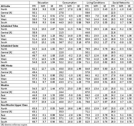
<Table 7.3>

Table 7.3 shows the values of the predicted performance index (PPI), based on SURE

estimates over data for 37,247 households, for each social group, first on an all-India basis and then

predictions”, described in chapter 2, which isolates the effect on the households’ PPI of their

belonging to different social groups. First, “pretend” that all the 37,247 households are from the SC. Holding the values of the other variables constant (either to their observed sample values, as in this

chapter, or to their mean values), predict the values of the PI for each household (for a specific

indicator) under this all-SC scenario and denote itpSC. Then pSCrepresents the predicted performance

index (PPI) for SC households. Next, “pretend” that all the 37,247 households are Muslim and, again

holding the values of the other variables constant, predict the values of the PI for each household (for

a specific indicator) under this all-Muslim scenario and denote it_pM_{. Then p}M_{represents the}

predicted performance index (PPI) for Muslim households.

Since the values of the other variables were unchanged between these two hypothetical

scenarios, the only difference between them is that, in the first scenario, the SC variable is “switched

on” (with the variables pertaining to the other groups “switched off”) — while, in the other, the

Muslim variable is “switched on” (with the variables pertaining to the other groups “switched off”) —

for all households.19 Consequently, the difference between _pSC_{and p}M_{is entirely due to differences}

between SC and Muslims. In essence, therefore, in evaluating the effect of two characteristics X and Y

on the likelihood of a particular outcome, the method of “recycled predictions” compares two

outcomes, first, under an “all have the characteristic X” scenario and, then, under an “all have the

characteristic Y” scenario. The values of the other variables remain unchanged between the scenarios.

The difference between the two probabilities could then be ascribed to the attribute represented by X

and Y (in this case, SC and Muslim).20

The columns of Table 7.3 headed ‘PPI’ show the PPI values for the five social groups, first

on an all-India basis and then for each of the five regions. The all-India values were computed using

the method of “recycled predictions”, discussed above, by assuming that all the 37,247 households in

the estimation sample belonged, successively, to each of the five social groups, with the values of the

other variables unchanged. The regional values were also computed using the method of “recycled

19

In operational terms, STATA’s margin command will perform these calculations taking into account all interaction effects.

20

predictions” but this time assuming that all the 37,247 households in the estimation sample lived in a

particular region (say, the North) and, in conjunction with this assumption, belonged, successively, to each of the five social groups, with the values of all the other variables unchanged.

With households from the NMUC as the reference group, the numbers under the column MPI

(“marginal performance index”) represent the differences between the PPI of a social group and that

of the reference group. For example, the all-India PPI for education was 48.2 for the ST and 64.7 for

the NMUC yielding an MPI for the ST of 48.2-64.7 =-16.5. The associated number under the column

headed SE (standard error) shows the standard error associated with the MPI. For the ST, this was

0.79. Dividing the MPI by its SE yields a z-value of 20.9 (not shown in the table) and this implied that

the MPI was significantly different from zero. In other words, the education PPI was significantly

lower for ST households compared to households from the NMUC.

A similar result emerges for the other social groups with respect to all the indicators. As the

other columns of Table 7.3 show, the PPI for households from the NMUC was significantly higher

than the PPI for households from the other social groups in respect of: per-capita consumers’

expenditure; living conditions; and social networks. In other words, compared to households from the

other social groups, households from the NMUC were, on average, significantly more likely to fulfil

their potential in respect of education, living standards, living conditions, and social networks. This

statement was true not just for India in its entirety but for all its regions considered separately — the

North, the Centre, the East, the West, and the South.

There was no significant difference between Muslim and SC households in their PPI for

education (respectively, 49.4 and 50.3) but the education PPI for both groups was significantly lower

than that for NMOBC households (55.9). In terms of per-capita consumption, however, the PPI for

Muslim households (31.4%) was significantly higher than that for the SC (27.5) but was significantly

lower than that for NMOBC households (34.3).

In terms of living standards, however, the PPI of Muslim households (72.9) was significantly

higher than that of SC (65.4) and of NMOBC (70.9) households and, in large part, this was explained

by the fact that Muslim households were more likely to have a toilet than households from the other

households. The results for social networks mirrored that for living conditions: the PPI of Muslim

households (24.0) was significantly higher than that of SC (20.4) and of NMOBC (21.5) households.

In large part, this was explained by the fact that Muslim households were more likely to know a

doctor or a teacher as a part of relatives/caste/community than households from the other groups: 25%

of Muslim households knew a doctor as a part of relatives/caste/community compared to 15% of SC,

and 17% of NMOBC, households and 32% of Muslim households knew a teacher as a part of

relatives/caste/community compared to 24% of SC, and 27% of NMOBC, households.

<Table 7.4>

Table 7.3 compared differences between social groups from both an all-India and a regional

perspective. Table 7.4, on the other hand, compares differences between regions from both an

all-India and a social group perspective. This table shows that, in terms of three indicators — education,

per-capita consumption, and living conditions — the PPI was significantly lower in the Central region

and highest in the North, South, and the West. Not only that: households from every social group had

a significantly lower PPI in the Central region than they did in other regions. For example, in terms of

education, Muslim and SC households had a PPI of 41.8 and 42.7, respectively, in the Central region

versus 57.7 and 54.6, respectively in the South. Similarly, in terms of education, households from the

non-Muslim upper class had a PPI of 63.2 in the Central region compared to 66.7 in the South.

7.8 Conclusions

The novelty of the results presented in this chapter is two-fold. First, by accounting for inequality both

within and between social groups, they extend the analysis of mean performance to include equity

sensitive human development indices. Second, by including living conditions and social networks, the

results go beyond the conventional catalogue of human development indicators — education, life

expectancy, and income — to encompass, arguably, a fuller view of well-being.

A persistent, and worrying, feature of the results is that they shows greater intra-group

inequality within marginalised and deprived groups — the SC, the ST, and Muslims — than among

the “privileged” NMUC. For example, the Gini coefficient for the distribution of the education PI

for the SC, and 0.458 for the ST. Similarly, the Gini coefficient for the distribution of the per-capita

consumption PI among households in the different subgroups was 0.492 for the NMUC but 0.525 for

Muslims, 0.514 for the SC, and 0.596 for the ST.

This raises issues of the existence of a “creamy layer” among the deprived groups — the

relatively wealthy members of such groups whose existence only serves to highlight the poverty of

those not in this prosperous category.21 The existence of such a “creamy layer” implies that when

allowance is made for intra-group inequality, the equally distributed index values for deprived groups

are considerably lower than their corresponding mean values. Not only are the SC/ST/Muslims

deprived, but their poverty is compounded by the fact that such prosperity as might exist among them

is captured by a privileged few among their number.

The approach that policy makers in India have taken to overcome the economic and

social “backwardness” of the SC and the ST has been two-pronged:

(a) specific measures to combat disparity, including legal safeguards against

discrimination in education and employment and the practice of untouchability;

(b) general measuresfor the economic and social development of all persons, including

persons from the SC and ST.

These policies have, undeniably, brought about improvements but, as our analysis shows,

there is considerable distance between the development levels of SC, ST, and Muslim

households on the one hand, and NMUC households on the other. Like other economically and

educationally backward sections from the higher castes, the SC, ST, and Muslims require education

and skill development to improve their economic prospects. But, unlike other deprived persons, they

face economic and social exclusion and, therefore, require additional protection in the form of

anti-discriminatory measures. However, the existence of “exclusion-induced” deprivation means that

addressing issues of economic and social exclusion is often more difficult than addressing material

poverty. Social and cultural sources of exclusion are rooted in “custom and practice”; they include the

practice of untouchability based on caste, and hostility towards Muslims based on history. In this

21

context, efforts to effect the inclusion of groups which are stigmatised faces the special difficulty of

combating actions sanctioned by religion, culture, custom, and practice.

A final word about inequality. In the past two decades India has known unprecedented rates

of economic growth with a GDP growth rate of 6.3% in 2017 “disappointing” by earlier standards.

As Deaton (2013) points out, inequality is often the consequence of progress: “not everyone gets rich

at the same time” (p.1). This can be good if inequality spurs those who have been left behind to catch

up with those ahead through say, acquiring education and skills, or migrating from the countryside to

towns and cities where the better jobs are located. In this case, inequality is a transient phenomenon

accompanying the more durable prize of economic and social progress.

However, inequality can be bad if those who have succeeded attempt to prevent others from

doing so. Then inequality becomes entrenched and leads to unrest among those who are left behind

and see little hope of catching up. There is danger, however, that this may be the case in India with

the rich and poor leading separate lives with no bridges between them. As Rao (2017) has pointed

out, “opting out of the public hospitals and government schools that they once used and benefited

from, the privileged and middle classes have made their own arrangements to meet their daily needs

by setting up private hospitals, private insurance, private schools” (p. xviii). Establishing ladders

that enable all citizens of India to climb the wall of economic and social progress is one of the most

References

Anand, S., and Sen, A.K. (1994), Human Development Index: Methodology and Measurement, Human Development Report Office Occasional Paper 12, New York: UNDP.

Anand, S., and Sen, A.K. (1997), Concepts of Human Development and Poverty: A

Multidimensional Perspective, Human Development Report 1997 Papers, New York: UNDP.

Anand, S., and Sen, A.K. (2003), “Gender Inequality in Human Development: Theories and

Measurement”, in S. Fukuda-Parr and A.K. Shiv Kumar (eds), Readings in Human Development,

Oxford: Oxford University Press.

Atkinson, A.B. (1970), “On the Measurement of Inequality”, Journal of Economic Theory, 2: 244-63.

Bros-Bobbin, C. and Borooah, V.K. (2013), “Confidence in Public Bodies, and Electoral

Participation in India”, European Journal of Development Research 25: 557-583.

Deaton, A. (2013), The Great Escape: health, wealth, and the origins of inequality, Princeton,

NJ: Princeton University Press.

Desai, S., Dubey, A., and Vanneman, R. (2015), India Human Development Survey-II,

University of Maryland and National Council of Applied Economic Research, New Delhi. Ann

Arbor, MI: Inter-university Consortium for Political and Social Research.

Frank, R.H. (1997), “The Frame of Reference as a Public Good”, Economic Journal,