Munich Personal RePEc Archive
Departure time choice equilibrium and
optimal transport problems
Akamatsu, Takashi and Wada, Kentaro and Iryo, Takamasa
and Hayashi, Shunsuke
Graduate School of Information Sciences, Tohoku University,
Institute of Industrial Science, The University of Tokyo, Department
of Civil Engineering, Kobe University
4 December 2018
Online at
https://mpra.ub.uni-muenchen.de/90361/
Departure time choice equilibrium and optimal transport
problems
✩Takashi Akamatsua,∗, Kentaro Wadab,∗, Takamasa Iryoc, Shunsuke Hayashia
aGraduate School of Information Sciences, Tohoku University, Aramaki Aoba 6-3-09, Aoba-ku, Sendai, Miyagi, Japan
980-8579.
bInstitute of Industrial Science, The University of Tokyo, Komaba 4-6-1, Meguro-ku, Tokyo, Japan 153-8505. cDepartment of Civil Engineering, Kobe University, Rokkodai-cho 1-1, Nada, Kobe, Hyogo, Japan 657-8501.
Abstract
This paper presents a systematic approach for analyzing the departure-time choice equilibrium (DTCE) problem of a single bottleneck with heterogeneous commuters. The approach is based on the fact that the DTCE is equivalently represented as a linear programming problem with a special structure, which can be analytically solved by exploiting the theory of optimal transport combined with a decomposition technique. By applying the proposed approach to several types of models with heterogeneous commuters, it is shown that the dynamic equilibrium distribution of departure times exhibits striking regularities under mild assumptions regarding schedule delay functions, in which commuters sort themselves according to their attributes, such as desired arrival times, schedule delay functions (value of times), and travel distances to a destination.
Keywords: departure time choice equilibrium, linear programming, optimal transport, sorting
1. Introduction
The modeling and analysis of rush-hour traffic congestion has a rich history, dating back
to the seminal work ofVickrey (1969). In the basic model of Vickrey, it is assumed that a
fixed number of commuters with homogeneous preferences wish to arrive at a single destination (workplace) at a same preferred time, traveling through a single route that has a bottleneck of fixed capacity. Each commuter chooses the departure time of his/her trip from home to minimize his/her generalized trip cost, including trip time, queuing delay at the bottleneck and schedule delay (i.e., costs of arriving early or late at their destination). The problem is to determine a dynamic equilibrium distribution of departure times where no commuter can reduce his/her gen-eralized cost by changing his/her departure time unilaterally. The importance of the problem in transportation planning and demand management policies has led to various extensions of the basic model to allow for (1) distributed/heterogeneous preferred departure times, (2) heterogene-ity in the valuation of travel time and schedule delay, (3) elastic demands and (4) modal/route choices.
✩Acknowledgements.
∗Corresponding author.
Email addresses:akamatsu@plan.civil.tohoku.ac.jp (Takashi Akamatsu), wadaken@iis.u-tokyo.ac.jp (Kentaro Wada)
Despite these extensive studies, however, the extant analysis approaches have some limita-tions, and are not necessarily organized into a sufficiently general theory that enables us to sys-tematically understand various extant results. Firstly, most previous studies focus only on a
sin-gle type of user heterogeneity either in the preferred arrival time (e.g.,Hendrickson and Kocur,
1981;Smith,1984;Daganzo,1985) or in the valuation of travel time and schedule delay (e.g.,
Cohen,1987;Arnott et al.,1988,1992,1994;Ramadurai et al.,2010;van den Berg and Verhoef,
2011;Liu et al.,2015;Takayama and Kuwahara,2017)1. As a result, little is known about certain
regularities of the equilibrium when there are multiple types of heterogeneity in users’ prefer-ences. Secondly, most studies restrict their analysis to a special class of schedule functions (e.g.,
a piecewise linear function)2. This is theoretically problematic since it blurs the critical
condi-tions required for the analysis results (e.g., what condicondi-tions are essential for the emergence of “sorting patterns” in the equilibrium? what conditions are required for obtaining an analytical solution?). Finally, for the models with a general schedule delay function and user heterogene-ity, systematic and efficient methods for obtaining accurate solutions are still lacking. As shown
byNie and Zhang(2009), straight-forward formulation of the model (equilibrium conditions)
results in a variational inequality problem with a non-monotone mapping, which implies that a na¨ıve numerical algorithm neither guarantees convergence nor provides accurate solutions.
This paper presents a systematic approach to analyze a wide variety of models of departure-time choice equilibrium (DTCE) with a single bottleneck. The proposed approach is based on the following two facts: (1) the equilibrium can be obtained by solving a structured linear program-ming (LP) problem and (2) the special structure of the equivalent LP allows us to apply the theory
of optimal transport (Rachev and R¨uschendorf,1998;Burkard,2007;Villani,2008), which
pro-vides explicit analytical solutions as well as efficient numerical algorithms. More specifically, we first review close relationships between DTCE and dynamic system optimal (DSO) assign-ment in a single bottleneck network, and it is shown that the DTCE with heterogeneous users can be generally constructed from the solution of the DSO assignment. Thus, the analysis of the DTCE problem is reduced to that of the DSO assignment represented as an LP. We then reveal that the equivalent LPs for various types of DTCE problems have some structural commonalities, to which the theory of optimal transport can be, either directly or indirectly, applied. Through several examples, we demonstrate how the optimal transport theory can be applied to the DTCE problems, and that the proposed approach enables us to systematically analyze basic properties of the equilibrium, such as existence, uniqueness, and some regularity of the flow patterns (e.g., temporal “sorting” patterns).
As a first example of the approach, we demonstrate that the DTCE problem with hetero-geneous preferred departure times is analytically solvable and that the sorting property of the
equilibrium flow pattern (i.e., the “First-In-First-Work principle” shown byDaganzo,1985) can
be understood from the optimal transport theory as a direct consequence of “submodularity” or the “Monge property” of the schedule cost function. As a second example, we consider the DTCE problem with heterogeneous schedule cost functions (i.e., users are differentiated accord-ing to their value of time). For this type of DTCE problem, the straightforward application of the optimal transport theory is not possible because the schedule cost functions do not satisfy the Monge property. Nevertheless, by developing an approach in which the optimal transport
1A few exceptions areNewell(1987); andLindsey(2004); but the former assumes a special class of schedule
func-tions and the latter focuses only on proving the existence and uniqueness of the equilibrium.
2Smith(1984) andDaganzo(1985) are a few exceptions; but they assume that all commuters have a same schedule
delay function.
theory is applied to the sub-problems generated from Benders decomposition of the original LP, we can show that the DTCE problem is analytically solvable under mild assumptions regarding the schedule cost function. Finally, this approach (of combining Benders decomposition with the optimal transport theory) is further extended to generalized DTCE models with two types of cost heterogeneity.
In the remainder of this article, Section2introduces a LP approach to the DTCE with
het-erogeneous commuters. Section3briefly reviews the theory of optimal transport and presents an
illustrative example of how it can be applied to analyze the DTCE problem with heterogeneous
preferred departure times. Section4analyzes the DTCE problems with heterogeneous
sched-ule delay cost functions, in which we provide a new analytical approach of combining Benders
decomposition with the optimal transport theory. Section5further extends the approach to
gen-eralized DTCE models with two types of cost heterogeneity. Concluding remarks are made in
Section6.
2. Linear programming approach to the departure time choice equilibrium problems
2.1. Departure time choice equilibrium
We consider a road network with a single O-D pair connected by one route. Users travel one
per vehicle. Users are treated as a continuum, and the total mass is denoted byQ, which is a
given constant. The route has a single bottleneck with a capacity (maximum service rate) ofµ.
The queuing congestion at the bottleneck is described by a point queue model, where a queue is assumed to form vertically at the entrance of the bottleneck. Departure time from the bottleneck
s∈ Sis assumed to be arrival time at the destination, whereS ⊂Rdenotes a sufficient arrival
time window. The free-flow travel time from the origin to the bottleneck is assumed, without
loss of generality, to be zero unless otherwise noted. Users are classified into a finite numberK
of homogeneous groups. The index set of groups is denoted byK={1,2, . . . ,K}. Let the mass
of users in groupk∈ KbeQk, then,∑
k∈KQk=Q.
Each user chooses their departure time from the bottleneck so as to minimize his/her trip cost. Trip cost is assumed to be additively separable in queuing delay cost, schedule delay cost
and free-flow travel cost. The queuing delay of users with departure timesis denoted byb(s),
and the schedule delay is defined as the difference between actual departure time and preferred departure time (work start time) from the bottleneck. The schedule delay cost function of users in
groupkmeasured in (queuing) time unit is denoted asck(s), which is assumed to be a continuous
function and is specified in the later sections. Then, the trip cost of a user in groupkdeparting
from the bottleneck at timesisb(s)+ck(s).
Under the assumptions mentioned above, thedeparture time choice equilibriumis defined
as the state in which no user could reduce his/her trip cost by changing his/her departure time unilaterally. The equilibrium condition is summarized as follows:
2.1.1. Users’ optimal choice condition
The first condition is the users’ optimal choice condition:
vk=b(s)+ck(s) if xk(s)>0
vk≤b(s)+ck(s) if xk(s)=0
∀k∈ K, ∀s∈ S (2.1)
wherevkrepresents the minimum (equilibrium) trip cost for users in groupkandxk(s)denotes
groupk’s departure flow rate from the bottleneck at times.
2.1.2. Queuing condition
In the point queue model (for the details, seeAppendix A.1), the queuing delayd(t)for a
user arriving at the bottleneck at timetcan be represented by
˙
d(t)=
λ(t)/µ−1 if d(t)>0
max.[0, λ(t)/µ−1] if d(t)=0 (2.2a)
whereλ(t)is the arrival flow rate at the bottleneck at timet. This implies that the queuing delay
should satisfy
˙
d(t)=λ(t)/µ−1 if d(t)>0
˙
d(t)≥λ(t)/µ−1 if d(t)=0 ⇔ 0≤d(t)⊥
˙
d(t)−[λ(t)/µ−1]≥0. (2.2b)
In this paper, we employ the complementarity condition (2.2b), instead of (2.2a), as the queuing delay model. This is because it is analytically tractable and its essential features are consistent
with the original point queue model (e.g., the FIFO property holds)3.
Under the assumption of a FIFO service discipline, users departing from the bottleneck at
timesarrive at the bottleneck at timeτ(s)≡s−b(s). Then, the relationship between the arrival
and departure flow rates,λ(τ(s))andx(s)≡∑
k∈Kxk(s), is as follows:
x(s)=dA(τ(s))/ds=λ(τ(s))·∆τ(s), (2.3)
whereA(t)is the cumulative arrival flow at the bottleneck at timetand∆denotes the derivative
operation with respect tobottleneck-departure-times, i.e.,
∆τ(s)≡dτ(s)/ds=1−∆b(s), ∆b(s)≡db(s)/ds
For users departing from the bottleneck at times, the queuing delayb(s)is obviously given
byb(s) = d(τ(s)), which implies∆b(s) = d(τ(s))˙ ·∆τ(s). Combining these with the queuing
delay (complementarity) condition (2.2b), we have
0≤b(s)⊥µ[∆τ(s)+ ∆b(s)]−x(s)≥0.
Sinceτ(s)+b(s)=sand thus∆τ(s)+ ∆b(s)=1, the queuing delay condition finally reduces to
the following condition:
∑
k∈Kxk(s)=µ if b(s)>0
∑
k∈Kxk(s)≤µ if b(s)=0
∀s∈ S. (2.4)
2.1.3. Flow conservation
For each user groupk, the integral of the departure flow ratexk(s)from the bottleneck must
be equal to the total massQk, that is,
∫
S
xk(s)ds=Qk ∀k∈ K. (2.5)
3SeeBan et al.(2012),Han et al.(2013) andJin(2015) for more detailed discussions.
2.2. Equivalent linear programming
The basic idea of the approach employed in this study is that the equilibrium conditions (2.1),
(2.4) and (2.5) reduce to an equivalent LP. This approach was first shown byIryo et al.(2005)
andIryo and Yoshii(2007) in a discrete time setting. We briefly describe the approach below but
for acontinuous timesetting.
Consider first the following infinite-dimensional linear programming (LP):
[2D-LP(x)] min
x≥0 .Z(x)≡
∑
k∈K ∫
S
ck(s)xk(s)ds (2.6)
subject to ∑
k∈K
xk(s)≤µ ∀s∈ S (2.7)
∫
S
xk(s)ds=Qk ∀k∈ K, (2.8)
and the associated dual problem:
[2D-LP(u,v)] max
u≥0,v.
ˇ
Z(u,v)≡ −µ
∫
S
u(s)ds+∑
k∈K
Qkvk (2.9)
subject to ck(s)+u(s)−vk≥0 ∀k∈ K, ∀s∈ S (2.10)
whereu(s)andvkare Lagrange multipliers for (2.7) and (2.8), respectively.
The problem [2D-LP(x)] represents the dynamic system optimal (DSO) assignment
prob-lem with no queuingin which total schedule delay cost is minimized subject to the capacity
constraint and flow conservation. As shown inAppendix B, the strong duality for [2D-LP(x)]
holds, implying the following complementary slackness (or optimality) conditions:
xk(s){ck(s)+u(s)−vk}=0
ck(s)+u(s)−vk≥0, xk(s)≥0 ∀k∈ K, ∀s∈ S (2.11)
u(s){µ−∑
k∈Kxk(s)}=0
µ−∑
k∈Kxk(s)≥0, u(s)≥0
∀s∈ S. (2.12)
The optimality conditions (2.11), (2.12), and (2.8) can be interpreted in several different ways. One interpretation supposes that a road manager introduces a dynamic congestion pricing scheme. Comparing the optimality conditions above and the equilibrium conditions (2.1), (2.4),
and (2.5), we easily see that replacing the queuing delaybin the equilibrium condition with the
dynamic pricesuleads to the optimality conditions. Thus, we have the following observation.
Observation 1. (Doan et al.,2011;Daganzo,2013) Suppose that the dynamic toll pattern for
passing the bottleneck is given by the optimal solutionuof [2D-LP(u,v)] (or the optimal
La-grange multiplieruof [2D-LP(x)]). Then the equilibrium under the dynamic pricing scheme
achieves the DSO flow patternx(i.e., the optimal solution of [2D-LP(x)]).
As a variant of the dynamic pricing scheme, we can also consider a time-dependent tradable permit system, which is designed to resolve the problem of congestion during the morning rush hour at a single bottleneck; it consists of the following two parts:
# of cumulative vehicle counts
D(s)
A(τ(s))
x(s)
λ(τ(s))
time s
τ(s)
u(s)
[image:7.595.207.386.138.308.2]optimal solution of [2D-LP]
Figure 1: Schematic illustration of construction of cumulative arrival curve from the solution of [2D-LP(x)]
a) the road manager issues a right that allows a permit holder to pass through the bottleneck at a pre-specified time period (“bottleneck permits”),
b) a new trading market is established for bottleneck permits differentiated by a pre-specified time
Note here that the arrival flow rate at a bottleneck at any time period is, from the definition of the scheme, equal to or less than the number of permits issued for that time period. This implies that we can completely eliminate the occurrence of queuing congestion by setting the number of permits issued per unit time to be less than or equal to the bottleneck capacity. Under the permit system, the optimality conditions (2.11), (2.12), and (2.8) can be directly interpreted as the equilibrium conditions: (2.11) represents the optimal behavior of users for a given permit
pricesu, and (2.12) represents the market clearing (demand-supply equilibrium4) condition of
the permit for departure times. This leads to the following observation.
Observation 2.(Akamatsu et al.,2006;Akamatsu,2007;Wada and Akamatsu,2010;Akamatsu and Wada, 2017) Competitive market equilibrium prices of the time-dependent tradable permits coincide
with the optimal solutionu of [2D-LP(u,v)]. Furthermore, the equilibrium under the
time-dependent tradable permit system achieves the DSO flow patternx(i.e., the optimal solution of
[2D-LP(x)]).
The two interpretations above implicitly assume for the equilibrium under the pricing scheme (or the DSO flow pattern) that there is no queuing at the bottleneck, which implies that the
departure ratesx always coincide with arrival rates at the bottleneck. However, it should be
noted that the problem [2D-LP(x)] describes no queuing mechanisms (other than the capacity constraint); hence, the arrival rates at the bottleneck need not be equal to the departure rates
x. This leads to another interpretation, in which no economic intervention of road managers is
assumed.
4For each times, the demand of time periodspermit is equal to the departure flowx(s) = ∑
k∈Kxk(s), and the
maximum supply of the permit is given by the bottleneck capacityµ.
Observation 3. (Iryo et al.,2005; Iryo and Yoshii,2007;Akamatsu et al.,2015) The optimal
solution(x,u,v)of [2D-LP(x)] and [2D-LP(u,v)] is consistent with the equilibrium conditions
if the Lagrange multiplieruin the LPs can be regarded as the queuing delaybin the equilibrium
conditions.
In order for this interpretation to be valid, arrival flow rateλat the bottleneck, which is consistent
with the queuing conditions (A.1)–(A.3) and is constructed from the optimal solution(x,u,v)
of [2D-LP(x)] (see Figure1), should be physically feasible (i.e., the arrival flow rate is
non-negative and finite). Fortunately, this is true if the schedule cost function satisfies the following
condition:∆ck(s)>−1(seeAppendix A.2andAkamatsu et al.,2015), which is consistent with
the sufficient condition for the existence of equilibria in departure-time choice models (Smith,
1984;Lindsey,2004). This condition is assumed to be satisfied throughout this paper.
3. Monge-Kantorovich problem
In order to obtaine a deeper insight into the properties (such as uniqueness, some regularity of flow patterns) of [2D-LP(x)] (or the departure time choice equilibrium), the theory of optimal
transport (see,Kantorovich,1942,1948;Rachev and R¨uschendorf,1998;Burkard,2007;Villani,
2008) is useful. In this section, we briefly review the role of Monge properties in optimization and show an illustrative example of its application to the departure time choice equilibrium.
3.1. Monge property and analytical solution
The optimal transport problem in a 2-dimensional discrete space setting is the following finite–dimensional LP, which is well known as “Hitchcock’s transportation problem” in the op-erations research and transportation fields:
[2D-OTP] min
x≥0 .Z2D(x)≡
∑
i∈I ∑
k∈K
ci,kxi,k (3.1)
subject to ∑
k∈K
xi,k=Si ∀i∈ I={1,2, . . . ,I} (3.2)
∑
i∈I
xi,k=Qk ∀k∈ K={1,2, . . . ,K} (3.3)
where vectorsSandQare given constants satisfying∑
i∈ISi=∑k∈KQk.
Before reviewing some useful theorems on the transportation problem, we introduce the fol-lowing concepts:
Definition. AnI×Kreal matrixC=[ci,k]is called aMonge matrixifCsatisfies the following property (Monge property)
ci,k+ci+
1,k+1≤ci,k+1+ci+1,k for all 1≤i<I, 1≤k<K (3.4)
Also, if the inequality in (3.4) strictly holds,Cis termed astrict Monge matrix.
Definition. A function f :R2→Rissubmodularif, and only if,
f(x,y)+ f(x′,y′)≤ f(x,y′)+f(x′,y) for allx≤x′,y≤y′ (3.5)
Also, if the inequality in (3.5) strictly holds forx <x′,y < y′, f is called astrict submodular
function.
This implies that anI×KmatrixCwhose elements are given byci,k := f(i∆x,k∆y) (1 ≤ i≤
I, 1≤k≤K)is a (strict) Monge matrix if the function f :R2→Ris (strict) submodular. Thus,
we will also term the condition (3.5) the (continuous) Monge property. If the inequalities (3.4)
and (3.5) hold in the opposite direction, then the matrixCand functionfare said to be aninverse
Monge matrix andsupermodular, respectively.
As is well known, a feasible solution to the transportation problem [2D-OTP] can always be
determined by a greedy algorithm termed thenorthwest corner rule(Hoffman,1963).
Northwest corner rule
0. Initialized the indices withi:=1andk:=1.
1. Setxi,k:=min{Si,Qk}.
2. Reduce both the supplySiand demandQkbyxi,k:Si:=Si−xi,kandQk:=Qk−xi,k.
If some ofSiandQkbecome zero, then these indices are increased by one.
3. If there still exists an unsatisfied constraint, go back to Step 2.
The Monge property further provides the following useful result:
Theorem 3.1. (Hoffman,1963,1985):If the cost matrixCof [2D-OTP] has the Monge property,
then the northwest corner rule yields an optimal solution for arbitrary supplySand demandQ
vectors.
Remarks. It is worthwhile noting thatthe cost matrix C is not used at all in the northwest
corner rule. This implies that even if we only know thatCis a Monge matrix,we can determine
an optimal solution of [2D-OTP] without knowing the explicit values of the cost coefficients. If
the cost coefficients fulfill theinverse Monge property, an optimal solution can be found by the
northeast corner rule5.
Theorem 3.2. (Dubuc et al.,1999):If the matrixC=[ci,k]in(3.1)is a strict Monge matrix, then the optimal solution of [2D-OTP] is unique (i.e., the solution provided by the northwest corner rule is the only solution of [2D-OTP]).
A continuous analogue of Theorem3.1for the continuous transportation problem is as
fol-lows. Letx∈X=Randy∈Y=Rbe random variables and letF1,F2, andFdenote the
distri-bution functions ofx,y,and(x,y), respectively. Given a continuous cost functionc:R2 →R,
the continuous optimal transport problem6can be formulated as
[2D-COTP] min
F∈F(F1,F2)
.Z2D(F)≡
∫
X×Y
c(x,y)dF(x,y) (3.6)
where F(F1,F2)≡{F(x,∞)=F1(x), F(∞,y)=F2(y),∀x,y∈R} (3.7)
Note thatF1(∞)=F2(∞).
5In the northeast corner rule, the algorithm begins with the indices withi:=1andk:=K(ori:=Iandk:=1), then
the index is decreased by one ifQk(orSi) becomes zero in Step 2 in the northwest corner rule.
6We can easily see the correspondence between the problems [2D-COTP] and [2D-OTP] by rewriting the constraints
for supply and demand in [2D-OTP] in terms ofcumulativesupply and demand (see also Subsection3.2for an example).
Theorem 3.3. (Cambanis et al.,1976;Dubuc et al.,1999)LetF1andF2be distribution functions
onR. Furthermore, suppose thatZ2D(F)is finite and the cost functionc :R2 → Ris a
sub-modular. Then an optimal solutionF∗ ∈ F(F
1,F2)is given by the so-called Fr´echet–Hoeffding
distribution
F∗(x,y)=min{F1(x),F2(y)} ∀(x,y)∈R2. (3.8)
Furthermore, if the functioncis a strict submodular, the solution is unique (i.e.,F∗(x,y)is the
only optimal solution of [2D-COTP]).
We note that the northwest corner rule for the discrete transportation problem can be viewed as explicit rules for calculating the analytical solution (i.e., Fr´echet–Hoeffding distribution) in
the discrete space setting (Burkard,2007).
3.2. Illustrative example: Model with heterogeneous preferred departure time
To illustrate the usefulness of the theory of optimal transport in analyzing the departure time choice equilibrium, we here consider the model with heterogeneous preferred departure times.
A well known sorting property of the equilibrium flow pattern, the so-calledFirst-In-First-Work
(FIFW) principle(Daganzo,1985), can be understood from the theory of optimal transport as a
direct consequence of the Monge property of the schedule cost function.
Assumption 3.1. The schedule delay cost function is assumed to be identical for all users and is given by
ck(s)≡ f(ϵ(σk,s)), ϵ(σk,s)≡s−σk, (3.9)
whereσk is the preferred departure time of users in group k and a function f : R → Ris
continuous, strictly convex, and has a minimum atϵ=0.
Lemma 3.1. Suppose that user groups are arranged (indexed) in an increasing order of their
desired arrival times:σ1<· · ·< σK. The functionck(s)defined by(3.9)satisfies the strict Monge
property.
Proof. SeeAppendix C.1.
In the above setting in which the departure time is continuous but the preferred departure time
is discrete (Newell,1987;Lindsey,2004), all groups experience queue delay to equilibrate the
trip costs of users within each group. This implies that several disjoint departure time windows can exist in equilibrium. Here we assume that a single joint departure time window (i.e., a single
rush period)S ≡ˆ [0,T] ⊂ Sof lengthT = Q/µoccurs in equilibrium7, and we focus on the
property of the departure order of users.
For the given equilibrium rush periodS ≡ˆ [0,T], the departure time choice equilibrium (i.e.,
[2D-LP(x)]) can be reduced to an instance of the optimal transport problem, whereck(s)satisfies
7This corresponds to a typical assumption that the cumulative number of users who prefer to departure by timeσ
kis
described by a continuous and differentiable S-shaped curve (e.g.,Smith,1984;Daganzo,1985).
k=1
k=2 k=3
Q1
Q2
Q3
Index k
north west time
s=0
east
northwest corner rule
F∗(κ,s)
x∗1(s)
x∗
2(s)
x∗
3(s)=µ
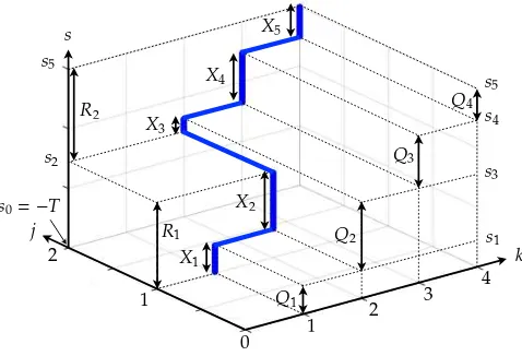
[image:11.595.183.416.143.309.2]s1 s2 s3
Figure 2: Illustration of the solution to the problem (3.13)
thestrict Monge property.
min
x≥0 .Z(x)≡
∑
k∈K ∫
s∈Sˆ
ck(s)xk(s)ds (3.10)
subject to ∑
k∈K
xk(s)=µ ∀s∈Sˆ (3.11)
∫
s∈Sˆ
xk(s)ds=Qk ∀k∈ K (3.12)
Its cumulative form is expressed as
min F∈F
∫
[1,K]×Sˆ
c(κ,s)dF(κ,s) (3.13)
where F ≡{F(κ,T)=∑
k′≤κQk′, F(K,s)=µs, ∀κ∈[1,K], ∀s∈Sˆ
}
(3.14)
Note thatF(κ,y) ≡∑
k′≤κ
∫s
0 xk′(s)ds, which is a step function ofκfor a givens. Without loss
of generality,c(κ,s)is assumed to be a continuous and strict submodular function that satisfies
c(k,s)=ck(s), ∀k=1, . . . ,K, ∀s∈S.ˆ
According to Theorem3.3, we have the following proposition:
Proposition 3.1. Suppose that Assumption3.1holds, and user groups are arranged (indexed)
in an increasing order of their desired arrival times: σ1 < · · · < σK. Then, the solution of
[2D-LP(x)] for the equilibrium rush periodSˆ is unique and its cumulative form is given by
F∗(κ,s)=min
∑
k′≤κ
Qk′, µs
∀κ∈[1,K], ∀s∈Sˆ (3.15)
# of cumulative vehicle counts
time
v3
v2
v1
Q1
Q2
Q3
0
0 =T
λ(τ(s))
u(s)
u(s)
schedule delay cost
equilibrium cost queuing delay
τ1 τ2 τ3
[image:12.595.201.394.144.392.2]s1 s2 s3
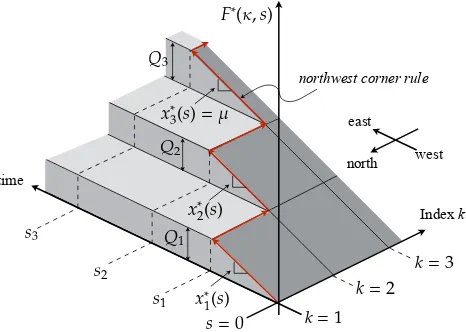
Figure 3: Optimal departure flow pattern, cost pattern, and resulting arrival flow pattern (K=3)
Using this analytical solution (3.15), we can show the regularity of the equilibrium flow pattern. Let
sk≡
∑
k′≤k
Qk′/µ (3.16)
be the time when the cumulative supplyµsis equal to the cumulative demand∑
k′≤kQk′. Then,
the following equation holds (see also Figure2):
F∗(k,sk)−F∗(k−1,sk−1)=
∫ sk
sk−1
x∗k(s)ds=µ(sk−sk−1)=Qk ∀k=1,2, . . . ,K. (3.17)
whereF(0,s0)≡0ands0 =0. This equation leads to the following proposition, i.e., the FIFW
principle.
Proposition 3.2. Suppose that the assumptions in Proposition3.1hold. Then, the equilibrium
flow patternx∗has the “sorting” property, such that all users in groupkdepart from the
bottle-neck in a time interval[sk−1,sk]of lengthQk/µand
s0≡0<s1<s2< · · · <sK−1<sK=T. (3.18)
The above “sorting” property also implies that the equilibrium cost patternv∗and the
asso-ciated queuing delaysu∗can be uniquely determined. Specifically, the following users’ optimal
choice condition within each group must hold.
v∗k=u∗(s)+ck(s) ∀s∈[sk−1,sk], ∀k∈ K. (3.19)
Then we have
v∗k:=v∗
k+1−ck+1(sk)+ck(sk) ∀k=1, . . . ,K−1. (3.20)
The recursive equation (3.20) together with a boundary condition (e.g., the queuing delay for
the last user in groupK is zero, v∗K = cK(T)), can be solved easily. Ultimately, the queuing
delayucan be determined by using Eq.(3.19). In addition, the cumulative arrival curve can be
constructed by the optimal solution(x∗,u∗,v∗)above. Figure3shows the relationships between
the optimal departure flow pattern, the cost pattern, and the resulting arrival flow pattern for the simplest case (i.e., linear schedule delay cost function).
4. Analysis of model with heterogeneous value of time
In this section, we consider the departure time choice equilibrium models in which users
have the same preferred departure timeσbut are classified intoKgroups (types) differentiated
by schedule delay cost functions. The schedule delay cost for typekusers with departure times
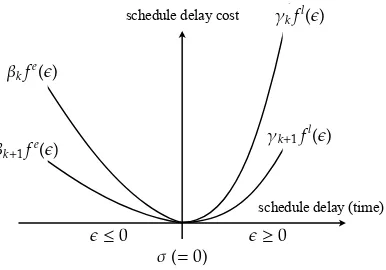
from the bottleneck is denoted byck(ϵ), whereϵ≡s−σis the schedule delay. The functionck(ϵ)
in this section is assumed to have the following form:
ck(s)=
βkfe(ϵ) if ϵ≤0 (early arrival)
γkfl(ϵ) if ϵ≥0 (late arrival) , (4.1a)
fe(0)= fl(0)=0 (4.1b)
which includes the schedule delay cost functions assumed in conventional models with
hetero-geneous users (e.g., Cohen,1987; Arnott et al.,1988,1992, 1994; van den Berg and Verhoef,
2011;Ramadurai et al.,2010;Liu et al.,2015;Takayama and Kuwahara,2017) as special cases.
For notational simplicity, the preferred departure timeσwill be set to zero in the following (i.e.,
ϵ=s).
4.1. Properties of models with no late arrivals
We first restrict ourselves to the analysis of models with the following assumption:
Assumption 4.1. fe : R → Ris a continuous decreasing function of ϵ for allϵ ≤ 0 and
fe(0)=0, fl(ϵ)→+∞for allϵ >0(i.e., late arrival is prohibited).
Lemma 4.1. Suppose that Assumption4.1holds, and that user groups are arranged (indexed) in
a decreasing order of their value of time parameters for early arrivals:β1> β2>· · ·> βK>0.
Then the functionck(s)defined by(4.1)satisfies the strict “inverse” Monge property fors≤0.
Proof. SeeAppendix C.2.
As we have seen in Section2, the departure time choice equilibrium can be obtained by
solving the linear programming problem [2D-LP(x)], whose objective is to minimize the total
schedule delay cost. Since all users have the same preferred departure timeσ, the departure
times that are closer toσare chosen at equilibrium. Thus, we obtain the following apparent
schedule delay cost
schedule delay (time)
σ(=0)
<latexit sha1_base64="SU261uWG82DfSsbpH22b1oqhEa8=">AAACqXicjZHLSsNQEIZ/473eqm4EN8GiKEqZiKAIguDGpVWrRauSxNN6MDeStKjFF/AFFFwpuBAfw40v4MJHEJcKblw4SQOi4mVCcub8Z76ZMxnDs2QQEj00KI1NzS2tbe2pjs6u7p50b99a4FZ8U+RN13L9gqEHwpKOyIcytETB84VuG5ZYN/YXovP1qvAD6Tqr4aEntmy97MiSNPWQpe1iIMu2rhbV0TmVxnbSGcpSbOp3R0ucDBJbctO3KGIXLkxUYEPAQci+BR0BP5vQQPBY20KNNZ89GZ8LHCPFbIWjBEforO7zt8y7zUR1eB/lDGLa5CoWvz6TKobpnq7pme7ohh7p7cdctThHdJdDXo06K7ydnpOBldc/KZvXEHsf1C+EhwOU+H7RHwgwwbXsf3BRryFzM3GPkmkvVqLuzTpfPTp9XpldHq6N0CU9cd8X9EC33LlTfTGvcmL5HCkenPZ1TN+dtcmsRlktN5WZn0lG2IZBDGGU5zSNeSxiCXmu6+MMF7hUxpWcUlA26qFKQ8L045Mp5jt6+5kg</latexit>
<latexit sha1_base64="SU261uWG82DfSsbpH22b1oqhEa8=">AAACqXicjZHLSsNQEIZ/473eqm4EN8GiKEqZiKAIguDGpVWrRauSxNN6MDeStKjFF/AFFFwpuBAfw40v4MJHEJcKblw4SQOi4mVCcub8Z76ZMxnDs2QQEj00KI1NzS2tbe2pjs6u7p50b99a4FZ8U+RN13L9gqEHwpKOyIcytETB84VuG5ZYN/YXovP1qvAD6Tqr4aEntmy97MiSNPWQpe1iIMu2rhbV0TmVxnbSGcpSbOp3R0ucDBJbctO3KGIXLkxUYEPAQci+BR0BP5vQQPBY20KNNZ89GZ8LHCPFbIWjBEforO7zt8y7zUR1eB/lDGLa5CoWvz6TKobpnq7pme7ohh7p7cdctThHdJdDXo06K7ydnpOBldc/KZvXEHsf1C+EhwOU+H7RHwgwwbXsf3BRryFzM3GPkmkvVqLuzTpfPTp9XpldHq6N0CU9cd8X9EC33LlTfTGvcmL5HCkenPZ1TN+dtcmsRlktN5WZn0lG2IZBDGGU5zSNeSxiCXmu6+MMF7hUxpWcUlA26qFKQ8L045Mp5jt6+5kg</latexit><latexit sha1_base64="SU261uWG82DfSsbpH22b1oqhEa8=">AAACqXicjZHLSsNQEIZ/473eqm4EN8GiKEqZiKAIguDGpVWrRauSxNN6MDeStKjFF/AFFFwpuBAfw40v4MJHEJcKblw4SQOi4mVCcub8Z76ZMxnDs2QQEj00KI1NzS2tbe2pjs6u7p50b99a4FZ8U+RN13L9gqEHwpKOyIcytETB84VuG5ZYN/YXovP1qvAD6Tqr4aEntmy97MiSNPWQpe1iIMu2rhbV0TmVxnbSGcpSbOp3R0ucDBJbctO3KGIXLkxUYEPAQci+BR0BP5vQQPBY20KNNZ89GZ8LHCPFbIWjBEforO7zt8y7zUR1eB/lDGLa5CoWvz6TKobpnq7pme7ohh7p7cdctThHdJdDXo06K7ydnpOBldc/KZvXEHsf1C+EhwOU+H7RHwgwwbXsf3BRryFzM3GPkmkvVqLuzTpfPTp9XpldHq6N0CU9cd8X9EC33LlTfTGvcmL5HCkenPZ1TN+dtcmsRlktN5WZn0lG2IZBDGGU5zSNeSxiCXmu6+MMF7hUxpWcUlA26qFKQ8L045Mp5jt6+5kg</latexit><latexit sha1_base64="SU261uWG82DfSsbpH22b1oqhEa8=">AAACqXicjZHLSsNQEIZ/473eqm4EN8GiKEqZiKAIguDGpVWrRauSxNN6MDeStKjFF/AFFFwpuBAfw40v4MJHEJcKblw4SQOi4mVCcub8Z76ZMxnDs2QQEj00KI1NzS2tbe2pjs6u7p50b99a4FZ8U+RN13L9gqEHwpKOyIcytETB84VuG5ZYN/YXovP1qvAD6Tqr4aEntmy97MiSNPWQpe1iIMu2rhbV0TmVxnbSGcpSbOp3R0ucDBJbctO3KGIXLkxUYEPAQci+BR0BP5vQQPBY20KNNZ89GZ8LHCPFbIWjBEforO7zt8y7zUR1eB/lDGLa5CoWvz6TKobpnq7pme7ohh7p7cdctThHdJdDXo06K7ydnpOBldc/KZvXEHsf1C+EhwOU+H7RHwgwwbXsf3BRryFzM3GPkmkvVqLuzTpfPTp9XpldHq6N0CU9cd8X9EC33LlTfTGvcmL5HCkenPZ1TN+dtcmsRlktN5WZn0lG2IZBDGGU5zSNeSxiCXmu6+MMF7hUxpWcUlA26qFKQ8L045Mp5jt6+5kg</latexit>
kfe(✏)
<latexit sha1_base64="0VwMZTjiNtc89Sb7NndSbBJm9JM=">AAACtXicjZHPShtRFMY/p1pjapvYbgJuQoMlhRLOiBDpKuCmS6NNIpgYZiY39pL5x8xN0A7xAfoCXXRV0UUp9iXc9AW68BGkywhuuuiZyUCxou0ZZu653z2/c+6ZY/q2DBXRxYz2YHbu4XxmIfto8fGTXH7paTP0hoElGpZne8GOaYTClq5oKKlsseMHwnBMW7TMwUZ83hqJIJSe+1Yd+qLjGPuu7EvLUCx184W2KZTRjQbj/l4kxuW28ENpe+7Lbr5EFUqseNvRU6eE1Da9/Dna6MGDhSEcCLhQ7NswEPKzCx0En7UOItYC9mRyLjBGltkhRwmOMFgd8Hefd7up6vI+zhkmtMVVbH4DJotYoR/0hSb0nb7SJf26M1eU5IjvcsirOWWF3819KGxf/5NyeFV494e6h/BxgD7fL/4DIV5xLec/uLhXxdx60qNk2k+UuHtryo/ef5xsv95aiV7QMf3kvj/TBZ1z5+7oyjqti61PyPLg9L/HdNtprlZ0quj1tVJtPR1hBst4jjLPqYoa3mATDa57hBOc4ZtW1TpaT+tPQ7WZlHmGG6Z5vwFEUp9Q</latexit>
<latexit sha1_base64="0VwMZTjiNtc89Sb7NndSbBJm9JM=">AAACtXicjZHPShtRFMY/p1pjapvYbgJuQoMlhRLOiBDpKuCmS6NNIpgYZiY39pL5x8xN0A7xAfoCXXRV0UUp9iXc9AW68BGkywhuuuiZyUCxou0ZZu653z2/c+6ZY/q2DBXRxYz2YHbu4XxmIfto8fGTXH7paTP0hoElGpZne8GOaYTClq5oKKlsseMHwnBMW7TMwUZ83hqJIJSe+1Yd+qLjGPuu7EvLUCx184W2KZTRjQbj/l4kxuW28ENpe+7Lbr5EFUqseNvRU6eE1Da9/Dna6MGDhSEcCLhQ7NswEPKzCx0En7UOItYC9mRyLjBGltkhRwmOMFgd8Hefd7up6vI+zhkmtMVVbH4DJotYoR/0hSb0nb7SJf26M1eU5IjvcsirOWWF3819KGxf/5NyeFV494e6h/BxgD7fL/4DIV5xLec/uLhXxdx60qNk2k+UuHtryo/ef5xsv95aiV7QMf3kvj/TBZ1z5+7oyjqti61PyPLg9L/HdNtprlZ0quj1tVJtPR1hBst4jjLPqYoa3mATDa57hBOc4ZtW1TpaT+tPQ7WZlHmGG6Z5vwFEUp9Q</latexit>
<latexit sha1_base64="0VwMZTjiNtc89Sb7NndSbBJm9JM=">AAACtXicjZHPShtRFMY/p1pjapvYbgJuQoMlhRLOiBDpKuCmS6NNIpgYZiY39pL5x8xN0A7xAfoCXXRV0UUp9iXc9AW68BGkywhuuuiZyUCxou0ZZu653z2/c+6ZY/q2DBXRxYz2YHbu4XxmIfto8fGTXH7paTP0hoElGpZne8GOaYTClq5oKKlsseMHwnBMW7TMwUZ83hqJIJSe+1Yd+qLjGPuu7EvLUCx184W2KZTRjQbj/l4kxuW28ENpe+7Lbr5EFUqseNvRU6eE1Da9/Dna6MGDhSEcCLhQ7NswEPKzCx0En7UOItYC9mRyLjBGltkhRwmOMFgd8Hefd7up6vI+zhkmtMVVbH4DJotYoR/0hSb0nb7SJf26M1eU5IjvcsirOWWF3819KGxf/5NyeFV494e6h/BxgD7fL/4DIV5xLec/uLhXxdx60qNk2k+UuHtryo/ef5xsv95aiV7QMf3kvj/TBZ1z5+7oyjqti61PyPLg9L/HdNtprlZ0quj1tVJtPR1hBst4jjLPqYoa3mATDa57hBOc4ZtW1TpaT+tPQ7WZlHmGG6Z5vwFEUp9Q</latexit>
<latexit sha1_base64="0VwMZTjiNtc89Sb7NndSbBJm9JM=">AAACtXicjZHPShtRFMY/p1pjapvYbgJuQoMlhRLOiBDpKuCmS6NNIpgYZiY39pL5x8xN0A7xAfoCXXRV0UUp9iXc9AW68BGkywhuuuiZyUCxou0ZZu653z2/c+6ZY/q2DBXRxYz2YHbu4XxmIfto8fGTXH7paTP0hoElGpZne8GOaYTClq5oKKlsseMHwnBMW7TMwUZ83hqJIJSe+1Yd+qLjGPuu7EvLUCx184W2KZTRjQbj/l4kxuW28ENpe+7Lbr5EFUqseNvRU6eE1Da9/Dna6MGDhSEcCLhQ7NswEPKzCx0En7UOItYC9mRyLjBGltkhRwmOMFgd8Hefd7up6vI+zhkmtMVVbH4DJotYoR/0hSb0nb7SJf26M1eU5IjvcsirOWWF3819KGxf/5NyeFV494e6h/BxgD7fL/4DIV5xLec/uLhXxdx60qNk2k+UuHtryo/ef5xsv95aiV7QMf3kvj/TBZ1z5+7oyjqti61PyPLg9L/HdNtprlZ0quj1tVJtPR1hBst4jjLPqYoa3mATDa57hBOc4ZtW1TpaT+tPQ7WZlHmGG6Z5vwFEUp9Q</latexit>
k+1fe(✏)
<latexit sha1_base64="0I7zEQ862Ojop9HXEPsEoV8xlsw=">AAACt3icjZHNTttAEMf/GNqmKS0pXCq4ICIQVVE0rpAaOEXqpUcSGkAiYNnuBlbxF/YmIliROPMCHHpqpSJVPcA7cOEFOPAIFUcqceHA2LFUAerHWPbO/nd+MzseK3BkpIguBrTBoUePn+Se5p8NP38xUng5uhL57dAWddt3/HDNMiPhSE/UlVSOWAtCYbqWI1at1vvkfLUjwkj63kfVDcSGa255siltU7FkFMYbllCmEbfe6L3mZix6sw0RRNLxvddGoUglSm3yoaNnThGZLfmFUzTwCT5stOFCwINi34GJiJ916CAErG0gZi1kT6bnAj3kmW1zlOAIk9UWf7d4t56pHu+TnFFK21zF4TdkchLTdE7f6YrO6Af9pJs/5orTHMldurxafVYExsjBq+Xrf1Iurwrbv6m/EAF20eT7JX8gwhzXcv+DS3pVzJXTHiXTQaok3dt9vrN3eLW8WJuOZ+grXXLfX+iCTrlzr/PL/lYVtc/I8+D0+2N66Ky8LelU0qvzxUo5G2EOE5jCLM/pHSr4gCXUue4+jnCME21BM7Smtt0P1QYyZgx3TNu5BWiyn8A=</latexit>
<latexit sha1_base64="0I7zEQ862Ojop9HXEPsEoV8xlsw=">AAACt3icjZHNTttAEMf/GNqmKS0pXCq4ICIQVVE0rpAaOEXqpUcSGkAiYNnuBlbxF/YmIliROPMCHHpqpSJVPcA7cOEFOPAIFUcqceHA2LFUAerHWPbO/nd+MzseK3BkpIguBrTBoUePn+Se5p8NP38xUng5uhL57dAWddt3/HDNMiPhSE/UlVSOWAtCYbqWI1at1vvkfLUjwkj63kfVDcSGa255siltU7FkFMYbllCmEbfe6L3mZix6sw0RRNLxvddGoUglSm3yoaNnThGZLfmFUzTwCT5stOFCwINi34GJiJ916CAErG0gZi1kT6bnAj3kmW1zlOAIk9UWf7d4t56pHu+TnFFK21zF4TdkchLTdE7f6YrO6Af9pJs/5orTHMldurxafVYExsjBq+Xrf1Iurwrbv6m/EAF20eT7JX8gwhzXcv+DS3pVzJXTHiXTQaok3dt9vrN3eLW8WJuOZ+grXXLfX+iCTrlzr/PL/lYVtc/I8+D0+2N66Ky8LelU0qvzxUo5G2EOE5jCLM/pHSr4gCXUue4+jnCME21BM7Smtt0P1QYyZgx3TNu5BWiyn8A=</latexit><latexit sha1_base64="0I7zEQ862Ojop9HXEPsEoV8xlsw=">AAACt3icjZHNTttAEMf/GNqmKS0pXCq4ICIQVVE0rpAaOEXqpUcSGkAiYNnuBlbxF/YmIliROPMCHHpqpSJVPcA7cOEFOPAIFUcqceHA2LFUAerHWPbO/nd+MzseK3BkpIguBrTBoUePn+Se5p8NP38xUng5uhL57dAWddt3/HDNMiPhSE/UlVSOWAtCYbqWI1at1vvkfLUjwkj63kfVDcSGa255siltU7FkFMYbllCmEbfe6L3mZix6sw0RRNLxvddGoUglSm3yoaNnThGZLfmFUzTwCT5stOFCwINi34GJiJ916CAErG0gZi1kT6bnAj3kmW1zlOAIk9UWf7d4t56pHu+TnFFK21zF4TdkchLTdE7f6YrO6Af9pJs/5orTHMldurxafVYExsjBq+Xrf1Iurwrbv6m/EAF20eT7JX8gwhzXcv+DS3pVzJXTHiXTQaok3dt9vrN3eLW8WJuOZ+grXXLfX+iCTrlzr/PL/lYVtc/I8+D0+2N66Ky8LelU0qvzxUo5G2EOE5jCLM/pHSr4gCXUue4+jnCME21BM7Smtt0P1QYyZgx3TNu5BWiyn8A=</latexit><latexit sha1_base64="0I7zEQ862Ojop9HXEPsEoV8xlsw=">AAACt3icjZHNTttAEMf/GNqmKS0pXCq4ICIQVVE0rpAaOEXqpUcSGkAiYNnuBlbxF/YmIliROPMCHHpqpSJVPcA7cOEFOPAIFUcqceHA2LFUAerHWPbO/nd+MzseK3BkpIguBrTBoUePn+Se5p8NP38xUng5uhL57dAWddt3/HDNMiPhSE/UlVSOWAtCYbqWI1at1vvkfLUjwkj63kfVDcSGa255siltU7FkFMYbllCmEbfe6L3mZix6sw0RRNLxvddGoUglSm3yoaNnThGZLfmFUzTwCT5stOFCwINi34GJiJ916CAErG0gZi1kT6bnAj3kmW1zlOAIk9UWf7d4t56pHu+TnFFK21zF4TdkchLTdE7f6YrO6Af9pJs/5orTHMldurxafVYExsjBq+Xrf1Iurwrbv6m/EAF20eT7JX8gwhzXcv+DS3pVzJXTHiXTQaok3dt9vrN3eLW8WJuOZ+grXXLfX+iCTrlzr/PL/lYVtc/I8+D0+2N66Ky8LelU0qvzxUo5G2EOE5jCLM/pHSr4gCXUue4+jnCME21BM7Smtt0P1QYyZgx3TNu5BWiyn8A=</latexit>
k+1fl(✏)
<latexit sha1_base64="FZ6fgtZB+g3zX3ZlF3mRStrCgzg=">AAACuHicjZHNSuRAEMf/xu/R1VEvghdxUJRdhsoiKHMSvHj0Y0cFR2eTbM9sM50PkszgGObg1Rfw4MmFZVm8uM/gxRfw4COIRwUvHqxkAqKyu1ZIuvrf9avqSpmekkFIdN2hdXZ19/T29WcGBj8MDWdHRjcDt+5bomi5yvW3TSMQSjqiGMpQiW3PF4ZtKrFl1pbj862G8APpOl/Cpid2baPqyIq0jJClcnaiVDVs2yhHtY96q7IXqdZsSXiBVK4zV87mKE+JTb519NTJIbVVN3uBEr7BhYU6bAg4CNlXMBDwswMdBI+1XUSs+ezJ5FyghQyzdY4SHGGwWuNvlXc7qerwPs4ZJLTFVRS/PpOTmKYr+k13dElndEOPf80VJTniuzR5Ndus8MrDR+MbD/+lbF5DfH+m/kF42EeF7xf/gQCfuJb9Di7uNWRuMelRMu0lSty91eYbB8d3G4X16WiGftAt931K13TBnTuNe+vnmlg/QYYHp78e01tn83Nep7y+Np9bWkxH2IcJTGGW57SAJaxgFUWue4hfOMcfraB91aqabIdqHSkzhhem+U+NeKA4</latexit><latexit sha1_base64="FZ6fgtZB+g3zX3ZlF3mRStrCgzg=">AAACuHicjZHNSuRAEMf/xu/R1VEvghdxUJRdhsoiKHMSvHj0Y0cFR2eTbM9sM50PkszgGObg1Rfw4MmFZVm8uM/gxRfw4COIRwUvHqxkAqKyu1ZIuvrf9avqSpmekkFIdN2hdXZ19/T29WcGBj8MDWdHRjcDt+5bomi5yvW3TSMQSjqiGMpQiW3PF4ZtKrFl1pbj862G8APpOl/Cpid2baPqyIq0jJClcnaiVDVs2yhHtY96q7IXqdZsSXiBVK4zV87mKE+JTb519NTJIbVVN3uBEr7BhYU6bAg4CNlXMBDwswMdBI+1XUSs+ezJ5FyghQyzdY4SHGGwWuNvlXc7qerwPs4ZJLTFVRS/PpOTmKYr+k13dElndEOPf80VJTniuzR5Ndus8MrDR+MbD/+lbF5DfH+m/kF42EeF7xf/gQCfuJb9Di7uNWRuMelRMu0lSty91eYbB8d3G4X16WiGftAt931K13TBnTuNe+vnmlg/QYYHp78e01tn83Nep7y+Np9bWkxH2IcJTGGW57SAJaxgFUWue4hfOMcfraB91aqabIdqHSkzhhem+U+NeKA4</latexit><latexit sha1_base64="FZ6fgtZB+g3zX3ZlF3mRStrCgzg=">AAACuHicjZHNSuRAEMf/xu/R1VEvghdxUJRdhsoiKHMSvHj0Y0cFR2eTbM9sM50PkszgGObg1Rfw4MmFZVm8uM/gxRfw4COIRwUvHqxkAqKyu1ZIuvrf9avqSpmekkFIdN2hdXZ19/T29WcGBj8MDWdHRjcDt+5bomi5yvW3TSMQSjqiGMpQiW3PF4ZtKrFl1pbj862G8APpOl/Cpid2baPqyIq0jJClcnaiVDVs2yhHtY96q7IXqdZsSXiBVK4zV87mKE+JTb519NTJIbVVN3uBEr7BhYU6bAg4CNlXMBDwswMdBI+1XUSs+ezJ5FyghQyzdY4SHGGwWuNvlXc7qerwPs4ZJLTFVRS/PpOTmKYr+k13dElndEOPf80VJTniuzR5Ndus8MrDR+MbD/+lbF5DfH+m/kF42EeF7xf/gQCfuJb9Di7uNWRuMelRMu0lSty91eYbB8d3G4X16WiGftAt931K13TBnTuNe+vnmlg/QYYHp78e01tn83Nep7y+Np9bWkxH2IcJTGGW57SAJaxgFUWue4hfOMcfraB91aqabIdqHSkzhhem+U+NeKA4</latexit><latexit sha1_base64="FZ6fgtZB+g3zX3ZlF3mRStrCgzg=">AAACuHicjZHNSuRAEMf/xu/R1VEvghdxUJRdhsoiKHMSvHj0Y0cFR2eTbM9sM50PkszgGObg1Rfw4MmFZVm8uM/gxRfw4COIRwUvHqxkAqKyu1ZIuvrf9avqSpmekkFIdN2hdXZ19/T29WcGBj8MDWdHRjcDt+5bomi5yvW3TSMQSjqiGMpQiW3PF4ZtKrFl1pbj862G8APpOl/Cpid2baPqyIq0jJClcnaiVDVs2yhHtY96q7IXqdZsSXiBVK4zV87mKE+JTb519NTJIbVVN3uBEr7BhYU6bAg4CNlXMBDwswMdBI+1XUSs+ezJ5FyghQyzdY4SHGGwWuNvlXc7qerwPs4ZJLTFVRS/PpOTmKYr+k13dElndEOPf80VJTniuzR5Ndus8MrDR+MbD/+lbF5DfH+m/kF42EeF7xf/gQCfuJb9Di7uNWRuMelRMu0lSty91eYbB8d3G4X16WiGftAt931K13TBnTuNe+vnmlg/QYYHp78e01tn83Nep7y+Np9bWkxH2IcJTGGW57SAJaxgFUWue4hfOMcfraB91aqabIdqHSkzhhem+U+NeKA4</latexit>
kfl(✏)
<latexit sha1_base64="AuU5gVWuro3lTh1ASwOTImo1GZg=">AAACtnicjZFBSxtREMf/bqu1adVoLy29SIOiIGFWCgZPgV56jEmjgtGwu77ER97uPnY3oXYJvfcL9NBTCx5EaD+El36BHvIRxGMELx6c3SyIFVtn2X3z/m9+M292bK1kGBENxoxHj8cnnkw+zT17PjU9k5+d2wz9buCIuuMrP9i2rVAo6Yl6JCMltnUgLNdWYsvuvEvOt3oiCKXvfYgOtdh1rbYnW9KxIpaa+VeNtuW6VjPu9Ft7seovNYQOpfK95Wa+QEVKbf6uY2ZOAZlV/PwpGtiHDwdduBDwELGvYCHkZwcmCJq1XcSsBezJ9FygjxyzXY4SHGGx2uFvm3c7merxPskZprTDVRS/AZPzWKA/dExD+k0ndEZX9+aK0xzJXQ55tUes0M2ZLy9rl/+lXF4jHNxQ/yA0PqLF90v+QIgVruU+gEt6jZgrpT1KpnWqJN07I7736euwtl5diBfpB51z399pQKfcude7cI42RPUbcjw48+8x3XU2V4smFc2Nt4VyKRvhJF7jDZZ4Tmso4z0qqHPdzzjCT/wySsaeIYz2KNQYy5gXuGWGvgZoRp/I</latexit><latexit sha1_base64="AuU5gVWuro3lTh1ASwOTImo1GZg=">AAACtnicjZFBSxtREMf/bqu1adVoLy29SIOiIGFWCgZPgV56jEmjgtGwu77ER97uPnY3oXYJvfcL9NBTCx5EaD+El36BHvIRxGMELx6c3SyIFVtn2X3z/m9+M292bK1kGBENxoxHj8cnnkw+zT17PjU9k5+d2wz9buCIuuMrP9i2rVAo6Yl6JCMltnUgLNdWYsvuvEvOt3oiCKXvfYgOtdh1rbYnW9KxIpaa+VeNtuW6VjPu9Ft7seovNYQOpfK95Wa+QEVKbf6uY2ZOAZlV/PwpGtiHDwdduBDwELGvYCHkZwcmCJq1XcSsBezJ9FygjxyzXY4SHGGx2uFvm3c7merxPskZprTDVRS/AZPzWKA/dExD+k0ndEZX9+aK0xzJXQ55tUes0M2ZLy9rl/+lXF4jHNxQ/yA0PqLF90v+QIgVruU+gEt6jZgrpT1KpnWqJN07I7736euwtl5diBfpB51z399pQKfcude7cI42RPUbcjw48+8x3XU2V4smFc2Nt4VyKRvhJF7jDZZ4Tmso4z0qqHPdzzjCT/wySsaeIYz2KNQYy5gXuGWGvgZoRp/I</latexit><latexit sha1_base64="AuU5gVWuro3lTh1ASwOTImo1GZg=">AAACtnicjZFBSxtREMf/bqu1adVoLy29SIOiIGFWCgZPgV56jEmjgtGwu77ER97uPnY3oXYJvfcL9NBTCx5EaD+El36BHvIRxGMELx6c3SyIFVtn2X3z/m9+M292bK1kGBENxoxHj8cnnkw+zT17PjU9k5+d2wz9buCIuuMrP9i2rVAo6Yl6JCMltnUgLNdWYsvuvEvOt3oiCKXvfYgOtdh1rbYnW9KxIpaa+VeNtuW6VjPu9Ft7seovNYQOpfK95Wa+QEVKbf6uY2ZOAZlV/PwpGtiHDwdduBDwELGvYCHkZwcmCJq1XcSsBezJ9FygjxyzXY4SHGGx2uFvm3c7merxPskZprTDVRS/AZPzWKA/dExD+k0ndEZX9+aK0xzJXQ55tUes0M2ZLy9rl/+lXF4jHNxQ/yA0PqLF90v+QIgVruU+gEt6jZgrpT1KpnWqJN07I7736euwtl5diBfpB51z399pQKfcude7cI42RPUbcjw48+8x3XU2V4smFc2Nt4VyKRvhJF7jDZZ4Tmso4z0qqHPdzzjCT/wySsaeIYz2KNQYy5gXuGWGvgZoRp/I</latexit>
<latexit sha1_base64="AuU5gVWuro3lTh1ASwOTImo1GZg=">AAACtnicjZFBSxtREMf/bqu1adVoLy29SIOiIGFWCgZPgV56jEmjgtGwu77ER97uPnY3oXYJvfcL9NBTCx5EaD+El36BHvIRxGMELx6c3SyIFVtn2X3z/m9+M292bK1kGBENxoxHj8cnnkw+zT17PjU9k5+d2wz9buCIuuMrP9i2rVAo6Yl6JCMltnUgLNdWYsvuvEvOt3oiCKXvfYgOtdh1rbYnW9KxIpaa+VeNtuW6VjPu9Ft7seovNYQOpfK95Wa+QEVKbf6uY2ZOAZlV/PwpGtiHDwdduBDwELGvYCHkZwcmCJq1XcSsBezJ9FygjxyzXY4SHGGx2uFvm3c7merxPskZprTDVRS/AZPzWKA/dExD+k0ndEZX9+aK0xzJXQ55tUes0M2ZLy9rl/+lXF4jHNxQ/yA0PqLF90v+QIgVruU+gEt6jZgrpT1KpnWqJN07I7736euwtl5diBfpB51z399pQKfcude7cI42RPUbcjw48+8x3XU2V4smFc2Nt4VyKRvhJF7jDZZ4Tmso4z0qqHPdzzjCT/wySsaeIYz2KNQYy5gXuGWGvgZoRp/I</latexit>
✏≤0
<latexit sha1_base64="d1YGnc+eS1U+b2PVZ6B1eWVWktM=">AAACrHicjZHNLgRBEMf/xvf62MVF4rKxIQ6yqREJcZK4OGItkt3NZmb00tHzYWZ2g40X8AIOToSDeAwXL+DgEcSRxMVBzewkgvioTk9X/7t+1V1TpqdkEBI9tGntHZ1d3T29qb7+gcF0Zmh4I3DrviWKlqtcf8s0AqGkI4qhDJXY8nxh2KYSm+beUnS+2RB+IF1nPTz0RMU2dhxZk5YRslTNpMvCC6RynWxZif0sVTM5ylNs2e+Onjg5JLbiZm5RxjZcWKjDhoCDkH0FAwGPEnQQPNYqaLLmsyfjc4FjpJitc5TgCIPVPf7u8K6UqA7vo5xBTFt8i+LpM5nFBN3TNT3THd3QI739mKsZ54jecsir2WKFV02fjBZe/6RsXkPsflC/EB4OUOP3RX8gwDTfZf+Di2oNmZuPa5RMe7ESVW+1+MbR6XNhYW2iOUkX9MR1n9MD3XLlTuPFuloVa2dIceP0r2367mzM5HXK66uzucX5pIU9GMM4prhPc1jEMlZQjHt5hktcaXltXStplVao1pYwI/hkWu0dhgSa2A==</latexit>
<latexit sha1_base64="d1YGnc+eS1U+b2PVZ6B1eWVWktM=">AAACrHicjZHNLgRBEMf/xvf62MVF4rKxIQ6yqREJcZK4OGItkt3NZmb00tHzYWZ2g40X8AIOToSDeAwXL+DgEcSRxMVBzewkgvioTk9X/7t+1V1TpqdkEBI9tGntHZ1d3T29qb7+gcF0Zmh4I3DrviWKlqtcf8s0AqGkI4qhDJXY8nxh2KYSm+beUnS+2RB+IF1nPTz0RMU2dhxZk5YRslTNpMvCC6RynWxZif0sVTM5ylNs2e+Onjg5JLbiZm5RxjZcWKjDhoCDkH0FAwGPEnQQPNYqaLLmsyfjc4FjpJitc5TgCIPVPf7u8K6UqA7vo5xBTFt8i+LpM5nFBN3TNT3THd3QI739mKsZ54jecsir2WKFV02fjBZe/6RsXkPsflC/EB4OUOP3RX8gwDTfZf+Di2oNmZuPa5RMe7ESVW+1+MbR6XNhYW2iOUkX9MR1n9MD3XLlTuPFuloVa2dIceP0r2367mzM5HXK66uzucX5pIU9GMM4prhPc1jEMlZQjHt5hktcaXltXStplVao1pYwI/hkWu0dhgSa2A==</latexit>
<latexit sha1_base64="d1YGnc+eS1U+b2PVZ6B1eWVWktM=">AAACrHicjZHNLgRBEMf/xvf62MVF4rKxIQ6yqREJcZK4OGItkt3NZmb00tHzYWZ2g40X8AIOToSDeAwXL+DgEcSRxMVBzewkgvioTk9X/7t+1V1TpqdkEBI9tGntHZ1d3T29qb7+gcF0Zmh4I3DrviWKlqtcf8s0AqGkI4qhDJXY8nxh2KYSm+beUnS+2RB+IF1nPTz0RMU2dhxZk5YRslTNpMvCC6RynWxZif0sVTM5ylNs2e+Onjg5JLbiZm5RxjZcWKjDhoCDkH0FAwGPEnQQPNYqaLLmsyfjc4FjpJitc5TgCIPVPf7u8K6UqA7vo5xBTFt8i+LpM5nFBN3TNT3THd3QI739mKsZ54jecsir2WKFV02fjBZe/6RsXkPsflC/EB4OUOP3RX8gwDTfZf+Di2oNmZuPa5RMe7ESVW+1+MbR6XNhYW2iOUkX9MR1n9MD3XLlTuPFuloVa2dIceP0r2367mzM5HXK66uzucX5pIU9GMM4prhPc1jEMlZQjHt5hktcaXltXStplVao1pYwI/hkWu0dhgSa2A==</latexit><latexit sha1_base64="d1YGnc+eS1U+b2PVZ6B1eWVWktM=">AAACrHicjZHNLgRBEMf/xvf62MVF4rKxIQ6yqREJcZK4OGItkt3NZmb00tHzYWZ2g40X8AIOToSDeAwXL+DgEcSRxMVBzewkgvioTk9X/7t+1V1TpqdkEBI9tGntHZ1d3T29qb7+gcF0Zmh4I3DrviWKlqtcf8s0AqGkI4qhDJXY8nxh2KYSm+beUnS+2RB+IF1nPTz0RMU2dhxZk5YRslTNpMvCC6RynWxZif0sVTM5ylNs2e+Onjg5JLbiZm5RxjZcWKjDhoCDkH0FAwGPEnQQPNYqaLLmsyfjc4FjpJitc5TgCIPVPf7u8K6UqA7vo5xBTFt8i+LpM5nFBN3TNT3THd3QI739mKsZ54jecsir2WKFV02fjBZe/6RsXkPsflC/EB4OUOP3RX8gwDTfZf+Di2oNmZuPa5RMe7ESVW+1+MbR6XNhYW2iOUkX9MR1n9MD3XLlTuPFuloVa2dIceP0r2367mzM5HXK66uzucX5pIU9GMM4prhPc1jEMlZQjHt5hktcaXltXStplVao1pYwI/hkWu0dhgSa2A==</latexit>
✏≥0
<latexit sha1_base64="iU573MCL1yN5x4A94RFUAcLQBg0=">AAACrHicjZG7SgNBFIZ/13u8JGoj2ASDYiHhrAiKlWBj6SWJQhLC7jqJg3tzdxPU4Av4AhZWihbiY6TxBSzyCGKpYGPh2c2CqHg5w+yc+ed8Z+bs0V1T+gFRu0vp7unt6x8YTAwNj4wmU2PjBd+pe4bIG47peLu65gtT2iIfyMAUu64nNEs3xY5+sBae7zSE50vHzgXHrihbWs2WVWloAUuVVLIkXF+ajp0u1cRhmiqpDGUpsvR3R42dDGLbcFItlLAHBwbqsCBgI2DfhAafRxEqCC5rZTRZ89iT0bnAKRLM1jlKcITG6gF/a7wrxqrN+zCnH9EG32Ly9JhMY4Ye6Jae6Z7u6JHefszVjHKEbznmVe+wwq0kzya3X/+kLF4D7H9QvxAujlDl94V/wMc832X9gwtrDZhbjmqUTLuRElZvdPjGyfnz9srWTHOWruiJ676kNrW4crvxYtxsiq0LJLhx6tc2fXcKC1mVsurmYmZ1OW7hAKYwjTnu0xJWsY4N5KNeXuAaN0pWySlFpdwJVbpiZgKfTKm+A3rYmtM=</latexit>
<latexit sha1_base64="iU573MCL1yN5x4A94RFUAcLQBg0=">AAACrHicjZG7SgNBFIZ/13u8JGoj2ASDYiHhrAiKlWBj6SWJQhLC7jqJg3tzdxPU4Av4AhZWihbiY6TxBSzyCGKpYGPh2c2CqHg5w+yc+ed8Z+bs0V1T+gFRu0vp7unt6x8YTAwNj4wmU2PjBd+pe4bIG47peLu65gtT2iIfyMAUu64nNEs3xY5+sBae7zSE50vHzgXHrihbWs2WVWloAUuVVLIkXF+ajp0u1cRhmiqpDGUpsvR3R42dDGLbcFItlLAHBwbqsCBgI2DfhAafRxEqCC5rZTRZ89iT0bnAKRLM1jlKcITG6gF/a7wrxqrN+zCnH9EG32Ly9JhMY4Ye6Jae6Z7u6JHefszVjHKEbznmVe+wwq0kzya3X/+kLF4D7H9QvxAujlDl94V/wMc832X9gwtrDZhbjmqUTLuRElZvdPjGyfnz9srWTHOWruiJ676kNrW4crvxYtxsiq0LJLhx6tc2fXcKC1mVsurmYmZ1OW7hAKYwjTnu0xJWsY4N5KNeXuAaN0pWySlFpdwJVbpiZgKfTKm+A3rYmtM=</latexit>
<latexit sha1_base64="iU573MCL1yN5x4A94RFUAcLQBg0=">AAACrHicjZG7SgNBFIZ/13u8JGoj2ASDYiHhrAiKlWBj6SWJQhLC7jqJg3tzdxPU4Av4AhZWihbiY6TxBSzyCGKpYGPh2c2CqHg5w+yc+ed8Z+bs0V1T+gFRu0vp7unt6x8YTAwNj4wmU2PjBd+pe4bIG47peLu65gtT2iIfyMAUu64nNEs3xY5+sBae7zSE50vHzgXHrihbWs2WVWloAUuVVLIkXF+ajp0u1cRhmiqpDGUpsvR3R42dDGLbcFItlLAHBwbqsCBgI2DfhAafRxEqCC5rZTRZ89iT0bnAKRLM1jlKcITG6gF/a7wrxqrN+zCnH9EG32Ly9JhMY4Ye6Jae6Z7u6JHefszVjHKEbznmVe+wwq0kzya3X/+kLF4D7H9QvxAujlDl94V/wMc832X9gwtrDZhbjmqUTLuRElZvdPjGyfnz9srWTHOWruiJ676kNrW4crvxYtxsiq0LJLhx6tc2fXcKC1mVsurmYmZ1OW7hAKYwjTnu0xJWsY4N5KNeXuAaN0pWySlFpdwJVbpiZgKfTKm+A3rYmtM=</latexit>
[image:14.595.204.397.139.274.2]<latexit sha1_base64="iU573MCL1yN5x4A94RFUAcLQBg0=">AAACrHicjZG7SgNBFIZ/13u8JGoj2ASDYiHhrAiKlWBj6SWJQhLC7jqJg3tzdxPU4Av4AhZWihbiY6TxBSzyCGKpYGPh2c2CqHg5w+yc+ed8Z+bs0V1T+gFRu0vp7unt6x8YTAwNj4wmU2PjBd+pe4bIG47peLu65gtT2iIfyMAUu64nNEs3xY5+sBae7zSE50vHzgXHrihbWs2WVWloAUuVVLIkXF+ajp0u1cRhmiqpDGUpsvR3R42dDGLbcFItlLAHBwbqsCBgI2DfhAafRxEqCC5rZTRZ89iT0bnAKRLM1jlKcITG6gF/a7wrxqrN+zCnH9EG32Ly9JhMY4Ye6Jae6Z7u6JHefszVjHKEbznmVe+wwq0kzya3X/+kLF4D7H9QvxAujlDl94V/wMc832X9gwtrDZhbjmqUTLuRElZvdPjGyfnz9srWTHOWruiJ676kNrW4crvxYtxsiq0LJLhx6tc2fXcKC1mVsurmYmZ1OW7hAKYwjTnu0xJWsY4N5KNeXuAaN0pWySlFpdwJVbpiZgKfTKm+A3rYmtM=</latexit>
Figure 4: Schedule delayϵ, heterogeneitiesk, and schedule delay cost
Lemma 4.2. Under Assumption4.1, the optimal solutionx∗of [2D-LP(x)] satisfies
∑
k∈Kx∗k(s)=µ if s∈S ⊂ Sˆ
∑
k∈Kx∗k(s)=0 otherwise
(4.2)
whereS ≡ˆ [−T,0]of lengthT=Q/µ.
These lemmas ensure that [2D-LP(x)] reduces to an optimal transport problem with a strict
in-verseMonge property. However, to use Theorem3.3directly, it is convenient to formulate the
op-timal transport problem as its cumulative form with a strict Monge property, as in Subsection3.2.
To do this, let us reverse the time direction:z ≡ −s; letc(κ,z)andF(κ,z)=∑
k′≤κ
∫z
0 xk′(z)dz
be the cost and distribution functions for the time windowZ=[0,T]∋z, respectively. Without
loss of generality, we also assume thatc(κ,z)is a continuous and strict submodular function that
satisfiesc(k,z)=ck(z), ∀k=1, . . . ,K, ∀z∈ Z. We then have
min
F∈F
∫
[1,K]×Z
c(κ,z)dF(κ,z) (4.3)
where F ≡{
F(κ,T)=∑
k′≤κQk′, F(K,t)=µz, ∀κ∈[1,K], ∀z∈ Z}. (4.4)
We further define the timeskwhen the cumulative supplyµzis equal to the cumulative demand
∑
k′≤kQk′, i.e.,
sk≡∑
k′≤k
Qk′/µ. (4.5)
By applying Theorem3.3to this problem, the following proposition is obtained.
Proposition 4.1. Suppose that Assumption4.1holds. Then, the flow pattern of the departure
time choice equilibrium with schedule delay cost function(4.1)has the following properties:
(1) The optimal solution of [2D-LP(x)] (i.e., equilibrium flow patternx∗) is unique and given
by the Fr´echet–Hoeffding distribution.
F∗(κ,z)=min
∑
k′≤κ
Qk′, µz
∀κ∈[1,K], ∀z∈ Z (4.6)
time
T=Q/µ
v2
c2(s)
v1
equilibrium cost
queuing delay c1(s) schedule delay cost
τw(=0) −s1
−s2
ˆ
[image:15.595.178.425.147.278.2]β1fe(−s1)
Figure 5: Graphical representation of the strong duality for [2D-LP(x)] (K=2, late arrival is prohibited)
(2) The equilibrium flow patternx∗ has the “sorting” property, such that all users in group
k depart from the bottleneck in a time interval[−sk,−sk−1] of length Qk/µ (i.e., sk =
sk−1+Qk/µ), and
−T=−sK <−sK−1< · · · <−s2<−s1<−s0≡0. (4.7)
As in the case of Subsection3.2, the equilibrium cost patternv∗and the associated queuing
delaysu∗can be uniquely determined (see Figure5).
Proposition 4.2. Suppose that Assumption4.1holds. Then, the cost pattern of the departure time
choice equilibrium with schedule delay cost function(4.1)is unique and is obtained as follows.
v∗k=∑
k′≥k
{ ˆ
βk′fe(−sk′)
}
∀k∈ K (4.8)
u∗(s)=
v∗
k−βkfe(s) ifs∈[−sk,−sk−1]
0 otherwise ∀k∈ K (4.9)
whereβkˆ ≡βk−βk+1>0andβK+1≡0.
Proof. SeeAppendix D.1.
Figure5shows the relationship between costs at equilibrium. Specifically, we can see that
the following equation holds.
∑
k∈K
(sk−sk−1)v∗k−
∫
S
u∗(s)ds=∑
k∈K
∫ −sk−1
−sk
ck(s)ds (4.10)
The first term of the LHS of Eq.(4.10) shows the total area of the rectangles below the equilibrium trip cost lines (blue bold lines) and the second term shows the red area below the queuing delay
curve (red bold line)8; the equality holds in equilibrium because the difference in the
above-mentioned two areas should be equal to the total area below the schedule delay cost curves
8The red dotted lines in Figure5are the so-calledisocost queueing curvesin the literature (Lindsey,2004).
(black bold lines). Furthermore, by recalling that(sk−sk−1)=Qk/µand multiplying both sides
of Eq.(4.10) byµ, we can see the strong duality for [2D-LP(x)].
Z(x∗)=∑
k∈K ∫
S
ck(s)x∗k(s)ds=µ
∑
k∈K
∫ −sk−1
−sk
ck(s)ds
=∑
k∈K
Qkv∗k−µ
∫
S
u∗(s)ds=Z(uˇ ∗,v∗). (4.11)
4.2. Properties of models with no early arrivals
In exactly the same manner as we have discussed above, we can consider the “reverse” case, in which the following assumption holds:
Assumption 4.2. fl : R → R is a continuous increasing function of ϵ for all ϵ ≥ 0 and
fl(0)=0, fe→+∞for allϵ <0(i.e., early arrival is prohibited).
Although this assumption (no early arrivals) may seem strange, the results for this case together with the previous (no late arrivals) case can be used as fundamental building blocks for analyzing
more general cases in Subsection4.3. As in the case of the previous subsection, the following
lemma and propositions hold.
Lemma 4.3. Suppose that Assumption4.2holds and that user groups are arranged (indexed) in
decreasing order of their value of time parameters for early arrivals:γ1 > γ2 >· · ·> γK>0.
Then, the functionck(s)defined by(4.1)satisfies the strict Monge property.
Proposition 4.3. Suppose that Assumption4.2holds. Then the flow pattern of the departure time
choice equilibrium with schedule delay cost function(4.1)has the following properties:
(1) The optimal solution of [2D-LP(x)] (i.e., equilibrium flow patternx∗) is unique and given
by the Fr´echet–Hoeffding distribution.
F∗(κ,s)=min
∑
k′≤κ
Qk′, µs
∀κ∈[1,K],∀s∈Sˆ (4.12)
whereS ≡ˆ [0,T]of lengthT=Q/µ.
(2) The equilibrium flow patternx∗ has the “sorting” property, such that all users in group
kdepart from the bottleneck in a time interval[sk−1,sk]of lengthQk/µ(i.e.,sk = sk−1+
Qk/µ), and
s0≡0<s1<s2< · · · <sK−1<sK=T (4.13)
Proposition 4.4. Suppose that Assumption4.2holds. Then, the cost pattern of the departure time
choice equilibrium with schedule delay cost function(4.1)is unique and is obtained as follows.
v∗k=∑
k′≥k
{ ˆ
γk′fl(sk′)
}
∀k∈ K (4.14)
u∗(s)=
v∗k−γkfl(s) ifs∈[sk−1,sk]
0 otherwise ∀k∈ K (4.15)
whereγkˆ ≡γk−γk+1>0andγK+1≡0.
4.3. Properties of model with early and late arrivals
We are now in a position to consider a general case in which Assumptions4.1and4.2are
relaxed to allow for both of the late and early arrivals.
Assumption 4.3. fe : R → Ris a continuous decreasing function of ϵ for allϵ ≤ 0 and
fe(0)=0, fl:R→Ris a continuous increasing function ofϵfor allϵ≥0and fl(0)=0.
Note that this assumption implies that the schedule delay cost function is strictly quasiconvex
(or unimodal), which is weaker than Assumption3.1, under which it is required to be strictly
convex.
LetH ={e,l}be the set of indices that indicate either early arrivals (e) or late arrivals (l);Xh
k
the total mass of early (ifh =e) or late (ifh =l) arrival users in groupk;Shthe time duration
s≤σifh=e,s> σifh=l. Under Assumption4.3, the problem [2D-LP(x)] can be represented
as
[2D-LP(x,X)] min
x≥0,X≥0.Z(x,X)≡
∑
k∈K ∫
S
ck(s)xk(s)ds (4.16)
subject to ∑
k∈K
xk(s)≤µ ∀s∈ S (4.17)
∫
Sh
xk(s)ds=Xhk ∀k∈ K, h∈ H (4.18)
∑
h∈H
Xhk =Qk ∀k∈ K (4.19)
Note that the equivalence between [2D-LP(x)] and [2D-LP(x,X)] is easily confirmed by
substi-tuting Eq.(4.18) into Eq.(4.19).
The properties of the problem [2D-LP(x,X)] can be analyzed using a decomposition.
Specif-ically, we first transform the problem [2D-LP(x,X)] to the following equivalent bi-level program.
min
X≥0 .
∑
h∈H
ZM(Xh) (4.20)
subject to Eq. (4.19)
where ZM(Xh)≡min
x≥0 .ZS(x|X
h)≡∑
k∈K ∫
Sh
ck(s)xk(s)ds (4.21)
subject to Eqs. (4.17) ∀s∈ Shand (4.18).
Since the lower-level (or sub-) problems (forh=eandh=l, respectively) are exactly the same
problems discussed in the previous subsections, the optimal solutionx∗ (for a givenXh) and
the associated equilibrium cost (i.e., the optimal Lagrange multiplier)(u∗,vh∗)can be obtained
analytically (see Propositions4.1–4.4). These solutions are useful in the following analysis.
Owing to the strong duality of the subproblems (i.e., Eq.(4.11)), the upper-level (or master)
problem reduces to the following problem.
min
X≥0 .
∑
h∈H
ZM(Xh)=
∑
h∈H ˇ
Z(u∗,vh∗|Xh)
=∑
h∈H
−µ
∫
Sh
u∗(s)ds+∑
k∈K
Xhkvhk∗
(4.22)
subject to Eq. (4.19)
In general, an iterative procedure is required to solve the master problem because the dual
so-lution(u∗,vh∗)is not expressed as an explicit function of the variableXh. However, thanks to
the analytical solution obtained in the previous subsections, we can explicitly transform it to a
problem including the decision variableXh.
Recall that the one-to-one correspondence between the demand distributionXhand the
equi-librium departure time vectorsh(Propositions4.1and4.3), i.e.,
sh0=0, sh
1=Xh1/µ, . . . , shk=
∑
k′≤k
Xhk′/µ, . . . , shK=Th ≡
∑
k′≤K
Xhk′/µ. (4.23)
By using these variables and the relationship (4.11), the master problem can be transformed to the following problem.
min
sh .
∑
h∈H
ZM(sh)=µ
∑
k∈K
∫ −sek−1
−se
k
ck(s)ds+µ
∑
k∈K
∫ slk
sl
k−1
ck(s)ds (4.24)
subject to 0≤sh1≤ · · · ≤shk≤ · · · ≤shK ∀h∈ H (4.25)
sek+sl
k=
∑
k≤k′
Qk′/µ ∀k∈ K (4.26)
As shown inAppendix D.2, this problem is a convex programming problem with a strict convex
objective function. We thus obtain the following lemma.
Lemma 4.4. Suppose that Assumption4.3holds. The optimal solution of the master problem is unique.
Proof. SeeAppendix D.2.
We finally obtain the following proposition.
Proposition 4.5. Suppose that Assumption4.3holds. Then the flow pattern of the departure time
choice equilibrium with schedule cost function(4.1)has the following properties:
1. The optimal solution of [2D-LP(x)] (i.e., equilibrium flow patternx∗) is unique.
2. The equilibrium flow patternx∗has the “sorting” property, such that all users in groupk
depart from the bottleneck in time intervals[sh
k−1,s
h
k],∀h∈ H, and
−Te=−se
K≤ · · · ≤ −se1≤0≤s1l ≤ · · · ≤slK=Tl. (4.27)
3. Users in all groups depart from the bottleneck both early and late (i.e., strict
inequal-ity holds in condition(4.27)), the equilibrium values ofse
kands
l
k are determined by the
following equations:
sl
k+sek=
∑
k′≤kQk′/µ
ˆ
βkfe(−sek)=γkˆ fl(sl
k)
∀k∈ K (4.28)
Proof. SeeAppendix D.3.
Note that the property 3 always holds, for example, if γk/βk = η (constant) for allk ∈ K
that is the common assumption in the literature (Vickrey,1973;Arnott et al.,1988,1992,1994;
van den Berg and Verhoef,2011;Takayama and Kuwahara,2017) (SeeAppendix D.3).
4.4. Relation to an existing semi-analytical approach
Before concluding this section, it is worthwhile mentioning a semi-analytical approach
pro-posed byLiu et al. (2015). Their approach uses the analytical solution of the model with a
piece-wise linear schedule delay function (Arnott et al.,1994) to obtain an equivalent variational
inequality (VI) problem that allows closed-form trip cost functions (or mappings). Then, the solution existence and uniqueness were examined through the VI problem. In the present frame-work, their equivalent VI corresponds to the master problem (4.22) or (4.24).
To highlight its similarities and differences with respect to the present approach concretely, let us consider the following VI, which is given as the optimality condition of the master problem (4.22):
FindX∗∈ X ≡ {X≥0and Eq.(4.19)}such that
∑
h∈H
vh∗(Xh∗)·(Xh−Xh∗)≥0 X∈ X, (4.29)
where the mappingvh∗(Xh∗)is obtained by applying the envelope theorem to the dual
subprob-lems, that is, the equilibrium trip cost function:∇ZM(Xh)=∇ZS(u∗,vh∗|Xh)=vh∗(Xh), ∀h∈
H.This is almost the same as the VI inLiu et al.(2015), except for the measurement unit of
trip cost, i.e., the problem (4.29) istime-based but that inLiu et al.(2015) ismonetary-based.
Although the monetary- and time-based formulations can be transformed in to each other by
changing the scale of schedule penalty coefficientsβkandγkfor the case ofLiu et al.(2015), the
mathematical properties of the VIs are quite different9.
More specifically, the problem (4.29) has desirable properties (see Appendix D.4 for the
proofs). The mapping of (4.29) is strictly monotone; if the schedule delay function is differen-tiable, the mapping of (4.29) is symmetric and thus a scalar potential exists for the vector field
vh∗(Xh∗), i.e.,
∑
h∈H I
0→Xh
vh∗(ω)dω
=∑
h∈H
ZM(Xh)
. (4.30)
Therefore, it is easy to obtain the uniqueness of the solutions. On the other hand, the mapping of
Liu et al.(2015)’s VI is not monotone; it is hard to establish the uniqueness property of the VI. It
9A similar conclusion has been observed in (multiclass) static traffic assignment problems (e.g.,Larsson et al.,2002).
![Figure 1: Schematic illustration of construction of cumulative arrival curve from the solution of [2D-LP(x)]](https://thumb-us.123doks.com/thumbv2/123dok_us/170500.509846/7.595.207.386.138.308/figure-schematic-illustration-construction-cumulative-arrival-curve-solution.webp)
![Figure 5: Graphical representation of the strong duality for [2D-LP(x)] (K = 2, late arrival is prohibited)](https://thumb-us.123doks.com/thumbv2/123dok_us/170500.509846/15.595.178.425.147.278/figure-graphical-representation-strong-duality-late-arrival-prohibited.webp)