Tranched Value Securities

(1)

Munich Personal RePEc Archive

Tranched Value Securities

Zvezdin, Nikolay

19 February 2019

Online at

https://mpra.ub.uni-muenchen.de/92302/

(2)

Tranched Value Securities

by

Nikolay Zvezdin1

February 19, 2019

Structured financial products and derivatives were one of the major financial innovations since 18th century, which improve market completeness by transforming risk-sharing mechanisms. Since then, thousands of derivative types were created, and its market has grown to over six-times greater than global GDP, but capital markets still exhibit efficiency only to a limited extent. This paper assesses the potential performance of Tranched Value Securities (patent pending) – a new financial instrument that transforms a single underlying to asymmetrically paying derivative, and has a potential to further improve capital markets by facilitating risk sharing, and satisfy a wide range of investment objectives.

Keywords: tranched value securities; value tranching; derivatives; securitization; risk transfer; financial instrument; structured products; securities; alternative investments; financial innovation

JEL Classification: G, G1, G10, G12, G13, G19

(3)

I. Introduction

Since the mid-18th century one of the most significant innovations in the financial world was creation of asset-backed securities (ABS), which were represented by mortgage-backed securities (MBS) in the United States where farm railroad mortgage bonds were issued2_{. Since then many other types of derivative products were created in}

an attempt to enhance risk transfer between market participants by securitizing assets or cash-flows. As a result of the advancements in structured products, global OTC derivatives market (Figure 1) has grown from nearly US$ 80 trillion in 1998 to almost US$ 700 trillion at the peak in 2011, and slightly over US$ 500 trillion in 2017, which is 6x times greater than global GDP according to IMF (January 2019).

Source: Bank for International Settlements (BIS)

Figure 1: Global OTC Derivatives Market (US$ trn).

Despite the importance and size of global derivatives market, and continuous developments, there has been little change to the actual structure of derivatives, as most of them either split various pooled assets or pooled cash-flows from the groups of assets

2_{See Riddiough, Timothy J. and Thompson, Howard E. (18/04/2012).}

250 500 750

D

er

iv

at

iv

es

O

u

ts

tan

d

in

g

-N

o

tio

n

al

A

m

o

u

n

ts

E:Equity D:Interest rate T:Credit Derivatives

L:Gold U:Other derivatives M:Other precious metals

(4)

using different types of combination of forward commitments or contingent claims with slightly modified parameters.

However, with the currently evolved technological environment it is possible to create a new type of financial instrument, that would tranch value of a single asset or a single cash-flow, resulting in creation of multiple instruments of various risk profiles all within the same asset or cash-flow, which would satisfy different types of investors – from sovereign wealth and pension funds who invest only in the safest instruments (or tranches), to speculative hedge funds aiming for high risk, high return investment opportunities. This instrument that effectively tranches a value of a single asset or cash-flow – Tranched Value Security (TVS), is expected to facilitate further improvement of risk-transfer practice, and evolution of financial system.

II. Related Literature

As shown by the various examples by Robert L. Kosowski and Salih N. Neftci (2015), current financial market accommodates different types of structured financial instruments, ranging from traditional futures and options contracts, to Quantos, volatility swaps, swaptions, and other types of hybrid instruments. Don M. Chance, PhD, CFA and Don M. Chance, PhD, CFA (2013) generalize derivative instruments to be either forward commitments, where parties fulfil an obligation in some point in future, or contingent claims which have a value in the future if a specified event occurs or given conditions are met (such as reaching a specific price by an asset). As a result of financial innovation and market development, securitization became a norm of financial practice, when multiple assets or cash-flows are pooled together, tranched and sold as different securities with various risk-return characteristics to multiple investors. Thus, different financial products have emerged, such as asset-backed securities (ABS), cash-flow backed securities, and even future flows securities3_.

Moreover, there has been a number of attempts to create innovative financial instruments or include specific contractual provisions that would change the nature of

(5)

instruments. Some examples of such are presented by Katarzyna Jakimowicz, David Osimo, and others (2017) that discuss use of co-investment schemes defined as public equity investment in private companies alongside a partner organization; blending instruments, which combine grants with either loans, soft loans, guarantees, or equity; and royalty-based financing instruments, also referred to as revenue-based financing.

Source: Dr. Helke Waelde. KWF

Figure 2: Innovative Financial Instruments.

Another overview of new financial instruments is provided by Dr. Helke Waelde (2013), where instruments can be of three types: additional public funds, which implement taxes and levies on specific activities, government auctions on rights of use,

and allocation of International Monetary Fund’s (IMF) Special Drawing Rights (SDR);

(6)

forgiveness mechanisms and debt-for-development swaps. These instruments are summarized on Figure 2, and as can be seen, they are typically modifications of existing instruments or contractual agreements, with hybrid or specialized characteristics and underlying assets. However, such instruments are mostly non-standardized, and are not easily accessible by general investment public, even though they do serve the purpose of risk-transfer when used for narrow purposes.

Besides the above instruments, there are various other equity and debt derivatives and structured products, among which Barriers, Cliquets, Autocallable, Volatility-linked, Equity-linked CDs, Baskets and Rainbow derivatives, and multiple others, all of which modify some of the more common derivative parameters and combine various products or assets under one security with diverse payment and obligation structures. This allows satisfying various risk-return appetites of different investment groups, however, none of currently available instruments is able to do so within a single asset that could serve as underlying for the same class of instrument with various risk-return profile.

This results in market incompleteness and only partial efficiency4_{, allowing for asset}

mispricing, instruments misuse and arbitrage profits for sophisticated investors. At the same time, while return pattern from a securities or derivatives can be either symmetric or asymmetric5_{, whereas symmetric implies returns that move proportionally in}

response to price changes of underlying, and asymmetric being such instrument that does not directly translate returns of underlying into a continuous linear profit-loss pattern of derivative instrument; there is a continuous increase in the demand for financial instruments with asymmetric return patterns, and the currently presented Tranched Value Security (TVS) is one of possible types of such instrument.

III. Tranched Value Securities

This section lays out some of the basic principles and parameters of the proposed new financial instrument – Tranched Value Security. First, general construction model is

4_{See Saad E.W., Prokhorov D.V., and Wunsch D.C. (November 1998).}

(7)

presented with some key attributes of TVS, with later economic valuation model and its advantages and further work required depiction.

A. TVS General Form

In perfect capital markets, TVS, similar to other derivatives would serve no purpose; as the costs of constructing and marketing it would inhibit its creation. However, market perfectness is highly questionable given the currently worsening economic conditions, and various evidences shown by Jegadeesh, N, and Titman, S. (2001), which demonstrated that some investment strategies, such as momentum in particular do produce positive risk-adjusted average returns; by multiple market anomalies, such as Calendar effects (Sell in May principle6_{, January effect}7_{, January barometer}8_{, Mark Twain}

effect9_{, Weekend effect}10_{, and several others), various asset bubbles}11_{, stock market}

crashes, and flash crushes12_{; and by existence of investors that succeed to continually}

outperform markets13_{. While some of these anomalies do fade away over time, sometimes}

they appear again on the market, while others continually persist14_{, illustrating that}

financial markets are not of strong form efficiency, and if not of weak form efficiency – they are at least semi-strong efficient15_.

All of this supports a need for further enhancement of market efficiency, which is partially possible with new financial instruments that would improve market completeness, risk transfer practice and sensitivity to new information, and Tranched Value Security is a possible candidate for this role.

6_{See Maberly, Edwin D., and Raylene M. Pierce (April 2004).}

7_{See Haugen, R. A., & Lakonishok, J. (1988).}

8_{See Christian Felde (January 2011).}

9_{See Teresa Meek (February 2017).}

10_{See Kenneth R. French (March 1980).}

11_{See Michael Simkovic (2009).}

12_{See Dragos Bozdog, Ionut Florescu, Khaldoun Khashanah, and Jim Wang (October 2018).}

13_{See John Reeves (May 2009).}

14_{See Eugene F. Fama and Kenneth R. French (2008).}

(8)

In addition to the above, recent period of low interest rates16_{, creates a need for new}

instruments that would allow to amplify risk-return profiles of various assets by artificially creating different risk-return levels within the same security, which can satisfy diverse investment groups, without necessarily packaging and repackaging a number of other securities, and increasing use of leverage, as it is currently usually done.

As such, TVS presents an opportunity for market improvement, while combining some of the properties of other currently existing structured products.

The author defines Tranched Value Security (TVS) as: a security whose income payments, and hence value is derived from and collateralized (or "backed") by the value of a single asset, group of assets, stream of cash-flows or any other entity or product possibly having a determinable value (and / or price). Value of TVS is derived either from a value share of a specific underlying, or from a minimum contract value, which can equal to the value share of a specific underlying at the contract initiation, given that a

higher-level (or “prior”) TVSs are satisfied.

Tranching the value of a single asset and creating different products allows TVS to be sold through securitization process, while diversifying underlying-specific risks by creating value tranches of various orders. This is similar to the sequential-pay collateralized mortgage obligations (CMOs), which are structured so that each tranche retires in sequence, where the payment rules for principal payment distribution are known but the exact amounts to be paid are not. TVS offers similar rules for value exercise, where first, all senior value tranches must be paid if requested (similar to exercising a call option contract), followed by the less senior tranches if anything left. Other instruments are also similar in concept to TVS that allow for credit tranching, time tranching, cash-flow tranching, asset pool tranching, with a major distinction, that with the use of TVS, the underlying does not need to be necessarily a pool of assets or a stream of various cash flows – it can be rather anything, what has a value.

The main principles of TVS are depicted on Figure 3, which is a modification of IMF’s illustration of CDO principles (2008), as TVS effectively possesses similar characteristics

(9)

to any other ABS (and CDO), but instead of using pooled assets or cash-flows as underlying, is using asset’s value, which is further subordinated.

Source: Modified according to IMF (2008).

Figure 3: TVS General Principle.

In such structure, the highest value tranches are similar to the Planned Amortization Class (PAC) tranche securities, while in the case of TVS, it is rather a Planned Value Class (PVC) tranche securities, which is designed to protect investors from sharp declines of value of their portfolios, allowing to effectively manage idiosyncratic risks. On the other hand, the lowest value tranches can be viewed as support value tranches (SVT), which exhibit the highest risks and highest expected returns. As long as the market value of underlying does not fluctuate significantly from the initial one, values of PVCs and SVTs will remain relatively stable, reducing the risk that investors’ portfolio value will deteriorate significantly, thus allowing all investors to earn relatively same return from

Senior Value Tranche

Secondary Value Tranche

Mezzanine Value Tranche Junior Value Tranche Subordinated Value Tranche

Lower

Yield First Paid Lower Risk

Higher

Yield Last Paid Higher Risk

TVS Payment Structure

(10)

the TVSs that are based on the same underlying. However, once the underlying’s value starts to exhibit significant volatility, different tranches of TVS backed by the same underlying start to display very different returns, as will be shown further.

While the main proposed structure of TVS is of perpetual nature in the case of equity instruments (with indefinite life and no expiration date), TVS issued for maturing fixed income instruments or contracts with expiration date, can also have an expiration date.

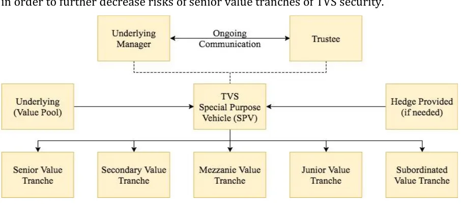
B. TVS Contractual Relations

A generic example of the contractual relationships involved in TVS are shown on Figure 4, which is modified from Schorin, C. and S. Weinreich (1998).

The trustee of the TVS is responsible for monitoring the contractual provisions of the TVS and their execution. Manager of the underlying is responsible for selection and purchase of underlying for special purpose vehicle (SPV), with subsequent tranching the value of underlying, creating multiple securities, that are held by SPV. Special purpose vehicle issues multiple securities (TVSs) that correspond to various levels of seniority of the value pool, which are sold to investors. Other roles required in TVS issuance include underwriters that acts as the structurers and arrangers, accountants that would perform a cash-flow tie-out in which the transaction's waterfall is modeled per the priority of value set forth in the transaction documents, and attorneys that ensure compliance with applicable laws and regulations and draft the transaction documents.

(11)

mechanisms can be used, such as surety bonds, wrapped securities, and letters of credit, in order to further decrease risks of senior value tranches of TVS security.

[image:11.595.71.524.135.336.2]

Source: Modified according to Schorin, C. and S. Weinreich (1998).

Figure 4: TVS Contractual Relationships.

All above, allows for efficient risk transfer and performance transformation, creating from a single instrument a series of different instruments with the same or different (depending on a particular issuance) risks from a single issue.

C. TVS Economics and Valuation

Based on the earlier presented definition and general structure of Tranched Value Securities, unconditional value of each individual TVS unit to investor is displayed by equation ( 1 )

𝑇𝑉𝑆𝑖𝑡 = max(𝑤𝑖𝑆𝑡, 𝑋𝑖) ( 1 )

Where 𝑇𝑉𝑆_𝑖_𝑡 is the value of Tranched Value Security (𝑇𝑉𝑆_𝑖), i.e. 𝑖-th value tranche at time

(12)

However, the nature of TVS conditionally tranched on the level of seniority of specific value shares implies that before the current unit of TVS can be satisfied, the previous level (more senior-level) of TVS must be satisfied, implying the model ( 2 )

𝑇𝑉𝑆𝑖𝑡 = min⁡(𝑆𝑡− 𝑇𝑉𝑆𝑖−1𝑡, max(𝑤𝑖𝑆𝑡, 𝑋𝑖)) ( 2 )

Where 𝑇𝑉𝑆_𝑖_𝑡 is the value of Tranched Value Security (𝑇𝑉𝑆_𝑖), i.e. 𝑖-th value tranche at time

𝑡 = 𝑛 of underlying (𝑆_𝑡); 𝑆_𝑡 is the price of underlying at time 𝑡 = 𝑛; 𝑤_𝑖 is the fixed weight of 𝑖-th value share corresponding to the specific underlying (𝑆_𝑡) at the contract initiation (𝑡 = 0); 𝑋_𝑖 is the minimum corresponding value of 𝑇𝑉𝑆_𝑖 share at any time, which is set fixed and equals to 𝑤_𝑖𝑆_𝑡 during the contract initiation at 𝑡 = 0; 𝑇𝑉𝑆_𝑖−1_𝑡 is the value of

higher-ranked Tranched Value Security (𝑇𝑉𝑆_𝑖), i.e. 𝑖 − 1-th value tranche at time 𝑡 = 𝑛 of underlying (𝑆_𝑡), which must be satisfied before any subsequent Tranched Value Security (𝑇𝑉𝑆_𝑖+1) can be fulfilled.

Based on this simplistic model, it is possible to illustrate price behavior of such instrument. It can be assumed that value of underlying (𝑆_𝑡=0) is US$ 100.00, for which senior value tranche security, and secondary value securities were issued. Senior value tranche security (𝑇𝑉𝑆_𝑆𝐸𝑁 ) corresponds to 60.00% value of underlying (𝑤_𝑆𝐸𝑁 = 60.00%), which is fixed and equals to 𝑤_𝑆𝐸𝑁𝑆_𝑡=0= 𝑋_𝑆𝐸𝑁 = 𝑈𝑆$⁡60.00 minimum value, or more specifically 𝑇𝑉𝑆_𝑆𝐸𝑁= max⁡(60.00% × 𝑆𝑡, 𝑈𝑆$⁡60.00); while the secondary value tranche security (𝑇𝑉𝑆_𝑆𝐸𝐶) corresponds to 1 − 𝑤_𝑆𝐸𝑁 = 𝑤_𝑆𝐸𝐶 = 40.00% value of underlying, which is fixed and equals to US$ 40.00 minimum value, or more specifically 𝑇𝑉𝑆_𝑆𝐸𝐶 =

max⁡(40.00% × 𝑆𝑡, 𝑈𝑆$⁡40.00), and can be paid only if the senior value security (𝑇𝑉𝑆𝑆𝐸𝑁) has been fully satisfied.

Based on ( 2 ), and specified initial parameters, during the contract initiation (𝑡 = 0), three securities have such values as: 𝑆_𝑡=0= 100.00, 𝑇𝑉𝑆_𝑆𝐸𝑁_𝑡=0 = 60.00, 𝑇𝑉𝑆_𝑆𝐸𝐶_𝑡=0 =

40.00. However, once market movements occur and change the price of 𝑆𝑡 to any price different from 𝑆_𝑡=0, the two 𝑇𝑉𝑆_𝑖_𝑡 change their value in a different manner. Assuming the

(13)

Figure 5: Sample Values (US$) and Returns (%) of 𝑺_𝒕=𝒏, 𝑻𝑽𝑺_𝑺𝑬𝑵_𝒕=𝒏, and 𝑻𝑽𝑺_𝑺𝑬𝑪_𝒕=𝒏.

The illustrations above clearly show that a single underlying with an observable or measurable price (and / or value, as used interchangeably in the current context) can be used to create two or more TVSs that will generate various returns even using a simplified pricing formula, which might omit some other possible aspects.

Such value model of TVS suggests the following price patterns based on the value of underlying: if 𝑆𝑡≥ 𝑋𝑖 ⟹ 𝑇𝑉𝑆𝑖_𝑡 = min⁡(𝑆𝑡− 𝑇𝑉𝑆𝑖−1_𝑡, max(𝑤𝑖𝑆𝑡, 𝑋𝑖)), and if 𝑆𝑡< 𝑋𝑖 ⟹

𝑇𝑉𝑆𝑖𝑡 = 𝑆𝑡− 𝑇𝑉𝑆𝑖−1𝑡, which also imply that if 𝑆𝑡 < 𝑇𝑉𝑆𝑖−1𝑡 ⟹ 𝑇𝑉𝑆𝑖𝑡 = 0.

However, this model omits a price premium that must be paid for receiving a superior claim right on value tranche of a particular security, which on its own is of value to investors. Under this view, the value of has three primary components: intrinsic value, time value and seniority, leading to the following conclusion ( 3 )

∑ 𝑇𝑉𝑆𝑖_𝑡 𝑡

𝑖=1

≥ 𝑆𝑡 ( 3 )

(14)

𝑇𝑉𝑆𝑖𝑡 ≥ min (𝑆𝑡− 𝑇𝑉𝑆𝑖−1𝑡, 𝑚𝑎𝑥 (𝑤𝑖

𝑆𝑡 (1 + 𝑟)𝑛,

𝑋𝑖

(1 + 𝑟)𝑛)) ( 4.1 )

Or can be extended to ( 4.2 ) in the case of perpetual TVS, which can primarily be used for equities to accommodate time value of TVS.

𝑇𝑉𝑆𝑖𝑡 ≥ min (𝑆𝑡− 𝑇𝑉𝑆𝑖−1𝑡, 𝑚𝑎𝑥 (𝑤𝑖

𝑆𝑡 𝑟 ,

𝑋𝑖

𝑟 )) ( 4.2 )

These values ( 4.1 ), ( 4.2 ) become the lower limits of the Tranched Value Security on a particular underlying, with the term 𝑆_𝑡− 𝑇𝑉𝑆_𝑖−1_𝑡 not being discounted as it already

includes the time value effect.

IV. TVS Applications

This section lays out tests conducted to verify performance of Tranched Value Securities based on the presented earlier model ( 2 ) with equity and debt instruments. First simulated results are assessed, with following case studies evaluation.

A. Simulated Results

A.1. Simulated Results: Equity Security

This section assesses performance of TVS securities issued on the basis of simulated underlying equity security (common stock). For the purpose of modeling the possible price behavior of the equity security (E), it can be assumed that the underlying has a market price of 𝐸_𝑡 at time 𝑡.𝐸_𝑡 = 𝑈𝑆$⁡100.00 at 𝑡 = 0, and has a mean periodic (expected) rate of return 𝐸(𝑟_𝑡) = 𝜇 = 0.10 with standard deviation 𝜎 = 0.50. 𝐸_𝑡 follows a lognormal distribution. Based on these inputs, 𝐸_𝑡+𝑖 was modelled using Monte Carlo simulation utilizing model ( 5 ) for 1,000 periods

𝑆𝑡 = 𝑆𝑡−1× 𝑒𝑟 ( 5 )

where 𝑟 is ( 6 )

(15)

Φ(𝑧) → 𝑝𝑟𝑜𝑏𝑎𝑏𝑖𝑙𝑖𝑡𝑦𝑜𝑓⁡𝑧 𝐹−1_{(𝑧) → 𝑧}

Furthermore, it is assumed that five Tranched Value Securities are issued from 𝐸𝑡 with characteristics presented on Figure 6.A.

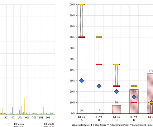
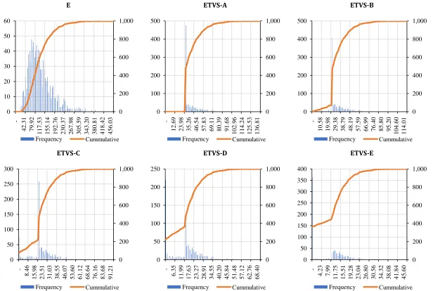
The results presented on Figure 6.A-6.G are obtained for the minimum values of five tranches of TVS and one underlying equity security. As evident, all securities experience various price fluctuations, with ETVS-A being the most stable, while ETVS-E and ETVS-D being the most volatile, at the same time experiencing defaults the most often in 37%, and 22% cases respectively out of 1,000 simulated periods. Default rates are compensated by the highest maximum returns of the three most junior value tranches (ETVS-C, ETVS-D, ETVS-E). This is the result of junior value tranches losing all value (having a market price of zero), when the value of ETVS-A becomes equal to the value of underlying equity security, due to its value seniority. ETVS Senior and ETVS Subordinated almost always have a fixed price floor (Figure 6.C) below which their value barely falls, unless the underlying equity security experiences severe price declines.

Price value distributions (Figure 6.D) and return distributions (Figure 6.F) illustrate that due to the tranching nature of the securities, and embeded protection in them against the value claim of the lower-level TVS, distribution profiles of TVSs have been transformed and do not follow the initially simulated lognormal distribution, while being highly skewed to the right, with high excess kurtosis on a return-basis, being changed to leptokurtic forms, with only the safest tranche – ETVS Senior, experiencing excess kurtosis of less than that of the underlying equity security.

(16)

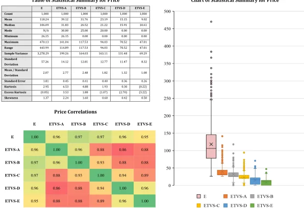
underlying equity security. Based on the statistical assessment ETVS-D generated the highest mean return, with the value of 244%, while the mean return of the underlying equity security was 24% (10.0x less than the return of ETVS-D). The lowest mean return was generated by ETVS-E due to the significant number of defaults in 37% of simulated periods, with the value of -10%. At the same time, the range of returns is the highest for ETVS-D, and ETVS-C, while for ETVS-A it is lower than even for the underlying, as this value tranche essentially contains less risk than the underlying equity security, which is evident from the twice reduced standard deviation.

(17)

Assumed Issuance Information

Security Code Value Share (%)

Minimum Value* (US$) Common Equity E 1.00 100.00

ETVS Senior ETVS-A 0.30 30.00

ETVS Subordinated ETVS-B 0.25 25.00

ETVS Junior ETVS-C 0.20 20.00

ETVS Mezzanine ETVS-D 0.15 15.00

ETVS Equity ETVS-E 0.10 10.00

Combined Price Data for Five TVSs and Underlying (US$)

TVS Price Share of Total Price of Underlying (%) Securities Performance (Limited to -100% to +500%)

Figure 6.A. Issuance, Price and Return Summary.

0 100 200 300 400 500

1 101 201 301 401 501 601 701 801 901

S

ec

u

rit

ie

s

V

al

u

es

ETVS-A ETVS-B ETVS-C ETVS-D ETVS-E E

n+

0% 20% 40% 60% 80% 100%

1 101 201 301 401 501 601 701 801 901

P

ric

e

S

h

ar

e

ETVS-A ETVS-B ETVS-C ETVS-D ETVS-E

n+ -100%

0% 100% 200% 300% 400% 500%

1 101 201 301 401 501 601 701 801 901

S

ec

u

rit

ie

s

R

et

u

rn

s

E ETVS-A ETVS-B ETVS-C ETVS-D ETVS-E

(18)

[image:18.842.218.709.86.493.2]

Securities Return Full Snapshot TVS Default Rates (When Price Equals to Zero)

Figure 6.B. Return and Default Rates (%).

-100% 9900% 19900% 29900% 39900% 49900% 59900% 69900% 79900% 89900%

1 101 201 301 401 501 601 701 801 901

S

ec

u

rit

ie

s

R

et

u

rn

s

E ETVS-A ETVS-B ETVS-C ETVS-D ETVS-E

n+

0% 1%

7%

22%

37%

0% 10% 20% 30% 40% 50% 60% 70% 80% 90% 100%

ETVS-A

ETVS-B

ETVS-C

ETVS-D

(19)

E ETVS-A ETVS-B

[image:19.842.126.512.80.483.2]

ETVS-C ETVS-D ETVS-E

Figure 6.C. Price Charts (US$) with SMA(50).

0 50 100 150 200 250 300 350 400 450 500

1

68

135 202 269 336 403 470 537 604 671 738 805 872 939

n+

0 20 40 60 80 100 120 140 160

1

68

135 202 269 336 403 470 537 604 671 738 805 872 939

n+

0 20 40 60 80 100 120

1

68

135 202 269 336 403 470 537 604 671 738 805 872 939

n+

0 20 40 60 80 100

1

68 ₁₃₅ ₂₀₂ ₂₆₉ ₃₃₆ ₄₀₃ ₄₇₀ ₅₃₇ ₆₀₄ ₆₇₁ ₇₃₈ ₈₀₅ ₈₇₂ ₉₃₉

n+

0 20 40 60 80

1

68 ₁₃₅ ₂₀₂ ₂₆₉ ₃₃₆ ₄₀₃ ₄₇₀ ₅₃₇ ₆₀₄ ₆₇₁ ₇₃₈ ₈₀₅ ₈₇₂ ₉₃₉

n+

0 10 20 30 40 50

1

68 ₁₃₅ ₂₀₂ ₂₆₉ ₃₃₆ ₄₀₃ ₄₇₀ ₅₃₇ ₆₀₄ ₆₇₁ ₇₃₈ ₈₀₅ ₈₇₂ ₉₃₉

(20)

[image:20.842.115.731.71.485.2]

Figure 6.D. Price Distribution Histograms (US$).

0 200 400 600 800 1,000 0 10 20 30 40 50 60

42.31 79.92

117.53 155.14 192.76 230.37 267.98 305.59 343.20 380.81 418.42 456.03

Frequency Сummulative

0 200 400 600 800 1,000 0 100 200 300 400 500

12.69 23.98 35.26 46.54 57.83 69.11 80.39 91.68

102.96 114.24 125.53 136.81

0 200 400 600 800 1,000 0 100 200 300 400 500

10.58 19.98 29.38 38.79 48.19 57.59 66.99 76.40 85.80 95.20 104.60 114.01

0 200 400 600 800 1,000 0 50 100 150 200 250 300 8.46

15.98 23.51 31.03 38.55 46.07 53.60 61.12 68.64 76.16 83.68 91.21

0 200 400 600 800 1,000 0 50 100 150 200 250 6.35

11.99 17.63 23.27 28.91 34.55 40.20 45.84 51.48 57.12 62.76 68.40

0 200 400 600 800 1,000 0 50 100 150 200 250 300 350 400

4.23 7.99

11.75 15.51 19.28 23.04 26.80 30.56 34.32 38.08 41.84 45.60

(21)

[image:21.842.116.712.78.487.2]

Table of Statistical Summary for Price

E ETVS-A ETVS-B ETVS-C ETVS-D ETVS-E Count 1,000 1,000 1,000 1,000 1,000 1,000

Mean 118.24 39.12 31.76 23.19 15.15 9.02

Median 106.09 31.83 26.52 21.22 15.91 10.61

Mode N/A 30.00 25.00 20.00 0.00 0.00

Minimum 26.15 26.15 0.00 0.00 0.00 0.00

Maximum 470.13 141.04 117.53 94.03 70.52 47.01

Range 443.99 114.89 117.53 94.03 70.52 47.01

Sample Variance 3,278.29 199.26 164.03 163.11 131.48 69.29

Standard

Deviation 57.26 14.12 12.81 12.77 11.47 8.32 Mean / Standard

Deviation 2.07 2.77 2.48 1.82 1.32 1.08 Standard Error 1.81 0.45 0.41 0.40 0.36 0.26

Kurtosis 2.95 6.53 4.88 1.93 0.30 (0.22)

Excess Kurtosis (0.05) 3.53 1.88 (1.07) (2.70) (3.22)

Skewness 1.37 2.24 1.60 0.60 0.42 0.50

Chart of Statistical Summary for Price

Price Correlations

E ETVS-A ETVS-B ETVS-C ETVS-D ETVS-E

E 1.00 0.96 0.97 0.97 0.96 0.95

ETVS-A 0.96 1.00 0.96 0.88 0.86 0.88

ETVS-B 0.97 0.96 1.00 0.93 0.88 0.88

ETVS-C 0.97 0.88 0.93 1.00 0.94 0.89

ETVS-D 0.96 0.86 0.88 0.94 1.00 0.96

ETVS-E 0.95 0.88 0.88 0.89 0.96 1.00

(22)

[image:22.842.112.728.68.486.2]

Figure 6.F. Return Distribution Histograms (%).

0 200 400 600 800 1,000 0 10 20 30 40 50 60 70

(0.92) (0.18) 0.49 1.15 1.81 2.47 3.13 3.80 4.46 5.12 5.78 6.44 7.11

0 200 400 600 800 1,000 0 50 100 150 200 250

(0.79) (0.47) (0.20) 0.08 0.36 0.64 0.92 1.20 1.48 1.76 2.03 2.31 2.59

0 200 400 600 800 1,000 0 50 100 150 200 250

(1.00) 0.13 1.13 2.13 3.14 4.14 5.14 6.14 7.15 8.15 9.15 10.15 11.16

0 200 400 600 800 1,000 0 100 200 300 400 500 600 700 800 900

(1.00) 28.56 54.83 81.11

107.38 133.65 159.93 186.20 212.47 238.75 265.02 291.30 317.57

0 200 400 600 800 0 100 200 300 400 500 600 700

(1.00) 78.57

149.30 220.03 290.76 361.49 432.22 502.95 573.68 644.41 715.14 785.88 856.61

0 100 200 300 400 500 600 700 0 50 100 150 200 250

(1.00) 1.32 3.38 5.43 7.49 9.55 11.61 13.67 15.73 17.79 19.85 21.91 23.97

(23)

[image:23.842.120.724.71.481.2]

Table of Statistical Summary for Return

E ETVS-A ETVS-B ETVS-C ETVS-D ETVS-E Count 999 999 999 999 999 999

Mean 0.24 0.09 0.19 0.99 2.44 (0.10)

Median 0.01 0.00 0.00 0.00 (0.16) (0.35)

Mode N/A 0.00 0.00 (1.00) (1.00) (1.00)

Minimum (0.92) (0.79) (1.00) (1.00) (1.00) (1.00)

Maximum 7.36 2.70 11.53 327.42 883.13 24.74

Range 8.28 3.48 12.53 328.42 884.13 25.74

Sample Variance 0.78 0.22 1.05 152.01 1,715.85 3.10

Standard

Deviation 0.27 0.19 0.19 0.08 0.06 (0.06) Standard Error 0.03 0.01 0.03 0.39 1.31 0.06

Kurtosis 8.56 4.60 53.47 548.59 393.36 91.84

Excess Kurtosis 5.56 1.60 50.47 545.59 390.36 88.84

Skewness 2.23 1.66 6.18 21.93 19.72 8.16

Chart of Statistical Summary for Return

* Outliers for E, ETVS-B, ETVS-C, ETVS-D, ETVS-E amounting to > 3.0x are excluded for display purposes

Return Correlations

E ETVS-A ETVS-B ETVS-C ETVS-D E

E 1.00 0.82 0.78 0.23 0.08 0.53

ETVS-A 0.82 1.00 0.57 0.13 0.04 0.46

ETVS-B 0.78 0.57 1.00 0.13 0.04 0.47

ETVS-C 0.23 0.13 0.13 1.00 0.05 0.48

ETVS-D 0.08 0.04 0.04 0.05 1.00 0.51

[image:23.842.402.726.78.451.2]

ETVS-E 0.53 0.46 0.47 0.48 0.51 1.00

(24)

A.2. Simulated Results: Fixed Income Security

This section assesses the performance of TVS securities issued on the basis of simulated underlying fixed-income (debt) security. For the purpose of modeling the possible price behavior of the debt security (D), it can be assumed that it has the following characteristics: Face Value (FV) = US$ 100.00, Maturity (N) = 1,000 days = 2.74 years, Coupons (C) = 0.05 annually, Yield-to-Maturity (YTM) = 0.05 at 𝑡 = 0, the resulting Present Value (PV) = US$ 100.00 at 𝑡 = 0. Furthermore, it is assumed that YTM has a standard deviation 𝜎 = 0.10, and 𝐸(𝑌𝑇𝑀) = 𝜇 = 0.05. For the purpose of simplicity, it is assumed that 𝑌𝑇𝑀 follows a lognormal distribution. Based on these inputs, YTM was modelled using Monte Carlo simulation utilizing model ( 5 ) for 1,000 periods.

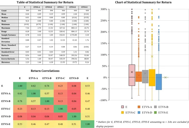
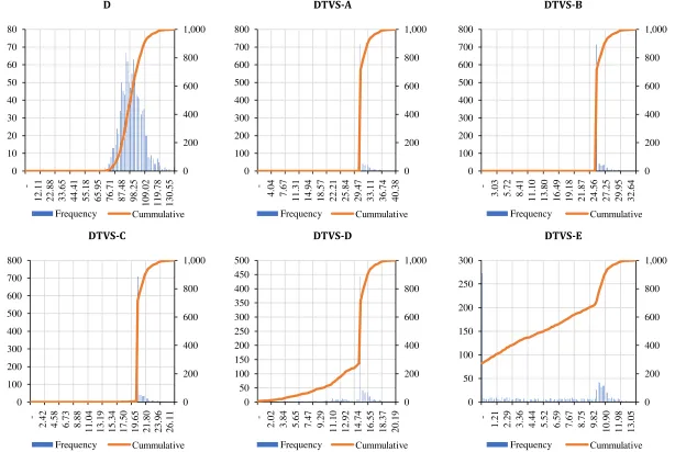
Furthermore, it is assumed that five Tranched Value Securities are issued from 𝐷𝑡 with characteristics presented on Figure 7.A. The results presented on Figure 7.A-7.G are obtained for the minimum values of five tranches of TVS and one underlying debt security.

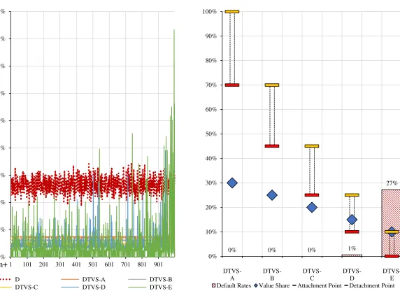
As evident, securities experience various price fluctuations (Figure 7.A), but DTVS-A, DTVS-B, and DTVS-C have a clear price floor (Figure 7.B) below which they never decline (only DTVS-C declined insignificantly several times) as the yields increase, while the underlying, and two junior value tranches continually experience value fluctuations bellow the initial PV at issuance. As a result, DTVS-D and DTVS-E experienced market price of zero multiple times amounting to 1% and 27% respectively (Figure 7.B). The default rates are compensated by the highest maximum yields with the values of 8% and 17% for DTVS-D and DTVS-E respectively (Figure 7.B, Figure 7.G).

(25)

Correlations between the securities prices (Figure 7.E) reveals that three the most senior value tranches of debt underlying have perfect positive correlation of 0.99-1.00 with each other, while two the most junior value tranches have positive but less strong correlation with all other securities. YTM correlations (Figure 7.G) depict exactly the same picture for DTVS-A, DTVS-B, DTVS-C pairs, and DTVS-D, DTVS-E pairs, while all TVSs have imperfect positive correlation with the underlying debt security.

Based on the statistical assessment ETVS-E generated the highest maximum YTM, with the value of 17%, while the maximum return of the underlying debt⁡security was 7% (2.4x less than the YTM of ETVS-E). At the same time, all securities generated nearly the same mean YTM of 1%, except for the underlying with the value of 5%.

(26)

Security Code Value Share (%)

Minimum Value* (US$) Fixed Income D 1.00 100.00

DTVS Senior DTVS-A 0.30 30.00

DTVS Subordinated DTVS-B 0.25 25.00

DTVS Junior DTVS-C 0.20 20.00

DTVS Mezzanine DTVS-D 0.15 15.00

DTVS Equity DTVS-E 0.10 10.00

TVS Price Share of Total Price of Underlying (%) Securities YTM (Limited to 0% to +8%)

0 20 40 60 80 100 120 140

1 101 201 301 401 501 601 701 801 901

S

ec

u

rit

ie

s

V

al

u

es

DTVS-A DTVS-B DTVS-C DTVS-D DTVS-E D

n+

0% 20% 40% 60% 80% 100%

1 101 201 301 401 501 601 701 801 901

P

ric

e

S

h

ar

e

DTVS-A DTVS-B DTVS-C DTVS-D DTVS-E

n+

0% 1% 2% 3% 4% 5% 6% 7% 8%

1 101 201 301 401 501 601 701 801 901

S

ec

u

rit

is

es

R

et

u

rn

s

D DTVS-A DTVS-B DTVS-C DTVS-D DTVS-E

(27)

[image:27.842.145.717.84.500.2]

Securities YTM Full Snapshot TVS Default Rates (When Price Equals to Zero)

0% 2% 4% 6% 8% 10% 12% 14% 16% 18%

1 101 201 301 401 501 601 701 801 901

S

ec

u

ri

ti

es

Re

tu

rn

s

D DTVS-A DTVS-B DTVS-C DTVS-D DTVS-E

n+

0% 0% 0% 1%

27%

0% 10% 20% 30% 40% 50% 60% 70% 80% 90% 100%

DTVS-A

DTVS-B

DTVS-C

DTVS-D

(28)

27 D D T V S -A D T V S -B D T V S -C D T V S -D D T V S -E F igu re 7 .C . P ri ce C h a rt s ( U S $) w it h S M A (5 0 ).

0 20 40 60 80

100 120 140