What do phone embeddings learn about Phonology?

Proceedings of the 16th Workshop on Computational Research in Phonetics, Phonology, and Morphology, pages 160–169

160

What do phone embeddings learn about Phonology?

Sudheer Kolachina

[email protected]

Lilla Magyar

[email protected]

Abstract

Recent work has looked at evaluation of phone embeddings using sound analogies and corre-lations between distinctive feature space and embedding space. It has not been clear what aspects of natural language phonology are learnt by neural network inspired distributed representational models such asword2vec. To study the kinds of phonological relation-ships learnt by phone embeddings, we present artificial phonology experiments that show that phone embeddings learn paradigmatic re-lationships such as phonemic and allophonic distribution quite well. They are also able to capture co-occurrence restrictions among vowels such as those observed in languages with vowel harmony. However, they are un-able to learn co-occurrence restrictions among the class of consonants.

1 Introduction

Over the last few years, distributed represen-tation models based on neural networks such

as word2vec (Mikolov et al., 2013a) and

GloVe (Pennington et al., 2014) have been of much importance in speech and natural language processing (NLP). The word2vec technique is a shallow neural network that takes a text corpus as input and outputs a vector space containing all unique words in the text. The dense vector rep-resentations of words induced using word2vec

have been shown to capture multiple degrees of similarities between words. Mikolov et al. (2013a,b) show that word embeddings can solve word analogy questions and sentence completion tasks. Mikolov et al. (2013b) show that word embeddings represent words in continuous space, making it possible to perform algebraic opera-tions, such as vector(King)−vector(Man)+ vec-tor(Woman)=vector(Queen). Considerable atten-tion has been paid to evaluating these vector

rep-resentations using human judgement datasets ( Ba-roni et al.,2014;Levy et al.,2015).Asr and Jones (2017) use artificial language experiments to study the difference between similarity and relatedness in evaluating distributed semantic models. Phone

embeddings induced from phonetic corpora have

been used in tasks such as word inflection ( Sil-fverberg et al., 2018) and sound sequence align-ment (Sofroniev and C¸ ¨oltekin,2018). Silfverberg et al. (2018) show that dense vector representa-tions of phones learnt using various techniques are able to solve analogies such aspis tobastis to X, whereX=d. They also show that there is a significant correlation between distinctive feature space and the phone embedding space.

Our goal in this paper is to understand better the evaluation of phone embeddings. We argue that significant correlation between distinctive feature space and phone embedding space cannot be auto-matically interpreted as the model’s ability to cap-ture facts about the phonology of natural language. Since many distinctive features tend to be pho-netically based, natural classes denoted by these features capture phonetic factsas well as

phono-logical facts. For example, the feature [±long]

phonol-ogy, the role of distinctive features and the task of distinctive feature/phoneme induction accrue from our experiments.

2 Background and Related work

One major difference between words and phones is that while words are meaningful units in lan-guage, phones have no meaning in themselves. However, as with words, there are clear patterns of organization of individual phones in a language. One well-known pattern in phonology is the dis-tinction betweencontrastiveandcomplementary distribution. Two phones are said to be in trastive distribution if they occur in the same con-text and create a meaning contrast. For example, b andkoccur in word-initial position and create a contrast in meaning, such as inbætversuskæt. This is why they are considered distinct phonemes in the language. On the other hand,phandpnever occur in the same context, which is referred to as being in complementary distribution. Since they are phonetically related, they are considered

allo-phones, variants of the same underlying phoneme.

The notions of contrastive and complementary dis-tribution are purely based on context. They can be considered instances of paradigmatic similar-ity discussed in the distributed semantic literature. Allophony also involves the notion of phonetic similarity. Another pattern in natural language phonology is that ofco-occurrence restrictions. A well-known example is homorganic consonant clusters. For example, in nasal plus stop clusters, the nasal must have identical place of articulation to the following stop. Yet another example of co-occurrence restriction in phonology is the phe-nomenon of vowel harmony. In some languages, a word can only have vowels which agree with re-spect to certain features, such as backness, round-ing or height. Co-occurrence restrictions can be considered to be instances of syntagmatic similar-ity whereby words that frequently occur together form a syntagm (phrase). Again, most types of co-occurrence restrictions involve phonetic similarity. The traditional method to describe phones in phonology is in terms of distinctive fea-tures (Jakobson et al.,1951). Distinctive features allow phones to be grouped intonatural classes, which are established on the basis of participa-tion in common phonological processes. They allow for generalizations about phonotactic con-texts to be captured in an economical way. In

ad-dition to distinctive features in phonology, there are also phonetic features that describe the artic-ulatory and acoustic properties of phones ( Lade-foged and Johnson,2010). However, in practice, there is considerable overlap between phonologi-cal distinctive features and phonetic features. This already poses an interesting question about the nature of the relationship between phonetics and phonology, which as we will see, is relevant to the evaluation of phone embeddings.

Next, let us examine the notion of correlation between distinctive feature space and phone em-bedding space to evaluate phone emem-beddings as proposed by Silfverberg et al. (2018). Pair-wise featural similarity is estimated using a metric such as Hamming distance or Jaccard index applied to feature representations of phones. Pair-wise con-textual similarity is estimated as cosine similar-ity between phone embeddings induced using a technique like word2vec. The correlation be-tween pairwise featural similarity and pairwise contextual similarity is estimated using Pearson’s r or Spearman’s ρ. The value of this correla-tion is shown for a number of languages in ta-ble 1. Data for Shona and Wargamay are taken fromHayes and Wilson(2008)1. Similar datasets were constructed for Telugu and the Vedic va-riety of Sanskrit2. For English, the CMU pho-netic dictionary was used with a feature represen-tation based on Parrish (2017) with some minor extensions. The word2vec implementation in the Gensim toolkit (Reh˚uˇrek and Sojkaˇ ,2010) was used to induce phone embeddings using the fol-lowing parameters- CBOW, dimensionality of30, window size of 4, negative sampling of 3, mini-mum count of 5, learning rate of 0.05. We use CBOW which predicts the most likely phone given a context of4phones in either direction as this is intuitively similar to the task of a phonologist. It would be interesting to compare CBOW and Skip-gram architectures and also, study the effect of dif-ferent parameters on this correlation between dis-tinctive feature space and phone embedding space. However, this is not the goal of our study. In this paper, we restrict our attention to the linguistic sig-nificance of this correlation.

All languages in Table1show a significant pos-itive correlation between distinctive feature space

1

https://linguistics.ucla.edu/people/ hayes/Phonotactics/index.htm#simulations

2_{Datasets and code available at https://github.}

Language Size Pearson Spearman

English 135091 0.589 0.612

Shona 4395 0.431 0.575

Telugu 19627 0.349 0.350

Wargamay 5910 0.411 0.428

Vedic 45334 0.351 0.285

English 4000 0.129 0.161

Shona 4000 0.507 0.533

Telugu 4000 0.202 0.206

Wargamay 4000 0.219 0.387

Vedic 4000 0.146 0.159

Table 1: Correlation between distinctive feature space and embedding space, all values significant (p <0.01)

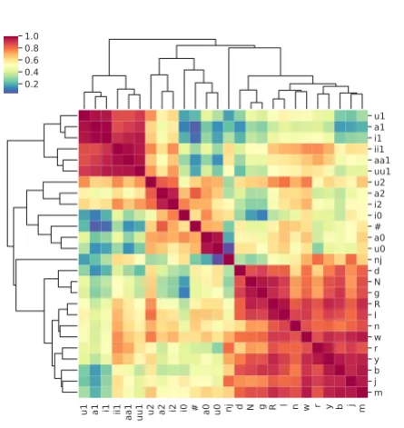
and embedding space. What is the physical inter-pretation of this correlation? Firstly, it is impor-tant to note the use of this correlation to evaluate phone embeddings presupposes that these hand-crafted distinctive features are the gold standard descriptions of the phonology of these languages. Even if this were the case, the kind of distinc-tive features used to describe phones plays an im-portant role in the interpretation of this correla-tion. If feature specifications of phones are based mostly on their phonetic properties, a positive cor-relation between featural space and embedding space indicates that phonetically similar phones tend to occur in similar contexts. In other words, the natural classes of phonology are tightly con-strained by phonetics. To illustrate this point, we take the example of Wargamay natural classes de-rived from the distinctive features of Hayes and Wilson (2008) shown in Table 2. Examining the pairwise cosine similarities of phones based on embeddings induced by word2vec in the agglomerative clustering (WPGMA) dendrogram heatmap shown in Figure 1, word2vecCBOW embeddings identify the following natural classes-ii1, uu1, aa1 ([+long,+main,+stress]), i1, u1, a1 ([−long,+main,+stress]), i2, u2, a2 ([−long,−main,+stress]), i0, u0, a0

([−long,−stress]) and [−syllabic] which de-notes the set of all consonants. Among the set of consonants, the velar consonants N, g([+dorsal])

show up in the same cluster, as do the bilabials b and m. Sonorant consonants like R, l, n, w form one cluster and[+approximant]r, y form another cluster. Notice that all these classes are based on place and manner of articulation. Therefore, it is not clear if the observed clustering is to interpreted as the model’s learning of phonology or the fact phonetic features strictly constrain the contexts in which phones occur. Furthermore, as with word

meaning, when embeddings of two phones show high similarity, it is not clear if it is an instance of paradigmatic similarity (phonemic relationship) or syntagmatic similarity (co-occurrence restriction).

Feature Class

-high a0,a1,a2,aa1

+high i0,i1,i2,ii1,u0,u1,u2,uu1,w,y

+long aa1,ii1,uu1

-long a0,a1,a2,i0,i1,i2,u0,u1,u2

+back a0,a1,a2,aa1,u0,u1,u2,uu1,w

-back i0,i1,i2,ii1,y

-approximant N,b,d,g,j,m,n,nj

+approximant R,a0,a1,a2,aa1,i0,i1,i2,ii1,l,r,u0,u1,u2,uu1,w,y

-sonorant b,d,g,j

+sonorant N,R,a0,a1,a2,aa1,i0,i1,i2,ii1,l,m,n,nj,r,u0,u1,u2,uu1,w,y

+syllabic a0,a1,a2,aa1,i0,i1,i2,ii1,u0,u1,u2,uu1

-syllabic N,R,b,d,g,j,l,m,n,nj,r,w,y

+main a1,aa1,i1,ii1,u1,uu1

-main a0,a2,i0,i2,u0,u2

+stress a1,a2,aa1,i1,i2,ii1,u1,u2,uu1

-stress a0,i0,u0

-consonantal a0,a1,a2,aa1,i0,i1,i2,ii1,u0,u1,u2,uu1,w,y

+consonantal N,R,b,d,g,j,l,m,n,nj,r

+anterior d,l,n,r

-anterior R,j,nj,y

+lateral l

-lateral R,r

+coronal R,d,j,l,n,nj,r,y

+dorsal N,g

+labial b,m

Table 2: Natural classes derived from distinctive fea-tures

u1 a1 i1 ii1 aa1 uu1 u2 a2 i2 i0 # a0 u0 nj d N g R l n w r y b j m

u1 a1 i1 ii1 aa1 uu1 u2 a2 i2 i0 # a0 u0 nj d N g R l n w r y b j m 0.2

0.4 0.6 0.8 1.0

Figure 1: Phone clusters of Wargamay

different kinds of phonological patterns. While natural language phonology can be complex with many interleaved phenomena, artificial language phonology makes it possible to test learning of each pattern independently. In addition, previous work on phonological learning such asHayes and Wilson (2008) assumes that distinctive features exist a priori. In our experiments with artificial languages, we explore the possibility of deriving distinctive features from phone embeddings which capture contextual distributions of phones.

3 Learning artificial phonology with

word2vec

In this section, we present experiments with

word2vec on learning artificial languages with

different kinds of phonological relationships. The languages studied in this experiment are described below. The minimal word is bimoraic CVC. The maximum word length is set at three syllables. Word boundary is indicated using #.

1. Language 1 contains only open (CV) syl-lables in polysyllabic words. Monosyllabic words are all CVC. The set of possible con-sonants isp t kand the set of possible vowels isa e i o u.

2. Language 2is the same as Language 1 with the difference that intervocalic consonants are voiced-b d g instead ofp t k. In other words, there is allophonic variation within the class of consonants.

3. Language 3is the same as Language 2 with the following differences: Final syllables in polysyllabic words are optionally closed, that is, codas are allowed. Word-initial conso-nants are aspirated, P T K. Word-final con-sonants are voicelessp t k. Thus, an addi-tional degree of allophony for consonants is introduced.

4. Language 4is the same as Language 3 with the addition of nasal codas: m n N (N) in all syllables. In the final syllable, the nasal and the voiceless stop form a coda cluster.

5. Language 5is the same as Language 4 with the difference that nasal codas are optional. This language is the union of Languages 3 and 4.

6. Language 6is the same as Language 5 with a restriction on nasal coda based on the place of articulation of the following voiced conso-nant. In other words, onlymb nd Ng combi-nations are allowed.

7. Language 7is the same as Language 6 with the addition thatris optionally allowed fol-lowing a voiced consonant. In other words, onset clustersbr dr gr are permitted in me-dial syllables.

8. Language 8 is the same as Language 7 with the addition that a sibilant s is option-ally allowed in the coda position of the fi-nal syllable. This language allows a vari-ety of contexts in the final syllable- voiceless stops, nasals and nasal+stop clusters, sibi-lants, sibilant+stop clusterssp st skand also nasal+sibilant+stop clusters.

9. Language 9is the same as Language 8 with the restriction that the nasal + sibilant +

voiceless stop cluster in coda position must be homorganic- onlynstis allowed.

10. Language 10is the same as Language 9 with the restriction that only high vowelsi u can occur in initial syllables.

11. Language 11 is the same as Language 10 with the difference that it has vowel harmony with respect to backness. Thus, words can only have either[−back](front) vowelsi eor

[+back]vowelsu o.

12. Language 12 is the same as Language 11 with the difference that the transparent vowel ais permitted in non-initial syllables of poly-syllabic words.

and featural similarity. We will return to the issue of the significance of these correlations shortly.

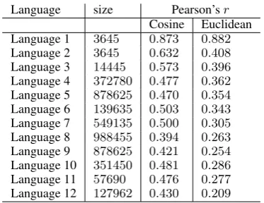
Language size Pearson’sr

Cosine Euclidean

Language 1 3645 0.873 0.882

Language 2 3645 0.632 0.408

Language 3 14445 0.573 0.396

Language 4 372780 0.477 0.362

Language 5 878625 0.470 0.354

Language 6 139635 0.503 0.343

Language 7 549135 0.500 0.305

Language 8 988455 0.394 0.263

Language 9 878625 0.421 0.254

Language 10 351450 0.481 0.286

Language 11 57690 0.476 0.277

Language 12 127962 0.430 0.209

Table 3: Correlation between embedding and distinc-tive feature space, all values significant atp <0.01

As can be noticed from the descriptions, each language defines different sets of equivalence re-lations among phones based on the contexts in which they occur. For example, in Language 3, aspirated stops occur word-initially, voiced stops occur inter-vocalically and voiceless stops occur word-finally. The task of phonology is to capture generalizations about these natural classes. No-tice that although these natural classes are based on phonetic features such as aspiration and

voic-ing, word2vec has no access to these features.

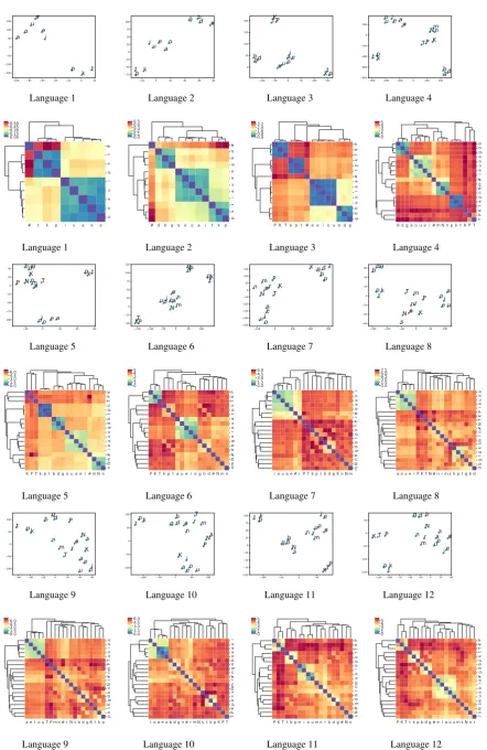
The goal of our experiments is to investigate the extent to which these natural classes can be in-ferred solely based on phone embeddings. The embedding space for each language is visualized using T-distributed Stochastic Neighbor Embed-ding (t-SNE) plots. Multiple plots were gener-ated for different values of perplexity and learn-ing rate uslearn-ing the implementation in scikit-learn toolkit (Buitinck et al.,2013). The plots shown in Figure2 correspond to perplexity 3 and learning rate100. In addition, phone clusters derived us-ing agglomerative clusterus-ing of cosine similarities between phone embeddings are also shown. Eu-clidean distance was used to plot the dendrogram heatmaps3.

From the plots, we observe that phone embed-dings capture the different context classes with varying degrees of success. Languages 1-3 were designed with unique contexts for each class of phones and the embeddings show clear separa-tion between these classes. In Language 4-5,

3_{The interpretation of these distance-based heatmaps}

dif-fers from the cosine similarity-based heatmap of Wargamay presented in the previous section.

where nasal codas are allowed, the t-SNE plot shows less separation between nasal codas and word-initial aspirated voiceless stops. This is due to the fact that in monosyllabic words, aspirated stops and nasals co-occur within the same con-text (bimoraic) window. This is an unintended co-occurrence restriction learnt by word2vec. However, this pattern in monosyllabic words has no effect on the phone clusters in the dendro-gram. Nasals and aspirated stops form separate clusters in the dendrogram. In Language 6, a co-occurrence constraint that nasal obstruent clusters be homorganic was introduced. Interestingly, the t-SNE plot for this language has nasals showing up with vowels. The syntagmatic relationship (co-occurrence restriction) between nasals and homo-organic voiced obstruents introduced in this lan-guage is not seen in the t-SNE plot of the em-bedding space. But, the dendrogram heatmap for this language shows nasals and voiced obstru-ents forming a high-level cluster. It is plausible that with hyperparameter tuning, co-occurrence restrictions such as nasal-voiced obstruent clusters are captured even in the t-SNE plots of embedding space. Co-occurrence restrictions in phonology are much more rigid than word relatedness since the size of the phone inventory in a language is many degrees smaller than the size of the vocabu-lary.

100 80 60 40 20 0 20 150 100 50 0 50 100 150 i # t ou a k e p Language 1

20 0 20 40 60 80 75 50 25 0 25 50 75 100 b i d o u a k p g e # t Language 2

100 50 0 50 100 150 0 50 100 150 200 K gbd e T u p P a kt oi # Language 3

600 400 200 0 200 400 800

600 400 200 0 200 ea

d N p P K i u g # k nm o t b T Language 4

# t k p i u a e o

# t k p i u a e o 0.00 0.15 0.30 0.45 0.60 Language 1

# d b g o e u a i t k p

# d b g o e u a i t k p 0.0 0.1 0.2 0.3 0.4 0.5 Language 2

P K T k p t # a e i o u b d g

P K T k p t # a e i o u b d g 0.0 0.8 1.6 2.4 3.2 Language 3

b d g a o u e i # m N n p k t K P T

b d g a o u ei # mN n p kt K P T 01 23 45 Language 4

20 0 20 40 60 100 75 50 25 0 25 50 g # io K d n e m kt N T u p a b P Language 5

150 100 50 0 50 100 50 25 0 25 50 75 100 125 t N P e b n i a o# g p d u k m KT Language 6

100 0 100 200 300 250 200 150 100 50 0 50 100 150 e b N T g d a P o k i u t

n #mr K p

Language 7

150 100 50 0 50 100 60 40 20 0 20 40 60 sN d r b K m k i g # t e a o p u T P n Language 8

K P T k p t b d g o u a e i # m N n

K P T k pt b d g o u a ei # mN n 0.0 1.5 3.0 4.5 6.0 Language 5

P K T k p t a u e i o g b d # N m n

P K T k pt a u ei o g b d # N mn 01 23 45 Language 6

i o u a e # r P T k p t b d g K n N m

i o u a e #r P T k pt b d g K n N m 0.0 1.5 3.0 4.5 6.0 Language 7

a o u e i P K T N # n r m s k p t g b d

a o u ei P K T N #n r ms k pt g b d 0.0 1.5 3.0 4.5 6.0 7.5 Language 8

60 40 20 0 20 40 60 100 50 0 50 100 t _k Tr oi a m # N e p P K g b u s n d Language 9

100 50 0 50 100 100 50 0 50 100 P o # m n k _g s ai p u e T N r d K b t Language 10

100 50 0 50 100 75 50 25 0 25 50 75 100 T k o t s p g m i b u P # N d e n K r Language 11

125 100 75 50 25 0 25 50 150 100 50 0 50 P o u r n e N m d i t # p s b k a g T K Language 12

a e i o u T P m n # r N s b d g K t k p

a ei o u T P mn #r Ns b d g Kt k p 0.0 1.5 3.0 4.5 6.0 Language 9

i u a e o b d g n # r mN s t k p K P T

i u a e o b d g n #r mN st k p K P T 0.0 1.5 3.0 4.5 6.0 Language 10

P K T t k p e i o u m n r b d g # N s

P K Tt k p ei o u mn r b d g # Ns 01 23 45 Language 11

P K T t k p b d g # e i a o u m s N n r

P K Tt k p b d g #e i a o u ms Nn r 01 23 45 Language 12

10-12 introduce contextual restrictions on vowels. In Language 10, only high vowels occur in the word-initial position and phone embeddings cap-ture this distinct class of vowels as shown by the dendrogram heatmap. Languages 11 and 12 show a similar pattern with respect to a different fea-ture, backness. Both of them are harmony lan-guages, which still obey the constraint that vow-els in initial syllables must be [+high]. Inter-estingly, vowels cluster with respect to [±back]

rather than[±high]as can be seen from the plots. Evidence for agreement between vowels with re-spect to backness is three times more frequent than the evidence with respect to agreement between vowels in initial syllable with respect to height. Although vowel harmony is also an instance of co-occurrence restriction (syntagmatic relationship),

word2vec infers these classes accurately. The

number of vowels in a language tends to be much lower than the number of consonants. And there-fore, it seems that a co-occurrence restriction be-tween vowels is a relatively larger sample of the set of all possible vowel sequences (5∗5∗5 = 125

in this language) compared to a co-occurrence re-striction between two or more consonants. The transparent vowelahas no effect on the distances between the other vowels in Language 12.

The ability of phone embeddings to learn phonology in our artificial language experiments can be summarized as

follows-1. Phone embeddings are able to capture paradigmatic relationships among phones very well. For example, word-initial aspi-rated stops, intervocalic voiced stops, word-final voiceless stops and vowels are recovered as separate classes in most languages.

2. Phone embeddings are also able to cap-ture positional restrictions as well as co-occurrence restrictions on vowels as shown by Languages 10-12.

3. Phone embeddings are not able to cap-ture co-occurrence restrictions among conso-nants such as homorganic nasal-voiced ob-struent clusters, voiced obob-struent-lateral clus-ter and homorganic nasal-sibilant-voiceless stop clusters. This observation is similar to one reported in the distributed semantic liter-ature that word embeddings capture similar-ity better than relatedness (Asr et al.,2018). Based on insights from the word embedding

literature, context embeddings denoted by the hidden to output layer weight matrix, are supposed to be able to capture better syn-tagmatic relationships like co-occurrence re-strictions. In addition, it is plausible that these co-occurrence restrictions among con-sonants can be learnt using autosegmental tier-based representations. We leave this in-vestigation to future work.

4 Distinctive Features and Phoneme

Induction

The main argument of this paper is that phone embeddings should be evaluated in terms of their ability to capture phonological relationships. Ap-plying this bottom-up approach to natural lan-guage phonology is not straightforward since the full set of phonological relationships is not known beforehand. Even the method of evaluating phone embeddings using the correlation between distinc-tive feature space and phone embedding space, as mentioned earlier, presupposes that the gold stan-dard specification of distinctive features for that particular language is known. However, this is sel-dom the case. Natural languages are highly com-plex with processes such as borrowing, loanword adaptation and language changes such as drift. This is why experimenting with artificial phonol-ogy can be informative.

the clusters corresponding to voiceless consonants and vowels between Language 1 and Language 12. Given the continuous space nature of phone em-beddings and the dimensionality reduction prop-erty of word2vec, this is expected. When the weights of the neural network corresponding to a particular phone or phone-sequence are adjusted, the changes affect similar items (Mikolov et al., 2013b). This inverse “dispersion” effect is also relevant to the correlation between distinctive ture space and embedding space- the value of fea-tural distance between phones is constant across languages when estimated using a fixed distinctive feature representation. But, as the number of con-text classes increases, distances between phone embeddings increase and the cumulative effect on the correlation between phonetic space and em-bedding space is downward. Thus, this correla-tion value clearly cannot be used as an evalua-tion metric for cross-linguistic comparison. Even within a language, a higher correlation value does not necessarily indicate better learning of phonol-ogy/phonetics. Rather it indicates a low inverse dispersion effect. One way to interpret the results of Silfverberg et al.(2018, pp.140) is that phone classes based on context are much less spread out in embedding space when learnt using supervised RNN compared toword2vec. At best, this can be interpreted as a difference in the dimensionality reduction properties of the two techniques.

This also raises an interesting question about the degree of specification of phones. Phonolo-gists assume a language independent feature spec-ification of phones. The results of our experiments suggest the following possibility- could the granu-larity of feature specification be dependent on how separable the different classes of phones are in em-bedding space? In other words, do learners infer distinctive features of phones based on the con-texts in which they occur? If certain phone classes can be inferred purely based on context, phonetic features that distinguish these classes can be un-derspecified. For example, in Language 10, the difference between high and non-high vowels in a language could be inferred based on context. For such a language, is it necessary to include height ([±high]) as a distinctive feature? Intuitively, the task of distinctive feature induction is related to phoneme induction.

A quantitative approach to phoneme induction based on phone embeddings and phonetic features

0.2 0.4 0.6 0.8

Phonetic distance

0.0 0.5 1.0 1.5 2.0 2.5 3.0 3.5

Contextual distance

d-o K-e

a-b

K-T K-p

a-i P-b

P-e P-i P-p

g-t d-k

e-u _p-t

t-u T-g

P-a

a-g d-t

a-t

b-e g-k

a-o

a-p

a-d T-d

P-T a-u

T-o

e-t P-t

K-P P-k

i-p T-u

o-u

p-u

d-i b-k

T-b

T-aT-i

e-p e-k g-p

b-g

i-k

a-e

K-b T-e

d-p

i-o

K-t

i-t K-o

d-u K-d

k-p K-k

P-g P-d T-p

o-p K-u

e-oi-u

g-i b-t T-t

d-g g-u

K-i

k-t b-p

b-d

b-i

e-g T-k

P-o a-k

K-a

d-e b-u

e-i

o-t K-g

k-u P-u

b-o g-o

k-o

Figure 3: Contextual distance versus Phonetic distance

p-t k-t b-d K-T b-g k-p d-g e-u e-o i-o K-P P-T a-e a-u a-o i-u a-d a-g d-e a-i o-u d-o d-u e-g a-b d-i b-o g-o b-e b-u g-u g-i a-t e-t b-i o-t t-u i-t T-a T-o o-p T-i T-e P-o p-u a-p T-u a-k e-k e-p K-a P-a P-u P-i P-e K-e i-p k-o K-o K-i i-k e-i k-u K-u g-t g-p K-d T-g K-b d-k P-g T-b b-k d-p b-t P-d K-t K-p T-k P-k P-t T-p P-b T-d K-g b-p d-t g-k P-p T-t K-k

Phone pairs

0

5

10

15

20

25

Contextual distance / Phonetic distance

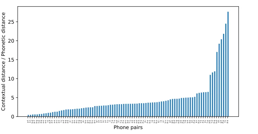
Figure 4: Allophonic index derived from embeddings

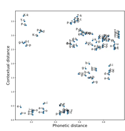
plot. The phonetic feature specifications of these pairs can be compared to discover that voicing and aspiration are not phonemic in this language. Sim-ilarly, phone pairs that show up at the bottom left corner of this plot such as the 10 pairs of vow-els and P-T, P-K, K-T, p-t, t-k, p-k, b-d, d-g andg-bare all phonemic contrasts. The phonetic specifications of these phone pairs can be com-pared to discover that both height and backness are contrastive for vowels and place of articulation is contrastive for consonants. The remaining phone pairs in the top right corner of the scatter plot are all phonemic contrasts. However, they might not yield any new distinctive features. The bar plot in Figure4is another way of visualizing the use-fulness of distances between phone embeddings to identify phonemic versus allophonic relationships. We define allophonic index as the ratio of contex-tual distance estimated using phone embeddings to phonetic distance. The higher the value of this index for a phone pair, the more likely the pair is to be allophonic. The sorted bar plot in Fig-ure4corresponding to artificial Language 3 shows allophonic pairs at the right edge and phonemic pairs at the left edge. A precise formulation of a phoneme/distinctive feature induction algorithm based on these metrics is reserved for future work.

5 Conclusions and Future work

This paper presents a discussion of evaluation of phone embeddings. Artificial language

experi-ments are used to study word2vec’s ability to learn different kinds of phonological relationships. The results show that phone embeddings are able to capture phonemic and allophonic relationships quite well. Phone embeddings are also able to capture co-occurrence restrictions among vowels found in harmony languages. Phone embeddings do not perform well on capturing co-occurrence restrictions among consonants. The experimen-tal results also show an interesting correlation be-tween size and complexity of phone inventory and magnitude of inter-phone distances based on phone embeddings. An analysis of the limitation of correlation between embedding space and dis-tinctive feature space to evaluate phone embed-dings for their learning of phonology is also pro-vided. The analytical framework presented here and the proposal for distinctive feature induction will be developed in future work and can be ap-plied to diverse problems ranging from bootstrap-ping pronunciations of OOV words in ASR to modeling historical phonology. A similar analysis of sound analogies is required to better understand their significance to phonology.

6 Acknowledgements

References

Fatemeh Torabi Asr and Michael Jones. 2017.An arti-ficial language evaluation of distributional semantic models. InProceedings of the 21st Conference on Computational Natural Language Learning (CoNLL 2017), pages 134–142. Association for Computa-tional Linguistics.

Fatemeh Torabi Asr, Robert Zinkov, and Michael

Jones. 2018. Querying word embeddings for

sim-ilarity and relatedness. InProceedings of the 2018 Conference of the North American Chapter of the Association for Computational Linguistics: Human Language Technologies, Volume 1 (Long Papers), pages 675–684. Association for Computational Lin-guistics.

Marco Baroni, Georgiana Dinu, and Germ´an

Kruszewski. 2014. Don’t count, predict! a

systematic comparison of context-counting vs. context-predicting semantic vectors. InProceedings of the 52nd Annual Meeting of the Association for Computational Linguistics (Volume 1: Long Papers), pages 238–247. Association for Computa-tional Linguistics.

Lars Buitinck, Gilles Louppe, Mathieu Blondel, Fabian Pedregosa, Andreas Mueller, Olivier Grisel, Vlad Niculae, Peter Prettenhofer, Alexandre Gramfort, Jaques Grobler, Robert Layton, Jake VanderPlas, Arnaud Joly, Brian Holt, and Ga¨el Varoquaux. 2013. API design for machine learning software: experi-ences from the scikit-learn project. InECML PKDD Workshop: Languages for Data Mining and Ma-chine Learning, pages 108–122.

Bruce Hayes and Colin Wilson. 2008. A maximum en-tropy model of phonotactics and phonotactic learn-ing. Linguistic inquiry, 39(3):379–440.

Roman Jakobson, C Gunnar Fant, and Morris Halle. 1951. Preliminaries to speech analysis: The dis-tinctive features and their correlates. MIT press. Peter Ladefoged and Keith Johnson. 2010.A course in

Phonetics. Thomson Wadsworth Boston.

Omer Levy, Yoav Goldberg, and Ido Dagan. 2015. Im-proving distributional similarity with lessons learned from word embeddings.Transactions of the Associ-ation for ComputAssoci-ational Linguistics, 3:211–225. Tomas Mikolov, Kai Chen, Greg Corrado, and

Jef-frey Dean. 2013a. Efficient estimation of word

representations in vector space. arXiv preprint arXiv:1301.3781.

Tomas Mikolov, Wen-tau Yih, and Geoffrey Zweig. 2013b. Linguistic regularities in continuous space word representations. In Proceedings of the 2013 Conference of the North American Chapter of the Association for Computational Linguistics: Human Language Technologies, pages 746–751.

Allison Parrish. 2017. Poetic sound similarity vec-tors using phonetic features. In Thirteenth Artifi-cial Intelligence and Interactive Digital Entertain-ment Conference.

Jeffrey Pennington, Richard Socher, and Christopher

Manning. 2014. Glove: Global vectors for word

representation. In Proceedings of the 2014 Con-ference on Empirical Methods in Natural Language Processing (EMNLP), pages 1532–1543. Associa-tion for ComputaAssocia-tional Linguistics.

Radim ˇReh˚uˇrek and Petr Sojka. 2010. Software Frame-work for Topic Modelling with Large Corpora. In Proceedings of the LREC 2010 Workshop on New Challenges for NLP Frameworks, pages 45–50,

Val-letta, Malta. ELRA. http://is.muni.cz/

publication/884893/en.

Miikka P Silfverberg, Lingshuang Mao, and Mans Hulden. 2018. Sound analogies with phoneme em-beddings. Proceedings of the Society for Computa-tion in Linguistics (SCiL) 2018, pages 136–144. Pavel Sofroniev and C¸ a˘grı C¸ ¨oltekin. 2018. Phonetic