Optimal measurements for simultaneous quantum estimation of multiple phases

(1)

warwick.ac.uk/lib-publications

Original citation:

Pezzè, Luca, Ciampini, Mario A., Spagnolo, Nicolò, Humphreys, Peter C., Datta, Animesh,

Walmsley, Ian A., Barbieri, Marco, Sciarrino, Fabio and Smerzi, Augusto (2017) Optimal

measurements for simultaneous quantum estimation of multiple phases. Physical Review

Letters, 119 (13). 130504. doi:10.1103/PhysRevLett.119.130504

Permanent WRAP URL:

http://wrap.warwick.ac.uk/98200

Copyright and reuse:

The Warwick Research Archive Portal (WRAP) makes this work by researchers of the

University of Warwick available open access under the following conditions. Copyright ©

and all moral rights to the version of the paper presented here belong to the individual

author(s) and/or other copyright owners. To the extent reasonable and practicable the

material made available in WRAP has been checked for eligibility before being made

available.

Copies of full items can be used for personal research or study, educational, or not-for-profit

purposes without prior permission or charge. Provided that the authors, title and full

bibliographic details are credited, a hyperlink and/or URL is given for the original metadata

page and the content is not changed in any way.

Publisher statement:

© 2017 American Physical Society

A note on versions:

The version presented here may differ from the published version or, version of record, if

you wish to cite this item you are advised to consult the publisher’s version. Please see the

‘permanent WRAP URL’ above for details on accessing the published version and note that

access may require a subscription.

(2)

Optimal measurements for simultaneous quantum estimation of multiple phases

Luca Pezz`e,1 Mario A. Ciampini,2 Nicol`o Spagnolo,2 Peter C. Humphreys,3 Animesh Datta,4 _{Ian A. Walmsley,}3 _{Marco Barbieri,}5 _{Fabio Sciarrino,}2 _{and Augusto Smerzi}1

1_{QSTAR, INO-CNR and LENS, Largo Enrico Fermi 2, I-50125 Firenze, Italy} 2

Dipartimento di Fisica, Sapienza Universit`a di Roma, Piazzale Aldo Moro 5, I-00185 Roma, Italy 3

Department of Physics, Clarendon Laboratory, University of Oxford, Oxford OX1 3PU, United Kingdom 4_{Department of Physics, University of Warwick, Coventry CV4 7AL, United Kingdom}

5

Dipartimento di Scienze, Universit`a degli Studi Roma Tre, Via della Vasca Navale 84, 00146, Rome, Italy

(Dated: May 11, 2017)

A quantum theory of multiphase estimation is crucial for quantum-enhanced sensing and imag-ing and may link quantum metrology to more complex quantum computation and communication protocols. In this letter we tackle one of the key difficulties of multiphase estimation: obtaining a measurement which saturates the fundamental sensitivity bounds. We derive necessary and sufficient conditions for projective measurements acting on pure states to saturate the maximal theoretical bound on precision given by the quantum Fisher information matrix. We apply our theory to the specific example of interferometric phase estimation using photon number measurements, a conve-nient choice in the laboratory. Our results thus introduce concepts and methods relevant to the future theoretical and experimental development of multiparameter estimation.

Introduction. Quantum metrology is currently attract-ing considerable interest in the light of its technological applications. Theoretical developments and experimen-tal investigations have, so far, mostly focussed on the estimation of single phase [1–3], for which the ultimate sensitivity bounds and explicit conditions for their sat-uration are well known [4, 5]. These studies have been further extended in order to understand the connection between enhancement in phase estimation and particle entanglement [6–9], as well as the impact of noise and dissipation on the fundamental bounds [10, 11]. Several proof-of-principle experiments have demonstrated phase estimation below the classical (shot-noise) limit [2], in-cluding applications in fields as diverse as magnetometry [12], atomic clocks [13] and optical detection of gravita-tional waves [14].

Yet, a significant class of problems can not be effi-ciently cast as the estimation of a single parameter, as is the case for quantum sensing and imaging [15], and for quantum communication and computation protocols [16, 17]. Such multiparameter cases have been the sub-ject of recent efforts, investigating the role of entan-glement [18], and the impact of noise and decoherence [19, 20]. Explicit examples have been considered, includ-ing measurement strategies for state estimation [21, 22], the joint estimation of phase and loss rate [23, 24], phase and phase diffusion [25–28], components of a displace-ment in phase space [29, 30], multiple phases [18, 31], parameters belonging to multidimensional fields [32], and estimation tasks with partial knowledge on the actual measurement device [33].

However, there are still several open questions in multi-parameter estimation, one of the most urgent of which is to find saturable lower bounds of phase sensitivity. There exists a fundamental bound – the quantum Cramer-Rao bound – which has been formulated in [34] for the multi-parameter case. However, unlike in the single-multi-parameter case, the quantum Cram´er-Rao bound is not always

sat-urable, with a necessary condition provided by the com-mutativity of the symmetric logarithmic derivatives. Fur-thermore, it does not provide a recipe for constructing optimal measurements [3, 31, 34, 36, 37].

In this manuscript, we discuss the properties that a projective measurement must have in order to saturate the quantum Cramer-Rao bound for multiphase estima-tion with probe pure states. Our results extend and com-plement previous works by Helstrom [34], Matsumoto [36], and Humphreys et al. [31], by identifying the nec-essary and sufficient conditions on the projectors. Dif-ferently from earlier investigations, we do not focus on specific instances, but provide general constructive con-ditions for obtaining an optimal measurement not limited by non-commutativity. This has implications for the fu-ture experimental and theoretical development of multi-phase estimation with quantum technologies, including photons, atoms and trapped ions.

Multiphase estimation. The simultaneous estimation of ad-dimensional vector parameter θ ={θ1, θ2, ..., θd}

[image:2.612.321.568.551.644.2]

measurement estimator probe state evolution

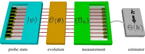
Figure 1: General framework of multiparameter estimation considered in this manuscript: a probe state|ψiis prepared, transformed according to the unitary parameter-dependent transformation ˆU(θ) and measured by a set of projectors

{_Πkˆ _}_{. The value of the vector parameter is retrieved via an} estimator Θ(k), function of the measurement outcomes.

(3)

follows the standard steps of quantum metrology (see Fig. 1): (i)A probe state is prepared (here we will consider a pure probe state|ψi). (ii)It is shifted in phase by ap-plying a phase-encoding unitary transformation ˆUθ, the

output state being|ψsi ≡Uˆθ|ψi. (iii) The output state

is detected. In the following we will consider a set of projective measurements {Πkˆ }k, labelled by the indexk

representing the possible result. Eventually, the proto-col is repeated ν times using independent and identical copies of the output state (with the same transforma-tion and output measurement). (iv) Finally, from the output results k ≡ {k1, ..., kν} one infers the vector pa-rameter via a suitably chosen function Θ(k), called the estimator. The probability of observing the sequence

k, conditioned to the vector parameter θ, is given by

P(k|θ) =Qν

i=1P(ki|θ) andP(k|θ) =hψs|Πkˆ |ψsi. In the following we will consider locally unbiased estimators, for which the average value of the estimator equals the true value of the parameter: ¯Θ(k) =P

kP(k|θ)Θ(k) =θand dΘ(¯ k)/dθl = 1 (l = 1, ..., d). A figure of merit of phase sensitivity is the covariance matrix,

[B(θ)]l,m=X

k

P(k|θ) ¯θ−θ

l θ¯−θ

m. (S.1)

The diagonal elements Bl,l equal the variance (∆θl)2. For any unbiased estimators, and independent measure-ments, the chain of inequalities

B(θ)≥ [F(θ)]

−1

ν ≥

[FQ(θ)]−1

ν (S.2)

holds (in the matrix sense). The first inequality is the Cramer-Rao bound, where

[F(θ)]l,m=

X

k

∂lP(k|θ)∂mP(k|θ)

P(k|θ) (S.3)

is thed×dsymmetric Fisher information matrix (FIM), and ∂l = ∂/∂θl. Since ∂lP(k|θ) = 2Re[h∂lψs|Πkˆ |ψsi], the FIM depends on how the measurement set acts on the Hilbert subspaceHspanned by the probe state|ψsi and {|∂lψsi}l=1,...,d. Here Re[x] and Im[x] indicate the

real and imaginary part ofx, respectively, and |∂lψsi=

−iHˆl|ψsi, where ˆHl≡i[∂lUˆ(θ)] ˆU†(θ) is a Hermitian op-erator. The Cramer-Rao bound can be established only if the FIM is strictly positive (and thus invertible). In this case, it can always be saturated, asymptotically in

ν, by the maximum likelihood estimator [34]. The sec-ond bound in Eq. (S.2) is due to F(θ) ≤ FQ(θ) [34], where FQ(θ) is the quantum Fisher information matrix (QFIM),

[FQ(θ)]l,m= 4Re[h∂lψs|∂mψsi] + 4h∂lψs|ψsih∂mψs|ψsi. (S.4) We recall that the inequality F ≤FQ is understood in

the matrix sense, i.e. u>F u≤ u>FQu holds for arbi-trary d-dimensional real vectors u. The inverse of the QFIM – when it exists – sets a lower bound (S.2) for the

simultaneous estimation of multiple parameters, called the quantum Cramer-Rao bound, which only depends on the probe state and phase encoding transformation. The QFIM is a particularly appealing quantity: it is propor-tional to the second-order Taylor expansion of the multi-dimensional Bures distance and, equivalently, the square root of the fidelity between quantum states [4]. It is a quantum statistical speed quantifying how much the out-put state differs from the inout-put one when applying small phase shifts [8, 35]. There is a major problem though: while in the single parameter case it is always possible to choose an optimal measurement for which the equality

F=FQ holds [4, 5], in the multiparameter case (d >1) such an optimal measurement does not exist in general.

The search for conditions under which the FIM sat-urates the QFIM has long engaged the field of quan-tum metrology [34, 36]. For non-commuting operators the main result available in the literature is due to Mat-sumoto [36]:

Weak commutativity theorem (Matsumoto). Given the pure state |ψsi, it is possible to saturate the equality

F(θ)=FQ(θ) if and only if

Im[h∂lψs|∂mψsi] = 0, ∀l, m. (S.5)

To be more precise, the condition (S.5) is necessary and, if Eq. (S.5) holds and the QFIM is invertible, Mat-sumoto proved that it is possible to constructs a set of projectors for which F(θ)=FQ(θ) holds [36]. Note that, for unitary transformations, Eq. (S.5) becomes

hψs|[ ˆHl,Hˆm]|ψsi = 0. Therefore, the (strong) com-mutativity condition [ ˆHl,Hˆm] = 0 for all l, m, implies Eq. (S.5), while the saturationF(θ)=FQ(θ) is also pos-sible for non-commuting generators [32, 36].

Generally speaking, an experimental apparatus is set by a specific probe state, transformation and (projective) measurements and it would be highly desirable to know whether – within the specific setup – it is possible to sat-urate the QFIM. To this end, the weak commutativity theorem is of little practical use: it only provides spe-cific measurements for whichF=FQholds that, however,

might not be those implemented experimentally. The sat-uration of the QFIM in an actual experiment is thus an open question in the literature, even for pure states and under the condition [ ˆHl,Hˆm] = 0 for alll, m.

In the following we provide three theorems giving nec-essary and sufficient conditions on projective measure-ments to saturateF=FQfor arbitrary generator of phase encoding (without assuming thatF_Q−1exists). It is worth pointing out that if the FIM is invertible, then our con-ditions become necessary and sufficient to saturate the quantum Cramer-Rao bound with projective measure-ments. We discuss the main consequences of our findings and the relation with existing results. The proof of the theorems is detailed in appendix:

(4)

3

fork= 1) and on the orthogonal subspace (hΥk|ψsi= 0, fork6= 1), the equalityF(θ)=FQ(θ) holds if and only if

lim

ϕ→θ

Im[h∂lψϕ|ΥkihΥk|ψϕi]

|hΥk|ψϕi|

= 0, (S.6)

for alll= 1,2, ..., dand allk6= 1.

It is possible to demonstrate that Eq. (S.6) is consis-tent with the weak commutativity condition (S.5), see appendix. In the single parameter case, where U(θ) =

e−iHθˆ and ˆH is a Hermitian operator, Eq. (S.6) is always satisfied: it is thus always possible to saturate the QFI by taking a measurement set made by the projector on the probe state|ψsiand any set of projectors on the orthog-onal subspace. In general, this measurement is different from the set of projectors on the eigenstates of the sym-metric logarithmic derivative (SLD), which also saturates the quantum Fisher information [4]. In Ref. [31] it has been claimed that any projective measurement orthogo-nal to the probe state saturates the QFIM in the multi parameter case (d >1). We emphasize that only the or-thogonal projective measurements which satisfy Eq. (S.6) saturate the QFIM. The condition (S.6) is highly nontriv-ial: it is easy to find examples of projective measurements that do not fulfill Eq. (S.6), and for whichF(θ)6=FQ(θ):

an experimentally relevant example is discussed below. If we assume that hΥk|∂jψsi= 0 does not hold for all

j = 1, ..., d, then [calculating the limit (S.6), under the conditions of Theorem #1]F(θ) =FQ(θ) if and only if

Im

h∂lψs|ΥkihΥk|∂mψsi

= 0, (S.7)

for all indicesl, m= 1,2, ..., dand allk. IfhΥk|∂jψsi= 0 for allj= 1, ..., dthen it is possible to find necessary and sufficient conditions similar to Eq. (S.7) and involving higher order derivatives. A consequence of the above theorem is the following:

Corollary #1. Given a probe pure state and

uni-tary transformations, it is always possible to saturate

F(θ)=FQ(θ) by a set of projectors given by the probe state itself and a suitable choice of vectors on the orthog-onal subspace.

Here we explicitly construct optimal projectors satu-rating the QFIM. We recall that the FIM atθ depends only on|ψsiand thedvectors{|∂mψsi}m=1,...,d. In

gen-eral, the states|∂mψsiare not orthogonal to the probe. To construct a set of projectors orthogonal to |ψsi, we introduce the set of states

|ωmi ≡ |∂mψsi+|ψsih∂mψs|ψsi, (S.8)

for m = 1, ..., d. These satisfy hψs|ωmi = 2Re[h∂mψs|ψsi] =∂mhψs|ψsi= 0 [38]. The states (S.8) are not orthogonal to each others, in general, and we can introduce thed×dGram matrixΩl,m=hωl|ωmi=

h∂lψs|∂mψsi+h∂lψs|ψsih∂mψs|ψsi. It should be noticed that, according to Eq. (S.5), the saturation of the QFIM requires Im[Ω] = Im[h∂lψs|∂mψsi] = 0. We thus neces-sarily restrict to matricesΩthat are real and symmetric.

In particular, FQ = 4Ω, see Eq. (S.4), and the QFIM is positive definite (and thus invertible) if and only if the vectors (S.8) are linearly independent. We can con-struct, via the Gram-Schmidt process, for instance, an orthogonal basis of the subspace H \ |ψsihψs| as linear combinations of states (S.8)

|Υki= d

X

m=1

bm,k|ωmi, (S.9)

with real coefficientsbm,k. With this choice, Eq. (S.7) is satisfied by the constructed set{|Υki}since

h∂lψs|Υki= d

X

m=1

Ωl,mbm,k (S.10)

is real. This concludes the proof of the corollary. The projectors of Theorem #1 constitute a limited set: from an experimental perspective, a set of projec-tors orthogonal to a given probe state may not be easily available. In this respect, it is this interesting to derive statements for more general projectors. We have:

Theorem 2 (Projective measurement not or-thogonal to the probe): Let us consider a probe pure state |ψsi and a set of projectors {|ΥkihΥk|}k not or-thogonal to the probe (i.e. hΥk|ψsi 6= 0 for all k). The equalityF(θ)=FQ(θ) holds if and only if

Im[h∂lψs|ΥkihΥk|ψsi] =|hψs|Υki|2Im[h∂lψs|ψsi], (S.11) for alll= 1,2, ..., dand allk.

In the single parameter case, Eq. (S.11) becomes Re[hψs|Hˆ|ΥkihΥk|ψsi] = |hψs|Υki|2hψs|Hˆ|ψsi, for all Υk. This is precisely the necessary and sufficient con-ditions given in Ref. [39] for the saturation of the quan-tum Fisher information for the single parameter. It is also possible to demonstrate that Eq. (S.11) implies the weak commutativity condition (S.5), see appendix for a demonstration. Similarly as above we have:

Corollary #2. Given a pure probe state and

uni-tary transformations, there always exists a set of pro-jectors non orthogonal to the probe which saturates

F(θ)=FQ(θ).

We prove the corollary by constructing a set of projec-tors that satisfy Eq. (S.11). Restricting to the subspace

H, we can decompose the states|Υki in the basis given by|ψsiand{|∂mψsi}m=1,...,d. We take

|Υki= d

X

m=1

bm,k|ωmi+bd+1,k|ψsi, (S.12)

where|ωniis given in Eq. (S.8) and we require bd+1,k =

hψs|Υki 6= 0 for all k. Equation (S.11) is fulfilled by taking real bm,k (for m = 1,2, ..., d+ 1) and noticing thath∂lψs|ωniis necessarily real to fulfill Eq. (S.5) [40]. The real coefficients in Eq. (S.12) must be chosen such thatP

(5)

all these conditions can be constructed via the Gram-Schmidt process.

Finally, it is possible to combine the results of the two theorems and corollaries discussed above and extend the saturation condition to an arbitrary set of projectors with elements that may be either orthogonal or not to the probe:

Theorem 3 (General projective measurement):

Consider a probe pure state |ψsi and a set of projec-tors {|ΥkihΥk|}k. The equality F(θ)=FQ(θ) holds if and only if Eq. (S.6) is fulfilled for all indicesl, mand all

kfor whichhΥk|ψsi= 0, and Eq. (S.11) is fulfilled for all indicesl and allkfor whichhΥk|ψsi 6= 0.

Corollary #3. Given a pure probe state and unitary transformations, it is always possible to find a set of projectors satisfying the theorem #3 and thus saturate

F(θ)=FQ(θ).

The proof of this statement immediately follows from Corollary #2 by taking real coefficients bm,k (for m = 1, ..., d), andbd+1,keither real and finite, or equal to zero. We point out that the projective measurement previously constructed by Matsumoto [36] to saturated the equality

F(θ)=FQ(θ) explicitly requires FQ(θ) to be invertible, a condition which is not general and not required in our case. It is possible to show that the specific class of pro-jective measurement used in the proof of the weak com-mutativity theorem satisfies the conditions of Theorem #3.

Examples. Generally, optical and atomic

interferome-Figure 2: ||F −FQ||2 of a three-mode (a) and a four-mode

(b) interferometer (see text and appendix) for the estimation ofθ= (θ1, θ2). For the three-mode interferometer, there is no

value ofθwhere the theorems are satisfied. Consistently, we find||F−FQ||2>3/4. For the four-mode interferometer, we

can find values ofθwhere the saturation conditionsF =FQ discussed in the manuscript are fulfilled: these are given by the dashed line and circles.

ters use the measurement of the number of particles at the output ports in order to estimate the parameter(s). Number counting realizes a projective measurement. Us-ing our results it is thus possible to tell whether or not, given a probe pure state and a phase encoding transfor-mation, the FIM obtained with number counting satu-rates the QFIM. Let us consider an-mode Mach-Zehnder interferometer (MZI), which is a generalized version – withnarms – of the common two-mode MZI [1, 2]. This apparatus allows the simultaneous estimation of multi-ple (up ton−1) phases. Three- and four-mode (MZIs) are currently within reach of present technology [41–43]. We first discuss the three-mode case with a Fock state

|ψi= |1,1,1ias input. The initial step of the interfer-ometer is a three-mode splitter, a tritter, described by the unitary matrix U_j,k(3) = 3−1/2_ei2π/3(1−δj,k)_{. Two}

op-tical phasesθ1 and θ2 are inserted in two of the modes

of the interferometer and are the parameters to be esti-mated simultaneously. After phase encoding, the mode recombine at a second three-mode splitter, described by a unitary matrix [U(3)_]−1_{. Finally, photons in each mode}

are counted. This measurement corresponds to a pro-jection over all the possible states |Υki = |i, j, hi with

i+j+h= 3. We test the conditions (S.6) and (S.11) for different values of θ = (θ1, θ2). In particular, for θ= (0,0), we have a projection over the probe state and over the orthogonal subspace. We find that the condi-tion (S.6) and (S.11) are not fulfilled. In Fig. 2(a) we plot ||F −FQ||2 by varying θ (the norm ||F −FQ||2

ranges from 0 to ||FQ||2 that is equal to 8 in this case.

We find that||F−FQ||2>0 (||F−FQ||2>3/4, in

par-ticular), consistent with the prediction of our theorems. We have repeated the analysis for a four-mode interfer-ometer, consisting of two cascaded quarters, in which a four photon|1,1,1,1iFock state is injected. The quar-ters are optical devices represented by the unitary matrix

U_j,k(4) = 2−1₍₋₁₎1−δj,k_{. Again we consider the estimation}

of two phase and choose photon counting as measure-ment method. In this case, for certain values of θ the conditions (S.6) and (S.11) are fulfilled and the QFIM is saturated for the estimation of the two phases simul-taneously: these are the values θ1 =θ2 [dashed line in

Fig. 2(b)], and the pointsθ= (0, π) andθ = (π,0) (cir-cles). Consistently, we find that||F−FQ||2= 0 for these

values ofθ.

[image:5.612.59.277.418.622.2]

(6)

5

Cramer-Rao bound when the quantum Fisher informa-tion matrix is invertible. Our results are a step forward to the theoretical understanding of multiparameter esti-mation: the ability to saturate the QFIM is a key for the experimental design of future quantum imaging and multiparameter metrology devices.

Acknowledgements. M.B. is supported by a Rita Levi-Montalcini fellowship of MIUR. This work was sup-ported by the ERC-Starting Grant 3D-QUEST

(3D-Quantum Integrated Optical Simulation; grant agree-ment no. 307783): http://www.3dquest.eu, and by the H2020-FETPROACT-2014 Grant QUCHIP (Quantum Simulation on a Photonic Chip; grant agreement no. 641039): http://www.quchip.eu. AD is supported by the UK EPSRC (EP/K04057X/2) and the UK National Quantum Technologies Programme (EP/M01326X/1, EP/M013243/1).

[1] V. Giovannetti and S. Lloyd and L. Maccone,Nat. Phot.

5, 222 (2011).

[2] L. Pezz`e, A. Smerzi, M.K. Oberthaler, R. Schmied and P. Treutlein, arXiv:1609.01609.

[3] M.G.A. Paris,Int. J. Quantum Inform.7, 125 (2009). [4] S.L. Braunstein and C.M. Caves, Phys. Rev. Lett. 72,

3439 (1994).

[5] S.L. Braunstein, C.M. Caves and G.J. Milburn, Ann. Phys.247, 135 (1996).

[6] L. Pezz`e and A. Smerzi, Phys. Rev. Lett. 102, 100401 (2009).

[7] P. Hyllus, et al., Phys. Rev. A 85, 022321 (2012); G. T`oth,Phys. Rev. A85, 022322 (2012).

[8] L. Pezz`e, Y. Li, W. Li, and A. Smerzi,PNAS113, 11459 (2016).

[9] V. Giovannetti and S. Lloyd and L. Maccone,Phys. Rev. Lett.96, 010401 (2006).

[10] R. Demkowicz-Dobrzanski, J. Kolodynski and M. Guta,

Nat. Comm.3, 1063 (2012).

[11] B. M. Escher, R. L. de Matos Filho and L. Davidovich,

Nat. Phys.7, 406 (2011).

[12] R. J. Sewell, M. Koschorreck, M. Napolitano, B. Dubost, N. Behbood, and M. W. Mitchell,Phys. Rev. Lett.109, 253605 (2012); C.F. Ockeloen, R. Schmied, M.F. Riedel, and P. Treutlein, Phys. Rev. Lett. 111, 143001 (2013); W. Muessel, H. Strobel, D. Linnemann, D.B. Hume, and M. K. Oberthaler,Phys. Rev. Lett.113, 103004 (2014). [13] A. Louchet-Chauvet, J. Appel, J.J. Renema, D. Oblak,

N. Kjrgaard, and E. S. Polzik,New J. Phys. 12, 065032 (2010); I. D. Leroux, M.H. Schleier-Smith, and V. Vuletic,Phys. Rev. Lett.104, 250801 (2010); O. Hosten, N. J. Engelsen, R. Krishnakumar, and M. A. Kasevich,

Nature529, 505 (2016); I. Kruse, et al.,Phys. Rev. Lett.

117, 143004 (2016).

[14] The LIGO Scientific Collaboration,Nat. Phys.7, 962-965 (2011).

[15] C. Preza, D. L. Snyder, and J. A. Conchello,J. Opt. Soc. Am. A16, 2185 (1999).

[16] C. E. Granade, C. Ferrie, N. Wiebe, and D. G. Cory,New J. Phys. 14, 103013 (2012).

[17] F. Huszar and N. M. T. Houlsby,Phys. Rev. A85, 052120 (2012).

[18] M.A. Ciampini, N. Spagnolo, C. Vitelli, L. Pezz`e, A. Smerzi and F. Sciarrino,Sci. Rep.6, 28881 (2016). [19] J.-D. Yue, Y.-R. Zhang and H. Fan, Sci. Rep. 4, 5933

(2014).

[20] P. A. Knott, T. J. Proctor, A. J. Hayes, J. F. Ralph, P. Kok, and J. A. Dunningham, Phys. Rev. A 94, 062312 (2016)

[21] R. D. Gill and S. Massar,Phys. Rev. A61, 042312 (2000).

[22] N. Li, C. Ferrie, J. A. Gross, A. Kalev, and C. M. Caves,

Phys. Rev. Lett.116, 180402 (2016).

[23] O. Pinel, P. Jian, N. Treps, C. Fabre, and D. Braun,

Phys. Rev A88040102(R) (2013).

[24] P.J.D. Crowley, A. Datta, M. Barbieri, and I.A. Walms-ley,Phys. Rev. A89, 023845 (2014).

[25] M.D. Vidrighin, G. Donati, M.G. Genoni, X-M. Jin, W.S Kolthammer, M.S. Kim, A. Datta, M. Barbieri and I.A. Walmsley,Nat. Comm.5, 3532 (2014).

[26] S.I. Knysh, and G.A. Durkin, arXiv:1307.0470 (2013). [27] M. Altorioet al.,Phys. Rev. A92, 032114 (2015). [28] M. Szczykulska, T. Baumgratz, and A. Datta,

arXiv:1701.07520 (2017).

[29] M.G. Genoni, M.G.A. Paris, G. Adesso, H. Nha, P.L. Knight, and M.S. KimPhys. Rev. A87, 012107 (2013). [30] S. Steinlechneret al. Nature Photon.7, 626 (2013). [31] P.C. Humphreys, M. Barbieri, A. Datta and I.A.

Walm-sley,Phys. Rev. Lett.111, 070403 (2013).

[32] T. Baumgratz and A. Datta,Phys Rev. Lett.116, 030801 (2016).

[33] M. Altorioet al.,Phys. Rev. Lett.116, 100802 (2016). [34] C.W. Helstrom, Quantum Detection and Estimation

Theory(Academic, 1976).

[35] H. Strobel,et al.,Science345, 424 (2014). [36] K. Matsumoto,J. Phys. A35, 3111 (2002).

[37] S. Ragy, M. Jarzyna, and R. Demkowicz-Dobrza´nski,

Phys. Rev. A94, 052108 (2016).

|ψsihψs|Lˆm. We have 4Re[hωl|ωmi] = [FQ]l,m.

[39] T. Wasak, J. Chwedenczuk, L. Pezz`e, A. Smerzi,Quant. Inf. Proc.1-22 (2016).

[40] We have hψs|Υki = bd+1,k and h∂lψs|Υki =

Pd

m=1bm,kh∂lψs|ωmi + bd+1,kh∂lψs|ψsi. If

we take real coefficients cm,k (with m = 1,2, ..., d + 1), we find Im[h∂lψs|ΥkihΥk|ψsi] =

|hψs|Υki|2Im[h∂lψs|ψsi], which is exactly Eq. (S.11). [41] N. Spagnolo, L. Aparo, C. Vitelli, A. Crespi, R. Ramponi,

R. Osellame, P. Mataloni, and F. Sciarrino,Sci. Rep.2, 862 (2012).

[42] N. Spagnolo, C. Vitelli, L. Aparo, P. Mataloni, F. Sciar-rino, A. Crespi, R. Ramponi and R. Osellame,Nat. Com-mun.4, 1606 (2013).

(7)

Appendix A: Proof of theorem #1.

Let us consider a projective set {|ΥkihΥk|}k where the element k = 1 is the projection over the probe state

hΥk|ψsi= 0 for allk6= 1. From Eq. (3), the FIM atθ is given by

[F(θ)]l,m= lim

ϕ→θ[F(ϕ)]l,m, (S.1)

where

[F(ϕ)]l,m= 4

Re[h∂lψϕ|ψsihψs|ψϕi] Re[h∂mψϕ|ψsihψs|ψϕi]

|hψs|ψϕi|2

+ 4X k6=1

Re[h∂lψϕ|ΥkihΥk|ψϕi] Re[h∂mψϕ|ΥkihΥk|ψϕi]

|hΥk|ψϕi|2

.

[F(θ)]l,m= 4 lim

ϕ→θ

X

k6=1

Re[h∂lψϕ|ΥkihΥk|ψϕi] Re[h∂mψϕ|ΥkihΥk|ψϕi]

|hΥk|ψϕi|2

. (S.3)

This limit is undetermined (0/0). In the following we demonstrate that the inequality F(θ)≤FQ(θ) holds and find the necessary and sufficient condition for the saturation of the equality sign. From Eq. (S.3) we have

uTF(θ)u= d

X

l,m=1

ul[F(θ)]l,mum= 4 lim

ϕ→θ

X

k6=1

Re[hΨu|ΥkihΥk|ψϕi]

2

|hΥk|ψϕi|2

, (S.4)

where |Ψui ≡P

d

l=1ul|∂lψϕi. We now use Re[x]2 =|x|2−Im[x]2. In particular,|hΨu|ΥkihΥk|ψϕi|2/|hΥk|ψϕi|2 =

|hΨu|Υki|2. We thus find

uTF(θ)u = 4 lim

ϕ→θ

X

k6=1

|hΨu|Υki|2−4 lim

ϕ→θ

X

k6=1

Im[hΨu|ΥkihΥk|ψϕi]

2

|hΥk|ψϕi|2

, (S.5)

= uTFQ(θ)u−4 lim ϕ→θ

X

k6=1

Im[hΨu|ΥkihΥk|ψϕi]

2

|hΥk|ψϕi|2

. (S.6)

1− |ψsihψs|. The second term in Eq. (S.6) is always positive and bounded byuTFQ(θ)u. Therefore,F(θ)≤FQ(θ), as expected, with equality if and only if the second term in Eq. (S.6) vanishes. Since this is given by a sum (over

k6= 1) of positive terms, the equality is obtained if and only if each term of the sum vanishes for an arbitrary choice ofu. We thus conclude thatF(θ) =FQ(θ) holds if and only if

lim

ϕ→θ

|hΥk|ψϕi|

= 0, ∀l, and∀k6= 1. (S.7)

This is our most general condition and coincides with Eq. (6) of the main paper. The limit in Eq. (S.7) is undetermined (0/0) and to calculate it we proceed with a Taylor expansion of|ψϕiand|∂lψϕi. To the leading order inδϕ=ϕ−θ,

we have

|hΥk|ψϕi|

=

Pd

j=1Im[h∂lψs|ΥkihΥk|∂jψsi]δϕj+O(δϕ2)

|Pd

j=1hΥk|∂jψsiδϕj+O(δϕ2)|

. (S.8)

Excluding the casehΥk|∂jψsi= 0 for allj, the limit exists and it is equal to zero if and only if

Imh∂lψs|ΥkihΥk|∂mψsi

= 0, ∀l, m, ∀k6= 1. (S.9)

(8)

7

1. Consistency with Matsumoto’s condition

Here we show that Eq. (S.7) implies Matsumoto’s weak commutativity condition Im[h∂lψs|∂mψsi] = 0 for all

l, m= 1, ..., d. We have

lim

ϕ→θIm

h∂lψϕ|∂mψϕi

= lim

ϕ→θ

X

k6=1

Im

h∂lψϕ|ΥkihΥk|∂mψϕi

, (S.10)

where we have used P

k|ΥkihΥk| =1 and noticed that the term |Υ1i=|ψsidoes not contribute to the sum since Im[h∂lψs|ψsihψs|∂mψsi] = 0. We now multiply and divide by|hΥk|ψϕi|2:

lim

ϕ→θIm

h∂lψϕ|∂mψϕi

= lim

ϕ→θ

X

k6=1

Im[h∂lψϕ|ΥkihΥk|ψϕihψϕ|ΥkihΥk|∂mψϕi]

|hΥk|ψϕi|2

(S.11)

= lim

ϕ→θ

X

k6=1

|hΥk|ψϕi|

Re[hψϕ|ΥkihΥk|∂mψϕi]

|hΥk|ψϕi|

+

+Re[h∂lψϕ|ΥkihΥk|ψϕi]

|hΥk|ψϕi|

Im[hψϕ|ΥkihΥk|∂mψϕi]

|hΥk|ψϕi|

(S.12)

Because of Eq. (S.7), both the imaginary parts on the right-hand side of Eq. (S.12) vanish. We thus conclude that Im[h∂lψs|∂mψsi] = limϕ→θIm[h∂lψϕ|∂mψϕi] = 0.

2. Single parameter case

Here we show that Eq. (S.7) is always fulfilled in the single parameter case. We expand Eq. (S.7) in Taylor series forϕ≈θ

Im[h∂ψϕ|ΥkihΥk|ψϕi]

|hΥk|ψϕi|

=

P+∞

n=0

P+∞

m=1 1

n! 1

m!Im[h∂ (n+1)_ψ

s|ΥkihΥk|∂(m)ψsi](δϕ)n+m

|P+∞

l=1 1

l!hΥk|∂ (l)_ψ

si(δϕ)l|

, (S.13)

whereδϕ=ϕ−θand we have taken into account thathΥk|ψsi= 0 fork6= 1. To collect all terms of the same order inδϕin the numerator, we introducet=n+m andr= (n−m)/2:

|hΥk|ψϕi|

=

P+∞

t=1

P+t/2

r=−t/2 1 (t/2+r)!

1

(t/2−r)!Im[h∂

(t/2+r+1)_ψ

s|ΥkihΥk|∂(t/2−r)ψsi]

(δϕ)t

|P+∞

l=1 1

l!hΥk|∂ (l)_ψ

si(δϕ)l|

. (S.14)

Let us suppose that the leading order in the denominator isO(δϕ)o_{or, equivalently,}_h_Υk_|_∂(l)_ψ

si= 0 forl= 1,2, ...o−1 and hΥk|∂(o)_ψ

si 6= 0. Because of the null derivatives, the numerator is non-vanishing only if t/2 +r+ 1 ≥ o and

t/2−r≥o, that impliest≥2o−1. Therefor, foro >1, the the numerator in Eq. (S.14) isO(δϕ)o+1_{or smaller, and}

the limitδϕ→0 of the ratio converges to zero. The caseo= 1 corresponds tohΥk|∂ψsi 6= 0. In this case we have

|hΥk|ψϕi|

= Im[h∂ψs|ΥkihΥk|∂ψsi]δϕ+O(δϕ)

2

|hΥk|∂ψsi|δϕ+O(δϕ)2

= 0, (S.15)

Appendix B: Proof of theorem #2.

Let us consider a set of projectors {|ΥkihΥk|}k not orthogonal to the probe state, i.e hΥk|ψsi 6= 0 for all k. The FIM, Eq. (3), can be rewritten as

[F(θ)]l,m= 4

X

k

Re[hωl|ΥkihΥk|ψsi] Re[hωm|ΥkihΥk|ψsi]

|hΥk|ψsi|2

(9)

where we have introduced

|ωji ≡ |∂jψsi+|ψsih∂jψs|ψsi, (S.2)

and used

Re

that holds since Re[hψs|∂jψsi] = 0. In the following we demonstrate thatF(θ)≤FQ(θ) and find the necessary and sufficient condition (on the projective set acting on the Hilbert subspace H) for the saturation of the equality sign. From Eq. (S.1), we have

uTF(θ)u = d

X

l,m=1

ul[F(θ)]l,mum= 4

X

k

Re[hΨu|ΥkihΥk|ψsi]

2

|hΥk|ψsi|2

, (S.4)

where|Ψui ≡Pd_l₌₁ul|ωli. Similarly as above, we use Re[x]2=|x|2−Im[x]2, giving

uTF(θ)u = 4X k

|hΨu|Υki|2−4

X

k

Im[hΨu|ΥkihΥk|ψsi]

2

|hΥk|ψsi|2

(S.5)

= uTFQ(θ)u−4

X

k

Im[hΨu|ΥkihΥk|ψsi]

2

|hΥk|ψsi|2

, (S.6)

where P

k|ΥkihΥk| = 1 and 4

P

khΨu|ΥkihΥk|Ψui= 4hΨu|Ψui =u

T_FQ₍_θ₎_u_{. Since} _|h_Υk_|_ψ

si|2 6= 0 for all k, the saturation ofF(θ) =FQ(θ) is obtained if and only if

Im[hΨu|ΥkihΥk|ψsi] =

X

l Im

hωl|ΥkihΥk|ψsiul= 0, ∀k. (S.7)

Since this equality must be satisfied for all possible choices ofu, the necessary and sufficient condition is

Im[hωl|ΥkihΥk|ψsi] = 0, ∀l, k (S.8)

or, equivalently,

Im

h∂lψs|ΥkihΥk|ψsi−

hψs|Υki

2

Im

h∂lψs|ψsi= 0, ∀l, k. (S.9)

This concludes the demonstration of Theorem #2.

1. Consistency with Matsumoto’s condition

Here we show that Eq. (S.9) implies Matsumoto’s weak commutativity condition Im[h∂lψs|∂mψsi] = 0. In other words, we want to show that, if

then Im[h∂lψs|∂mψsi] = Im[hωl|ωmi] = 0,∀l, m. We use the completeness conditionPk|ΥkihΥk|=1and write

Imhωl|ωmi

=X k

Im[hωl|ΥkihΥk|ωmi] =

X

k

Imhωl|Υki

RehΥk|ωmi

+ Rehωl|Υki

ImhΥk|ωmi

. (S.11)

(10)

9

part and imaginary part ofhΥk|ψsiare finite. We multiply and divide into the sum of Eq. (S.11) by Re[hΥk|ψsi] and Im[hΥk|ψsi]:

Im

hωl|ωmi

= X

k Im

hωl|Υki

Re

hΥk|ψsi

Re[hΥk|ωmi] Re[hΥk|ψsi]

+ Re[hωl|Υki]Im[hΥk|ψsi]

Im[hΥk|ωmi] Im[hΥk|ψsi]

. (S.12)

Using Eq. (S.10) we obtain

Imhωl|ωmi

= X k

Imhωl|Υki

RehΥk|ψsi

_Re[

= X k

Imhωl|Υki

RehΥk|ψsi

= 0, (S.13)

that vanishes because of Eq. (S.10).

Appendix C: Proof of theorem #3.

We now consider a more general set of projectors{|ΥkihΥk|}k. Some of the states|Υkiare orthogonal to|ψsiand we label them with index h(hΥh|ψsi = 0). To calculate the contribution of these states to the FIM we follow the demonstration of Theorem #1. We label the other projectors – those not orthogonal to the probe states – with label

q(hΥq|ψsi 6= 0). We have

[F(θ)]l,m = 4 lim δϕ→0

X

h

Re[h∂lψϕ|ΥhihΥh|ψϕi] Re[h∂mψϕ|ΥhihΥh|ψϕi]

|hΥh|ψϕi|2

+

+4X q

Re[hωl|ΥqihΥq|ψsi] Re[hωm|ΥqihΥq|ψsi]

|hΥq|ψsi|2

, (S.1)

whereP

h|ΥhihΥh|+

P

q|ΥqihΥq|=1and|ωjiis given in Eq. (S.2). We have

uTF(θ)u = 4 lim δϕ→0

X

h

|hΨu|Υhi|2−4 lim

δϕ→0

X

h

Im[hΨu|ΥhihΥh|ψϕi]

2

|hΥh|ψϕi|2

+4X q

|hΨu|Υqi|2−4

X

q

Im[hΨu|ΥqihΥq|ψsi]

2

|hΥq|ψsi|2

(S.2)

= uTFQ(θ)u−4 lim δϕ→0

X

h

Im[hΨu|ΥhihΥh|ψϕi]

2

|hΥh|ψϕi|2

−4X q

Im[hΨu|ΥqihΥq|ψsi]

2

|hΥq|ψsi|2

, (S.3)

where P

recovered if and only if

lim δϕ→0

Im[h∂lψϕ|ΥhihΥh|ψϕi]

|hΥh|ψϕi|

= 0, ∀l, ∀h,

Imh∂lψs|ΥqihΥq|ψsi

− hψs|Υqi

2

Imh∂lψs|ψsi

= 0, ∀l, ∀q.

(S.4a)

(S.4b)

Appendix D: Example: the multimode Mach-Zehnder interferometers

(11)

In the three-mode case, the modes of the interferometer transform according to the unitary U(θ) = [U(3)_]−1_U

ps(θ)U(3), where U(3) is a tritter and Ups(θ) provides a shift of phase of two modes with respect to the

third mode:

U(3)=√1

3





1 ei2π/3 ei2π/3 ei2π/3 ₁ _ei2π/3 ei2π/3 ei2π/3 1



, and Ups(θ) =





eiθ1 ₀ ₀ 0 eiθ2 ₀ 0 0 1



. (S.1)

The system can be adopted to estimate two optical phasesθ = (θ1, θ2). A direct analytical calculation of the QFIM

gives

FQ =8 3

2 −1

−1 2

(S.2)

We now test our conditions for the saturation of the equality F(θ) =FQ, when the input is a|ψi=|1,1,1i Fock

state, and for photon-counting measurements. This measurement strategy corresponds to a projection over Fock states|Υki=|i, j, hi, withi+j+h= 3:

|Υ1i=|1,1,1i; |Υ2i=|2,1,0i; |Υ3i=|2,0,1i; |Υ4i=|1,2,0i; |Υ5i=|1,0,2i;

|Υ6i=|0,2,1i; |Υ7i=|0,1,2i; |Υ8i=|3,0,0i; |Υ9i=|0,3,0i; |Υ10i=|0,0,3i.

(S.3)

√

3) for

k= 2,5,6,Ck =−1/(3

√

3) for k= 3,4,7 andCk = 0 fork= 1,8,9,10: we thus conclude that the condition (6) for the saturation of the QFIM is not satisfied. Indeed, using Eq. (S.3), the FIM atθ= (0,0) is

F(0) = 4 3

1 1 1 1

. (S.4)

A similar analysis can be performed for the four-mode interferometer. This interferometer can be adopted for the estimation of three phases. Here, to compare with the three-mode interferometer, we consider the estimation of two phases. In this case,U(θ) = [U(4)_]−1_U

ps(θ)U(4), whereU(4) is a quarter:

U(4)= 1 2



 

1 −1 −1 −1

−1 1 −1 −1

−1 −1 1 −1

−1 −1 −1 1





 and Ups(θ) =



  

eiθ1 ₀ _{0 0} 0 eiθ2 _{0 0} 0 0 1 0 0 0 0 1



  

. (S.5)

We take|1,1,1,1ias input. The QFIM is

FQ= 2

3 −1

−1 3

. (S.6)