Vibrational resonance in an inhomogeneous medium with periodic dissipation

T. O. Roy-Layinde,1, 2 _{J. A. Laoye,}1 _{O. O. Popoola,}2 _{U. E. Vincent,}3, 4,∗ _{and P. V. E. McClintock}3 1_{Department of Physics, Olabisi Onabanjo University, Ago-Iwoye, Nigeria}

2_{Department of Physics, University of Ibadan, Ibadan, Nigeria}

3_{Department of Physics, Lancaster University, Lancaster LA1 4YB, United Kingdom} 4_{Department of Physical Sciences, Redeemer’s University, Ede, Nigeria}

(Dated: August 24, 2017)

The role of nonlinear dissipation in vibrational resonance (VR) is investigated in an inhomo-geneous system characterized by a symmetric and spatially-periodic potential, and subjected to non-uniform, state-dependent, damping and a bi-harmonic driving force. The contributions of the parameters of the high frequency signal to the system’s effective dissipation are examined theoreti-cally in comparison to linearly-damped systems, for which the parameter of interest is the effective stiffness in the equation of slow vibration. We show that the VR effect can be enhanced by varying the nonlinear dissipation parameters; and that it can be induced by a parameter that is shared by the damping inhomogeneity and the system potential. Furthermore, we have apparently identified the origin of the nonlinear-dissipation-enhanced response: we provide evidence of its connection to an Hopf bifurcation, accompanied by monotonic attractor enlargement in the VR regime.

PACS numbers: 05.45.-a, 05.90.+m, 05.45.Xt, 02.60.Cb, 05.45.Ac, 05.45.Pq

I. INTRODUCTION

Nonlinear systems are ubiquitous in nature. Their nonlinearity may arise in diverse ways, the most im-portant example being, arguably, nonlinear damp-ing/dissipation [1]. This is of particular interest on ac-count of its wide occurrence and applications including, for example, in plasma science [2, 3], Josephson junc-tions [4–6], the Kramers oscillator [7], nanoelectrome-chanical and nanomenanoelectrome-chanical systems [8–12], aerospace structures [13], nonlinear suspension and isolation sys-tems [14], the acoustic nonlinearity of an orifice [15], the cochlear amplifier [16], and in the context of quantum in-formation processing with microwave cavity modes [17]. In nonlinear and quasi-linear models, nonlinear dissi-pation terms have been shown to influence the system dynamics strongly, leading to emergent phenomena. For instance, the stability of the equilibrium points may be altered, giving rise to limit cycles or inducing bifurca-tion sequences, chaos or other forms of complex dynam-ics in certain parameter regimes [1]. Mogilevtsev et al. [18] showed that nonlinear dissipation can be designed to combat the effects of an arbitrarily strong linear loss, for both finite-time intervals and stationary states. In the context of so-called absolute negative mobility (ANM), where particles can surprisingly move against a con-stant bias, nonlinear systems with non-uniform space-dependent damping in a symmetric potential have been investigated in the presence of noise [19], with a peri-odic force in place of noise [20]; and in a bi-harmonically driven system [21]. Repeated dispersionless (coherent) motion, as well as a ratchet effect, were reported in a medium with a nonlinear friction coefficient [22, 23]. In

∗_{Corresponding author:}[email protected]

addition, stochastic resonance [24] and the ratchet effect have been described, based on the co-existence of two dynamical states in parameter space [25]. More recent studies revealed that the performance of an underdamped ratchet can be substantially enhanced by an optimal com-bination of asymmetry of the potential and system inho-mogeneity [26]. These results underscore the roles played by noise, bi-harmonic driving and damping inhomogene-ity, or by their combination, in enhancing a system’s per-formance and driving it into resonant states [27].

Traditionally,resonanceimplies a matching of frequen-cies, e.g. between the natural frequency of an under-damped oscillatory system and a periodic driving force, giving rise to an enhanced response. More recently, how-ever, the term is being used more broadly to describe any case where the amplification or response of a system can be optimised through the adjustment of a parame-ter that is not necessarily a frequency [27]. In stochastic resonance [28], for example, the parameter in question is the noise intensity and only in special cases [29] is there also any matching of frequencies. In fact, many different kinds of external forces can induce resonances and the lat-ter can manifest in a diversity of different forms, such as chaotic resonance [30, 31], coherence resonance [32, 33], parametric resonance [27], stochastic resonance [28, 34], ghost resonance [35], vibrational resonance [36], autores-onance [27] and anti-resautores-onance [37].

to the possible contribution of nonlinear dissipation to the occurrence of VR, as described very recently for a prestressed beam fixed at both ends [52] and for a bi-harmonically driven plasma [53]. VR is usually discussed in terms of a slowly-driven system’s response to varia-tions in the parameters of an imposed fast periodic signal. It has been shown, however, that signal-enhancement or -suppression is also possible through variation of the bi-furcation parameters of the model in the presence of a bi-harmonic drive, within appropriate parameter regimes [53, 54]. This result suggests that internal parameters like frictional inhomogeneity, or nonlinear dissipation, may also play independent or contributory roles in the occurrence of VR.

In this paper, we report the results of an investigation of the role of frictional inhomogeneity in the enhance-ment, control and induction of vibrational resonance in a driven oscillator with a symmetric potential but non-uniform and space-dependent dissipation. We validate the occurrence of VR both analytically and numerically and provide insights into its origin and into the govern-ing mechanism. We provide clear evidence that VR can be enhanced significantly within appropriate parameter regimes by combining nonlinear dissipation parameters with a bi-harmonic driving force. Furthermore, we show that VR can be induced by a parameter that is shared by the damping inhomogeneity and the system potential. The rest of the paper is organized as follows: the model is introduced and its applications discussed briefly in Sec. II. In Sec. III, an analytic description of the resonance behaviour of the system is presented using the method of separation of motion. Numerical results in Sec. IV are used to verify the theoretical analysis; and conclusions are drawn in Sec. V.

II. THE MODEL

The model is a nonlinear dissipative system with a symmetric periodic potential and a periodically-varying friction coefficient, of the generalized dimensionless form

d2x dt2 +γ(x)

dx dt +

dV(x)

dx =Fcosωt+Gcos Ωt. (1) The system’s periodic potentialV(x) is given by

V(x) =−V0

k coskx, (2)

while the inhomogeneous damping term γ(x) takes the form

γ(x) =γ0[1−λsin(kx+φ)]. (3)

Using Eq. (2) and Eq. (3) in Eq. (1), the system can be written explicitly as

¨

x+γ0[1−λsin(kx+φ)] ˙x+V0sinkx=Fcosωt+Gcos Ωt,

(4)

where the dots denote differentiation with respect to time t. In Eq. (4),x, ˙xand ¨xrefer to the spatial coordinate of the system at timet, the friction term, and the iner-tial term respectively. The parameterγ(x) characterizes the system’s dissipation; the damping term is a func-tion ofγ0,λ, andφwhich are respectively the amplitude of the damping coefficient, the strength of the system inhomogeneity, and the phase lag between the potential and the damping coefficient which share the same period. Fcosωtis a weak periodic driving force of low frequency ωand amplitudeF; whileGcos Ωtis a fast periodic force of high frequency Ω (Ω≫ω).

The system (4) represents an archetypical model of an inhomogeneously-damped, one-dimensional, single parti-cle evolving within a periodic potential under the influ-ence of a bi-harmonic driving signal – each drive corre-sponding to a separate, unbiased, external force. The system can equally be adapted to apply to other phys-ical applications such as Josephson junctions, plasmas, phase-locked loops, or pendulums [19–21, 55, 56]. In a Josephson junction set-up, for example, it describes the one-dimensional motion of a charged particle subject to a periodically-varying friction γ(x), whereγ(x) is anal-ogous to the ratio of the conductivities associated with the Cooper-pair and quasiparticle tunneling respectively ([23] and references therein); andγ0 is a constant damp-ing coefficient such thatγ0=v(ωjRC)−1[4, 5] whereωj

is the Josephson frequency andR andCare respectively the resistance and capacitance of the junction. In the spe-cial case, λ = 0, k = 1, V0 = 1, the symmetry-breaking requirement met by γ(x) – essential for achieving the ratchet effect – is absent, and Eq. (4) then reduces to

¨

x+γ0x˙+ sinx=Fcosωt+Gcos Ωt, (5)

which is the well-known linearly-damped pendulum for which VR has already been studied within a range of dif-ferent parameter regimes [57]. In our analysis of VR in the system (1), we focus on the overdamped regime in which only periodic and quasiperiodic motions are ad-missible.

III. THEORETICAL ANALYSIS

Here, we employ the method of direct separation of the dynamics into fast and slow motions. We thus obtain a set of integro-differential equations, one of which is the equation of slow motion of the system whose response can be modulated by varying the parameters of the high-frequency input drive. The response amplitude,Qgiven as the ratio of the amplitude A to the frequency F is obtained by solution of the equation for the slow motion. Thus, we consider the solutionx(t) of the system (4) as a superposition of only the solutionsχ(t) of slow evolution with frequency ω and ψ(t) of the fast oscillations with frequency Ω when Ω≫ω, in the form:

χ(t) is periodic with periodT = 2π

ω whileψis periodic in

the fast timeτ = Ωtwith period 2πand its mean value with respect to fast timeτ is given by

hψi= 1 2π

Z 2π

0

ψ dτ = 0. (7)

The next step is to derive a system of 2-coupled integro-differential equations for the variablesχandψfrom the

differential equation (4), though the object of main in-terest is of course the slow component. The first of these equations is obtained by substituting Eq.(6) in Eq.(4) to yield

¨

χ+ ¨ψ+γ0[1−λsin(kχ+φ) coskψ−λcos(kχ+φ) sinkψ]( ˙χ+ ˙ψ) + V0sinkχcosψ+V0coskχsinψ =Fcosωt+Gcos Ωt. (8)

By averaging both sides of Eq. (8) over the period of fast time [0,2_Ωπ], and noting that ψ is a rapidly-oscillating periodic function of the fast time, so that we can then apply Eq.(7) to write

¨

χ+γ0[1−λsin(kχ+φ)hcoskψi −λcos(kχ+φ)hsinkψi] ˙χ + V0sinkχhcoskψi+V0coskχhsinkψi

=Fcosωt+hGcos Ωti. (9)

Simplifying Eq. (9) using the mean values,

hGcos Ωti = 0,

hsinkψi = 1 2π

Z 2π

0

sinkψdτ= 0, (10)

hcoskψi = 1 2π

Z 2π

0

coskψdτ =J0(kψ0),

whereψ0is the amplitude of the steady state solution of ψ and J0(ψ0) is the zeroth-order Bessel function of the first kind, gives

¨

χ+γ0[1 − λ J0(kψ0) sin(kχ+φ)] ˙χ

+ V0J0(kψ0) sinkχ=Fcosωt. (11)

Eq. (11) is the first of the set of coupled equations for the variable χ. The equation for the fast motion ψ is obtained by subtracting Eq. (11) from Eq. (8) and, by using the inertial approximation ¨ψ≫ψ˙ ≫ψ, can be ap-proximated to that of a damped and periodically-driven particle whose long-term solution is periodic in fast time τ= Ωtby considering that ψis rapidly oscillating:

¨

ψ+γ0ψ˙ =Gcos Ωt, (12) which has steady state solution

ψ=ψ0cos(ωt+θ) =

G ΩpΩ2_+γ2

0

cos(ωt+θ); (13)

sinθ= p −γ0 Ω2_+γ2

0

, cosθ= p −Ω Ω2_+γ2

0

. (14)

ψomay be approximated by assuming Ω≫γ0, so that

ψ0= G

Ω2. (15)

Eq. (11) can now be written as

¨

χ + γ0[1−λJ0

kG Ω2

sin(kχ+φ)] ˙χ

+ V0J0

kG Ω2

sinkχ=Fcosωt. (16)

Eq. (16) is the analytic expression that we seek for the slow vibration, containing the parameters of the fast sig-nal, and it will be used to compute the theoretical re-sponse amplitudeQof the system at the lower frequency ω by linearising it around the equilibrium points. Eq. (16) can be considered as a forced slow motion of a par-ticle of form

¨

χ+γeffχ˙+ dVeff

dχ =Fcosωt, (17)

where

Veff =− V0

k J0

kG Ω2

coskχ (18)

and

γeff =γ0

1−λ J0

kG Ω2

sin(kχ+φ)

(19)

−1 0 1

−15 −10 −5 0 5 10 15

−1 0 1

χ

V e

ff

(

χ

)

G=100 G=500 G=750 G=0

(a) k=1

k=1.0 k=1.5 k=2.0 k=2.5 (b) G=200

FIG. 1: [Color Online] The effective potential,Veff(χ) for: (a)

four values ofGwithk= 1 and Ω = 13; and (b) four values ofkwithG= 300 and Ω = 13

the same in each case. However, the positions of the maxima for G = 0 and 100 correspond to those of the minima for G = 500 and 750. This remarkable change occurs at G ≃ 405. Above and below this value of G, the positions of the extrema remain unchanged as G is varied. Fig. 1(b) shows the effective potential Veff(χ) for k = 1, 1.5, 2.0 and 2.5. Variation in the k value exerts a similar effect on the effective potential to that exerted byGin Fig. 1(a), as would be expected from Eq. (18). It is therefore reasonable to assume that for the system (4), whose vibration can be completely described by Eq. (16), the effect of varying the amplitudeGof the high frequency signal can be mimicked by appropriate adjustment of the system parameter k. Consequently, any optimisation of signal amplification or suppression achievable through modulation of the parameters of the fast driving force may equally be achieved by adjustment of the system parameterk. Note that withkacting like a coefficient for the ratio G

Ω2 in Eq. (18), amplification

of the system’s response (governed by the ratio ofGand Ω in VR [57]), can effectively be tuned to resonance for fixed parameters of the fast periodic driving signal. This means that the system’s response can be controlled ef-fectively by adjustment of its dissipation term to drive it into the resonant state. This fact will be of central importance in what follows.

Next, linearization of the equation of slow oscillation (16) around the equilibrium points (χ∗_,χ˙∗_{) is carried out} using an appropriate approximation to obtain an analytic response amplitude Q to be compared with the Q ob-tained by computing the full equation of the system (4) numerically in Sec. IV. By re-writing Eq. (17) as a set of coupled first order differential equations without the ex-ternal driving force in (χ, ζ=dχ_dt), and then substituting in (dχ

dt = 0, dζ

dt = 0) to obtain (0 =χ∗,0 =VoJosinkχ∗)

whereJo=Jo(kG_Ω2), the equilibrium points around which

0 500 1000 1500 2000 2500 3000

1 1.1 1.2 1.3 1.4 1.5 1.6 1.7 1.8 1.9 2

G

Q

λ=0

λ=0.9

λ=1.9

λ=3.5

λ=5.0

FIG. 2: [Color Online] Dependence of the response amplitude Qon the control parameterGfor five values ofλ(from bot-tom to top against the ordinate axis,λ= 0,0.9,1.9,3.5,5.0). Other parameters are: γ0 = 1.2,φ= 0.1,k = 1.0,F = 0.1,

ω = 0.65 and Ω = 13. Continuous curves represent the numerically-computedQfrom Eq. (29) using Eq. (25), while the analytically calculatedQfrom Eq. (24) are indicated by marker points and(or) broken lines.

slow oscillation occur are χ∗_min(max) = 2nπ, where n is an integer. The system’s oscillation can be described in terms of the deviation of slow motionχfrom the equilib-rium pointsχ∗_{by using the deviation variableY =χ−χ}∗ in Eq. (16). The equation of motion then becomes

¨

Y +γ0[1 − λ J0sin(kY +φ) coskχ∗] ˙Y

+V0J0sinkY cosχ∗=Fcosωt, (20)

Forχ∗ =χmin(max), J0coskχ∗ =|J0| and Eq. (20) can then be written as

¨

Y+γ0[1−λ|J0|sin(kY+φ)] ˙Y+V0|J0|sinkY =Fcosωt.

(21)

ForF ≪1,|Y| ≪1 andφ≪1, sin(kY +φ)≈(kY +φ) and sinkY ≈kY, so that Eq. (21) becomes

¨

Y+γ0[1−λ|J0|(kY+φ)] ˙Y+V0|J0|kY =Fcosωt. (22)

Clearly, the damping term in system (22) consists of both linearγ0[1−λφ|J0|]Y and nonlinear [γ0λk|J0|]YY˙ contributions. By neglecting the nonlinear damping term, an approximate damped and periodically forced linear equation of the form

¨

Y +γLY˙ +ωr2Y =Fcosωt (23)

is obtained; where the linear damping coefficient isγL =

γ0(1−λφ|J0|), the resonant frequency isωr=

p

V0|J0|k and its steady state solution Y(t) which describes the ultimate behaviour of the system in the long-time limit t→ ∞isY(t) =ALcos(ωt+ Φ); AL = √F_S,S =W2+

1 1.5 2 2.5 3 3.5 4

0 0.25 0.5 0.75 1 1.25 1.5

Q

λ

λlim=1.3

Numerical Theory

FIG. 3: [Color Online] Comparison between theory and nu-merics for the dependence of the response amplitudeQon the coefficient of nonlinear dissipation λfor G= 15. Other pa-rameters are: γ0 = 1.2,φ= 0.85,ω= 0.65 and Ω = 13. The

continuous curve (red) represents the numerically-computed Qfrom Eq. (29) using Eq. (25), while the theoretically cal-culatedQfrom Eq. (24) is indicated by the broken line with marker points in blue.

by the factorQwhich is defined as the ratio between the output and the forcing signals:

Q=AL

F =

1 p

W2_+γ2

Lω2

. (24)

In Eq. (24),Q is maximum whenS is minimum, i.e. at resonance W = 0 or ωr = ω. Note that the damping

term γL is a function of the fast motion parameters G

and Ω and other parameters (k, λ, φ) of the damping in-homogeneity. The implication is that in the system (23), considerable variation in the system’s response can in-deed be achieved by varying certain parameters of the damping term. From the theoretical response amplitude, we deduce that the value ofλcorresponding to Qmax is given asλmax = _φ|1_J0|. Thus, forλ > λmax, the system’s response,Qdiminishes.

IV. NUMERICAL RESULTS

To compute the system’s response to the biharmonic forcing, a convenient approach is to express Eq. (4) as a system of two first-order autonomous ordinary differen-tial equations (ODEs):

dx dt = y, dy

dt = −γ0[1−λsin(kx+φ)] ˙x−V0sinkx +Fcosωt+Gcos Ωt. (25)

Numerical integration of Eq. (25) is performed in the overdamped regime using a fourth-order Runge-Kutta

scheme with step size ∆t= 0.01 over a simulation time interval Ts = nT with T = 2_ωπ being the period of

the oscillation where ω is the low frequency input sig-nal andn(= 1,2,3...) is the number of complete oscilla-tions. We used zero initial conditions, a relaxation time of 100T and fixed the values of the potential amplitude and drive parameters atV0 = 1, F = 0.1,ω= 0.65 and Ω = 13. These choices ensure that the system is in the overdamped regime in which only periodic or quasiperi-odic motion is admissible. The other parameters,γ, λ, φare chosen within a regime so as to optimize the emer-gence of VR forn= 200.

A. Occurrence of VR

Our main objective here is to solve for the response amplitude at frequencyω, because it provides an idea of how the low frequency signal is amplified by the high frequency signal, thereby characterizing VR. The re-sponse is computed from the amplitudes Bs and Bc of

the Fourier spectrum of the output signal, whereBsand

Bc are

Bs =

2 nT

Z nT

0

x(t) sinωtdt (26)

Bc =

2 nT

Z nT

0

x(t) cosωtdt.

Conventionally, the amplitude is given by,

A=pB2

s+B2c. (27)

and the phase shift as,

Φ = tan−1 _Q

s

Qc

. (28)

The response amplitude is thus given as

Q=A

F =

p

B2

s+B2c

F . (29)

0 500 1000 1500 2000 2500 3000 1

1.1 1.2 1.3 1.4 1.5 1.6 1.7 1.8

G Q

φ=0.5

φ=0.1

φ=0.3

φ=0

FIG. 4: [Color Online] Dependence of the response amplitude Qon the control parameter Gfor four values of phase shift: from bottom to topφ= 0,0.1,0.3 and 0.5. Other parameters are: γ0 = 1.2, λ = 0.9, k = 1.0, F = 0.1, ω = 0.65 and

Ω = 13. The continuous and dashed curves represent the numerically-computedQfrom Eq. (29) using Eq. (25), while the corresponding analytically calculatedQfrom Eq. (24) are indicated by marker points (solid shapes) of the same colour.

ascertain the limit of validity of the theoretical approach, we plot in Fig. 3 the numerical and theoretical response curves, Qboth as functions of the nonlinear dissipation coefficient,λ, whereλlimdenotes the theoretical limit of

validity. For λ < λlim= 1.3, the curves are in excellent

agreement, whereas for λ > λlim = 1.3, the deviation

of the numerical Q from the theoretical Q grows. This discrepancy may be attributed to the approximation of the damping term in Eq. (22) where we had dropped the nonlinear component of the damping, [γ0λk|J0|]YY˙ to obtain the linear equation given by Eq. (23). Intuitively, the low dissipation regime ofλfor which agreement ex-ist corresponds to the experimentally significant regime where better device response could be obtained at high frequency signals [58]. In general, low dissipation is de-sirable, since it allow for more device efficiency and sen-sitivity, as well as less susceptibility to mechanical noise and wear [59]. A remarkable feature is the occurrence of multi-resonance for varying G in the presence of the slow signal even when the system is linearly damped [57], that is, forλ= 0 as shown Fig. 2. However, the increase in the strength of the nonlinear dissipation coefficientλ produces a monotonic enhancement in the system’s re-sponse at each resonance point. Here, resonances occur for small values ofQmax forω = 0.65, Ω = 13,F = 0.9, k = 1 and φ = 0.1. Moreover, the trend of Q curves for the nonlinearly damped system (λ > 0) compared with the linearly damped system(λ = 0) shows that as the strength of nonlinearity is increased, the differences between maxima of the response amplitude is magnified and the effect becomes more evident at lower values of G.

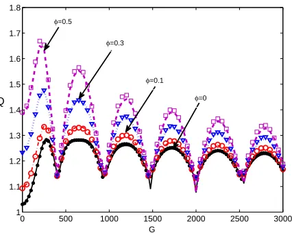
Further evidence for the possibility of enhancingQmax by variation of a dissipation parameter is presented in Fig. 4, for the response amplitude(s)Qas a function of the amplitude of the high frequency signal for four val-ues of phase shift φ, between the nonlinear dissipation and the periodic potential (φ = 0, φ = 0.1, φ = 0.3 and φ = 0.5). The numerically-computed Q from Eq. (29) using Eq. (25) (continuous and broken curves) and their corresponding analytically-calculated Q from Eq. (24) (solid shapes) are in agreement as clearly depicted by the close proximities of the location of the point mark-ers (analytic values) to their corresponding (of the same colour) continuous lines. Monotonic enhancement in the system’s response to modulation of the amplitude of the fast drive at resonance, similar to the effects produced by variation ofλis observed within a good choice of values of the driving signal parametersω, Ω andF. The value ofQmaxincreases with increasingφ, with the effect being more pronounced at low G. Since the damping is non-linear atφ= 0, the response curve atφ= 0 bears close resemblance to the behavior ofQat very weak values of the parameterλshown in Fig. 2. Forφ >0 presented in Fig. 4, increasing the phase differenceφproduces a signif-icant monotonic increase inQmax- the effect being more pronounced at lower values of the amplitude G of fast drive. Though multi-resonance is produced by varyingG in the presence of the slow signal, the system’s response at resonance can be enhanced or suppressed by adjust-ment of the phase φ. This shows that the dissipation parameters can indeed be used to control the system’s response at resonance: the dissipation parametersλand φare evidently able to control the resonance, as shown in Figs. 2 and 4.

Considering that the system’s potential and dissipation are both periodic ink, it implies that resonance can be induced by adjustment of the parameter k. The roles played by the ratio of the parameters of the fast signal in the occurrence of VR [57] can be performed/enhanced by k in a multiplicative fashion based on the ratio kG

Ω in Eq. (16), even when the parameters of the fast signal are fixed. Finally, for fixed values ofGand ω, and with variation ofk, the system can be driven into resonance as shown in Fig. 5 for three values ofG, namely, G = 250,G = 350 andG= 650. We have plotted in Fig. 5 the analytic response (filled circles) as obtained from Eq. (24) superimposed on the numerical response (Eq. (29)) obtained from Eq. (25) (curves) to demonstrate the good agreement. In addition, multiple resonance peaks occur at larger values ofGas observed in Fig. 5.

0.5 1 1.5

0.5 1 1.5

0 2 4 6 8 10

0.5 1 1.5

k Q

(b) G=350 (a) G=250

(c) G=650

FIG. 5: [Color Online] Dependence of the response amplitude Qon the control parameterkfor three amplitudes of fast forc-ing, G= 250, G= 350 andG= 650. The other parameters areγ0= 1.2,λ= 0.9,φ= 0.1,F = 0.1,ω= 0.65 and Ω = 13.

The continuous curves represent the numerically computedQ from Eq. (4) while the corresponding analytically calculated Qfrom Eq. (24) is shown as open circle (marker) points.

0

100

200

300

400

500 0

0.5 1

1.5 2

2.5 3 0

10 20

G

λ

Q

2 4 6 8 10 12 14 16 18 20

FIG. 6: [Color Online] 3-dimensional plot showing the depen-dence of the response amplitudeQon the fast signal ampli-tudeGand the dissipation parameter λfor a phase shift of φ = 0.85. Notice that small values ofGalso produce some low peaks in the regime marked in deep blue; while the largest peaks occur at higherGand lowerλ.

that can be obtained with weak dissipation (typically, λ < 2.0) and high amplitudes of the fast signal (typi-cally, G > 200). Elsewhere, however, weak resonances peaks can also appear and are indicated in blue.

B. Origin and mechanism of VR

We can now seek to understand the origin and mech-anism of VR by exploring the underlying dynamics and,

in particular, the bifurcation structure and attractors in Poincar´e section. Proceeding as before, we calculated the time-asymptotic motion of the system (25), visualiz-ing the trajectories as a series of points in (x, v) phase-space, where v = ˙x; and recording only one point per period of the external drive, i.e. a point is plotted when ωt=δ+n2πwhereδis the Poincar´e phase. Using a pa-rameter of the nonlinear dissipation, in this caseλ, as the bifurcation parameter we first examine the bifurcation structure. It is well known that in nonlinear systems, res-onance curves are closely linked to the underlying bifur-cation structure [27, 53, 60, 61]. In particular, Koz lowski et al. [61] and Roy-Layinde et al. [53] have shown that symmetry-breaking (sb) bifurcations occur between res-onances. Here, we report a new dynamical transition mechanism associated with resonance. Fig. 7 shows the forward bifurcation diagram (dotted red) obtained by in-creasing the value ofλfrom 0 to 4, the corresponding nu-merically computed response curveQ(dashed blue line), and the maximal Lyapunov exponent λmax (green line)

forG= 15. There is a clear and striking correlation be-tween theQplot andλmaxatλthr≈1.30 just before the Hopf bifurcation takes place for increasingλ. Preceding the Hopf bifurcation transition point,H (i.e. λ≈1.66), the system appears to be in a quiescent state wherein the strength of periodic nonlinear dissipation is incapable of exciting it into resonance. Within this regime, λmax

changes values fromλmax<0 (periodicity) toλmax≈0

(quasiperiodicity), at λthr ≈ 1.30 - a threshold dissipa-tion above which the system is excited into resonance, thereby signaling the onset of VR as shown, with the first resonant peak appearing atλ ≈1.85 and in the neigh-bourhood of the Hopf bifurcation; and thereafter, several resonance peaks emerges. Evidently, forλ > λthr ≈1.30,

Q first increases exponentially, and then experiences a sudden jump at the Hopf bifurcation point, H. Thus, the jump inQ signalling VR clearly originates from the Hopf bifurcation, thereby strongly suggesting that VR is linked to the bifurcation of the attractors.

To complete the picture, Fig. 8 illustrates the dynam-ical mechanism accompanying the bifurcation leading to VR, which shows the dynamics emerging from a peri-odic orbit for λ= 0 to enlarged quasiperiodic orbits as λincreases. We have plotted the orbits for five different values ofλto illustrate that further increase inλleads to a monotonic increase in the attractor size for other values ofλ >0. It is precisely the growth in attractor size of the attractor withλthat is responsible for the occurrence of VR, as characterized by the monotonic enhancement of peaks seen in Fig. 2 for increasing values ofλ.

V. CONCLUDING REMARKS

-0.2 -0.1 0 0.1 0.2 0.3

0 0.5 1 1.5 2 2.5

x, Q,

λmax

λ

λthr

H

FIG. 7: [Color Online] The bifurcation diagram (dotted red) of the displacement, x, the corresponding response curve Q (blue) and maximal Lyapunov exponent, λmax, (green) for

G= 15. The other parameters are fixed as follows: γ0= 1.2,

k= 1.0,φ= 0.85,V0= 1.0,F= 0.1,ω= 0.65, and Ω = 13.

-4 -2 0 2

-2 -1 0 1 2 3

v

x

λ = 0

λ = 1.35

λ = 1.4

λ = 1.5

λ = 2.0

FIG. 8: [Color Online] Transition from periodicity to quasiperiodicity accompanying the onset of VR with vari-ation of the dissipvari-ation parameter λ: periodic orbit for λ= 0 (red), monotonic quasiperiodic attractor enlargement forλ= 1.35(green),1.4(blue),1.5(magneta), and 2.0 (cyan). The other parameters are fixed at: G= 15,γ0= 1.2,k= 1.0,

φ= 0.85,V0= 1.0,F = 0.1,ω= 0.65, and Ω = 13.

a bi-harmonic signal. The contributions from both the parameters of the frictional inhomogeneity and from the fast signal in the resonant state were first identified based on the computed effective potential and the effective dis-sipation terms, from which we deduced that these could

be employed to induce and control resonances in a similar manner to the roles played by delay terms reported ear-lier [46, 62]. In contrast to the case of linearly damped systems, where the effective stiffness is the parameter of interest, we examined theoretically and confirmed nu-merically the contributions of the parameters of the high frequency signal to the system’s effective dissipation. We found that, within an appropriate parameter regime, VR can be significantly enhanced by varying the nonlinear dissipation parameters; and that it can be induced by a parameter that is commonly shared by the damping in-homogeneity and the system potential. Scanning the sys-tem in the (λ, G) two-parameter plane, we found that the regions of optimal resonance corresponds to low values of dissipation (λ < 2.0) and high values of the fast signal amplitude (G > 200); while elsewhere weak resonances occur. The underlying dynamics revealed that the origin of the nonlinear-dissipation-enhanced resonance could be linked to monotonic attractor enlargement arising from a Hopf bifurcation taking place near the onset of VR.

We remark that certain features of vibrational reso-nance have potential industrial applications including for output filtering, control and enhancement, signal detec-tion, extraction or separadetec-tion, noise reducdetec-tion, or high-lighting specific elements of a signal. More specifically, advanced technological applications exhibit better per-formance and efficiency when ratchet-like devices such as sensors, nonlinear mixers, filters, atomic scale imaging and amplifiers are operated in resonant modes – possibil-ities that can be fully explored in the near future. In controlling the motion of tiny particles in nanoscience or micro or macroscale oscillators [27], one could explore the optimal choice of dissipation parameters and of the fast input signals functioning as controllers, in order to dic-tate the direction of particle transport and maximise the flux. Finally, we comment that our model could imme-diately be realised experimentally in an electronic circuit including a Josephson junction with its external drives modeled as input voltage/current sources.

Acknowledgments

UEV is supported by the Royal Society of London, through their Newton International Fellowship Alumni scheme. The authors are indeed grateful to the review-ers for their constructive comments. The research was supported by the Engineering and Physical Sciences Re-search Council UK (grant No EP/M015831/1). No new data were created during this study.

[1] S. Elliott, M. Ghandchi Tehrani, and R. S. Langley, Phil. Trans. R. Soc. A373, 20140402 (2015).

[2] H. G. Enjieu Kadji, B. R. Nana Nbendjo, J. B. Chabi Orou, and P. K. Talla, Phys. Plasmas15, 032308 (2008).

[4] P. Silvestrini, J. Appl. Phys.68, 663 (1990).

[5] P. Silvestrini, Phys. Rev. B46, 5470 (1992).

[6] M. Siewe Siewe, H. Cao, and M. Sanjuan, Chaos, Solitons and Fractals39, 10921099 (2009).

[7] V. V. Semenov, A. B. Neiman, T. E. Vadivasova, and V. S. Anishchenko, Phys. Rev. E93, 052210 (2016).

[8] A. Eichler, J. Moser, J. Chaste, M. Zdrojek, I. Wilson-Rae, and A. Bachtold, Nat. Nanotech.6, 339 (2011).

[9] M. Imboden, O. Williams, and P. Mohanty, Appl. Phys. Lett.102, 103502 (2013).

[10] M. Imboden, O. A. Williams, and P. Mohanty, Nano Lett.

13, 4014 (2013).

[11] M. Imboden and P. Mohanty, Phys. Rep.534, 89 (2014).

[12] J. Atalaya, T. W. Kenny, M. L. Roukes, and M. I. Dyk-man, Phys. Rev. B94, 195440 (2016).

[13] J. R. Wright and J. E. Cooper,Introduction to Aircraft Aeroelasticity and Loads(John Wiley & Sons, New York, 2008).

[14] C. Surace, K. Worden, and G. R. Tomlinson, Proc. Inst. Mech. Eng., Part D: J. Automobile Eng.206, 3 (1992).

[15] U. Ingard and H. Ising, J. Acoust. Soc. Am.42, 60017 (1967).

[16] E. De Boer,Mechanics of the Cochlea: Modelling Efforts

(Springer,New York, NY, 1996).

[17] A. Roy, Z. Leghtas, A. D. Stone, M. Devoret, and M. Mir-rahimi, Phys. Rev. A91, 013810 (2015).

[18] D. Mogilevtsev, A. Mikhalychev, V. S. Shchesnovich, and N. Korolkova, Phys. Rev. A87, 063847 (2013).

[19] S. Saikia and M. C. Mahato, Physica A389, 4052 (2010).

[20] C. Mulhern, Phys. Rev. E88, 022906 (2013).

[21] L. Du and D. Mei, Phys. Rev. E85, 011148 (2012).

[22] S. Saikia and M. C. Mahato, Phys. Rev. E80, 062102 (2009).

[23] S. Saikia and M. C. Mahato, J. Phys.: Cond. Matt.21, 175409 (2009).

[24] S. Saikia, A. M. Jayannavar, and M. C. Mahato, Phys. Rev. E83, 061121 (2011).

[25] D. Kharkongor, W. L. Reenbohn, and M. C. Mahato, Phys. Rev. E94, 022148 (2016).

[26] S. Saikia, Physica A468, 219 (2017).

[27] S. Rajasekar and M. A. F. Sanjuan, Nonlinear Res-onances, Springer Series in Synergetics (Springer, Switzerland, 2016).

[28] M. I. Dykman, D. G. Luchinsky, R. Mannella, P. V. E. McClintock, N. D. Stein, and N. G. Stocks, Nuovo Ci-mento D17, 661 (1995).

[29] N. G. Stocks, N. D. Stein, S. M. Soskin, and P. V. E. McClintock, J. Phys. A: Math. Gen.25, L1119 (1992).

[30] L. Y. Chew, C. Ting, and C. H. Lai, Phys. Rev. E72, 036222 (2005).

[31] S. Nobukawa, H. Nishimura, and T. Yamanishi, Scientific Reports p. 1331 (2017).

[32] A. S. Pikovsky and J. Kurths, Phys. Rev. Lett.78, 775 (1997).

[33] O. V. Ushakov, H. J. W¨unsche, F. Henneberger, I. A. Khovanov, L. Schimansky-Geier, and M. A. Zaks, Phys. Rev. Lett.95, 123903 (2005).

[34] J. Casado-Pascual, J. G´omez-Ord´onez, and M. Morillo, Chaos15, 26115 (2005).

[35] S. Rajamani, S. Rajasekar, and M. A. F. Sanjun, Comm. Nonlin. Sc. Num. Sim.19, 4003 (2014).

[36] P. S. Landa and P. V. E. McClintock, J. Phys. A: Math. Gen.33, L433 (2000).

[37] R. Jothimurugan, K. Thamilmaran, S. Rajasekar, and

M. A. F. Sanju´an, Nonlin. Dyn.83, 1803 (2016).

[38] M. Gitterman, J. Phys. A: Math. Gen.34, L355 (2001).

[39] I. Blekhman and P. Landa, Intern. J. Non-Lin. Mech.39, 421 (2004).

[40] S. Jeyakumari, V. Chinnathambi, S. Rajasekar, and M. A. F. Sanjuan, Chaos19, 043128 (2009).

[41] Y. Qin, J. Wang, C. Men, B. Deng, and X. Wei, Chaos

21, 023133 (2011).

[42] S. Rajasekar, J. Used, A. Wagemakers, and M. Sanjuan, Commun. Nonlin. Sci. Num. Sim.17, 3435 (2012).

[43] V. N. Chizhevsky, Phys. Rev. E89, 062914 (2014).

[44] K. Abirami, S. Rajasekar, and M. Sanjuan, Commun. Nonlin. Sci. Numer. Sim.47, 370 (2017).

[45] S. Guruparan, V. Ravichandran, V. Chinnathambi, and S. Rajasekar, Ukrainian J. Phys.62, 51 (2017).

[46] J. H. Yang and X. B. Liu, Chaos20, 033124 (2010).

[47] J. H. Yang and X. B. Liu, J. Phys. A: Math. Theor.43, 122001 (2010).

[48] C. Jeevarathinam, S. Rajasekar, and M. A. F. Sanjuan, Phys. Rev. E83, 066205 (2011).

[49] A. Daza, A. Wagemakers, S. Rajasekar, and M. Sanjuan, Commun. Nonlin. Sci. Num. Sim.18, 411 (2013).

[50] J. Yang and H. Zhu, Chaos22, 013112 (2012).

[51] T. L. M. D. Mbong, M. S. Siewe, and C. Tchawoua, Mech. Res. Commun.78, Part A, 13 (2016).

[52] T. L. M. D. Mbong, M. S. Siewe, and C. Tchawoua, Com-mun. Nonlin. Sci. Numer. Sim.22, 228 (2015).

[53] T. O. Roy-Layinde, J. A. Laoye, O. O. Popoola, and U. E. Vincent, Chaos26, 093117 (2016).

[54] B. Deng, J. Wang, X. Wei, H. Yu, and H. Li, Phys. Rev. E89, 062916 (2014).

[55] M. Borromeo and F. Marchesoni, Phys. Rev. E 73, 016142 (2006).

[56] B. S. Dandogbessi, O. Akin-Ojo, and A. Kenfack, Phys. Scrip.90, 055206 (2015).

[57] S. Rajasekar, K. Abirami, and M. A. F. Sanjuan, Chaos

21, 033106 (2011).

[58] M. Imboden and P. Mohanty, Physics Reports 534, 89 (2014).

[59] A. Cleland, New J. Phys.7, 787 (2005).

[60] U. Parlitz and W. Lauterborn, Phys. Lett. A107A, 351 (1985).

[61] J. Koz lowski, U. Parlitz, and W. Lauterborn, Phys. Rev. E51, 1861 (1995).

[62] C. Jeevarathinam, S. Rajasekar, and M. Sanjuan, Chaos