Decoding solar wind-magnetosphere coupling
M. J. Beharrell1and F. Honary1
1Physics Department, University of Lancaster, Lancaster, UK
Abstract
We employ a new NARMAX (Nonlinear Auto-Regressive Moving Average with eXogenous inputs) code to disentangle the time-varying relationship between the solar wind andSYM-H. The NARMAX method has previously been used to formulate aDstmodel, using a preselected solar wind coupling function. In this work, which uses the higher-resolutionSYM-Hin place ofDst, we are able to reveal the individual components of different solar wind-magnetosphere interaction processes as they contribute to the geomagnetic disturbance. This is achieved with a graphics processing unit (GPU)-based NARMAX code that is around 10 orders of magnitude faster than previous efforts from 2005, before general-purpose programming on GPUs was possible. The algorithm includes a composite cost function, to minimize overfitting, and iterative reorthogonalization, which reduces computational errors in the most critical calculations by a factor of∼106. The results show that negative deviations inSYM-Hfollowing a southwardinterplanetary magnetic field (IMF) are first a measure of the increased magnetic flux in the geomagnetic tail, observed with a delay of 20–30 min from the time the solar wind hits the bow shock. Terms with longer delays are found which represent the dipolarization of the magnetotail, the injections of particles into the ring current, and their subsequent loss by flowout through the dayside magnetopause. Our results indicate that the contribution of magnetopause currents to the storm time indices increase with solar wind electric field,E=v×B. This is in agreement with previous studies that have shown that the magnetopause is closer to the Earth when the IMF is in the tangential direction.
1. Introduction
The interaction of the solar wind and Earth’s magnetosphere, beginning when an element of the solar wind impacts the dayside magnetopause, is a process that lasts several hours, evolving as the solar wind progresses around the magnetosphere. On the nightside, particles are injected into the ring current and accelerated as the magnetic field dipolarizes. The populations of these particles subsequently decay in a number of ways, including charge exchange with the upper atmosphere (particle precipitation) and flowout from the dusk and dayside magnetopause. Each stage of the interaction has a unique effect onDst, a measure of the geomagnetic disturbance field on Earth.
There can be no doubt that the populations of energetic particles in the inner magnetosphere are enhanced during geomagnetic storms nor that these particles contribute to negative excursions of theDstindex. To a first approximation the magnetic effect of the particles can be calculated with the Dessler-Parker-Sckopke (D-P-S) relation [Dessler and Parker, 1959;Sckopke, 1966], which is written in modern terms as
𝜇⋅b(0) =2UK, (1)
whereb(0)is the (vector) average disturbance field over the surface of the Earth,𝜇is the dipole moment, and UKis the total kinetic energy of the plasma in the magnetosphere. The particles are primarily injected and
accelerated on the nightside, as the tail magnetic field reconnects and relaxes to a more dipolar configuration. Traditionally, a magnetic storm is considered to be a rapid succession of these dipolarization-injection events, which are called substorms. However, the findings ofIyemori and Rao[1996] appear to contradict this picture. They report that theDstindex decays (becomes less negative) after substorm onset.Siscoe and Petschek[1997] provides an explanation: during substorm onset the magnetic energy contained in the stretched magnetotail is transferred to charged particles in the ring current, but the stretched magnetotail itself has aDst contri-bution, which is reduced during dipolarization. Further evidence of this is provided byLopez et al.[2015], who report that during the magnetic storm of 31 March 2001,SYM-Hwas observed to decrease by more than 200 nT without any ring current enhancement but with growth of the magnetotail. During the storm,
RESEARCH ARTICLE
10.1002/2016SW001467
Key Points:
• Empirical model of
SW-magnetosphere coupling gives insight into the various mechanisms and provides formulas to quantify their effects
• New GPU-based NARMAX code is used: 1 million times more precise and 10 billion times faster than previous efforts
• Very small changes in SYM-H that occur on short timescales can be accurately reproduced by the model using just solar wind data
Correspondence to:
M. J. Beharrell,
Citation:
Beharrell, M. J. and F. Honary (2016), Decoding solar wind-magnetosphere coupling,Space Weather,14, 724–741, doi:10.1002/2016SW001467.
Received 11 JUL 2016 Accepted 14 SEP 2016
Accepted article online 19 SEP 2016 Published online 6 OCT 2016
©2016. The Authors.
a large injection also coincided with a positive change (loss) inSYM-H. Earlier,Siscoe[1970] had extended the D-P-S relation to include the magnetic field energyUb,
𝜇⋅b(0) =2UK+Ub. (2)
The influence of the ring current kinetic energy on the disturbance field is twice that of the magnetic energy. This means that when the magnetotail dipolarizes, and magnetic energy from the tail is transferred to the ring current, there will be a decay in theDstindex if more than half of the magnetotail energy is lost elsewhere. On the other hand, if more than 50% of the energy stored in the tail is transferred to the ring current, there will be an increase in−Dst. A substantial part of the magnetic energy transferred from the solar wind in the merging, convecting, and separating of the geomagnetic field and the interplanetary magnetic field (IMF) is lost down-stream as a plasmoid during the substorm expansion process and as Joule heating in the ionosphere.Wang et al.[2014] estimate that 13% of the solar wind kinetic energy is transferred to the magnetosphere. The input energy is roughly equally divided between the auroral ionosphere, the ring current, and the plasmoid [Ieda et al., 1998;Kamide and Baumjohann, 1993]. The portion of energy that remains in the enhanced ring current persists and builds up over the course of a geomagnetic storm.
Typically, the first change seen inDstat the beginning of a storm is a positive swing, due to an increase in the dayside magnetopause current from an enhanced solar wind dynamic pressure. The injection of energetic particles into the ring current, resulting in prolonged negativeDstvalues, occurs primarily on the nightside. It takes time, of the order of an hour, for newly merged IMF and geomagnetic field lines to convect to the nightside of the planet and diffuse through the magnetotail, at which point the open geomagnetic field reconnects (closes) and undergoes dipolarization. Many formulas are available that describe the negative excursions ofDstin terms of the solar wind parameters; some of these are listed in section 5. These “coupling functions” are often (incorrectly) assumed to directly represent the rate of particle injection into the ring current, but it is no coincidence that the functions appear to describe the rate of magnetic field merging on the dayside. Following the explanation ofSiscoe and Petschek[1997], the merging of magnetic flux on the dayside results in a negative swing inDstfirst due to the deformation of the magnetotail and the enhanced cross-tail current. Around an hour later, when this merged flux reconnects on the nightside, the injection of particles into the ring current offsets the loss ofDstfrom the restored geomagnetic field. At this point the neg-ativeDstcontribution is transferred from the magnetic field to an enhanced ring current. Recently,Vasyli¯unas [2006] points out that the deformation of the geomagnetic tail can be represented by the amount of open (merged) magnetic flux, which is largely piled up in the magnetotail. If during tail reconnection the gain in −Dstfrom the ring current exactly cancels the loss from the reduced magnetotail contribution, then the cou-pling functions, which describe the enhancement of−Dstover the course of a storm, will be identical to the rate of dayside magnetic field merging. However, there is no reason to believe that exactly half of the mag-netotail energy is transferred to the ring current, so that its contribution toDstexactly replaces that of the deformed magnetotail.
The low time resolution ofDsthas no doubt hampered past efforts to examine the coupling processes in detail. By using the higher-resolution but otherwise equivalentSYM-H[Wanliss and Showalter, 2006], we aim to dis-cover formulas describing changes in the disturbance magnetic field for each of the mechanisms described in this section. These include the magnetopause currents, magnetotail currents, magnetotail reconnection and particle injection, flowout through the magnetopause, and atmospheric charge exchange losses. To this end, we employ a new NARMAX code (Nonlinear Auto-Regressive Moving Average with eXogenous inputs). NARMAX has previously been used to formulate a 1 h resolutionDstmodel, using a preselected coupling function [Boynton et al., 2011]. The choice of coupling function (described inBoynton et al.[2011]) is made using the OLS-ERR (Ordinary Least Squares-Error Reduction Ratio) algorithm. OLS-ERR is commonly used to select NARMAX model terms; here it was used to choose from approximately 3600 candidate coupling functions. While theBoynton et al.[2011] model provides a good approximation toDst, the use of a sin-gle coupling function at 1 h time resolution suggests that the function represents a mixture of the various coupling processes.
2. Theory
higher-resolutionSYM-Hindex.SYM-His equivalent toDstbut sampled at 1 min resolution [Wanliss and Showalter, 2006]. The Burton-Mcpherron-Russell continuity equations forDst[Burton et al., 1975] can therefore be written in terms ofSYM-H.
SYM-H∗=SYM-H−b√p+c, (3)
dSYM-H∗
dt =Q−
SYM-H∗
𝜏 , (4)
where SYM-H∗ is a pressure-correctedSYM-H, i.e., with the Chapman-Ferraro (magnetopause) currents removed. To a first approximationbis usually assumed to be a constant, its value determined by the geometry of the dayside magnetopause. The parametercis also assumed to be a constant.Qis a source term represent-ing the injection of charged particles into the rrepresent-ing current, andSYM-H∗∕𝜏represents an idealized exponential decay of the ring current. More recently, it has become apparent that other important terms exist, and these should be added to theSYM-Hcontinuity equation. Flowout, where particles entering the magnetosphere on quasi-trapped orbits drift out of the dayside magnetopause, is especially significant during storms [Kozyra and Liemohn, 2003]. Changes observed inDstthat are associated with the well-known solar wind coupling functions are commonly but incorrectly thought to be a direct measurement ofQ, the injection of particles into the ring current.Vasyli¯unas[2006] points out that the effects described by the coupling function are first due to the increasing magnetic flux in the magnetotail. Therefore,DstandSYM-Hmust depend on the flux of open geomagnetic field lines, the majority of which are piled up in the magnetotail. The total rate of change of open magnetic flux can be written as the opening rate of flux on the dayside minus the closing rate on the nightside.
dSYM-H∗
dt =Q+F−
SYM-H∗
𝜏 −a
(d Φd dt −
dΦn dt
)
, (5)
where the coefficientaprovides the conversion from magnetic flux in the tail toSYM-Hon the ground;dΦd
dt is
the rate of flux opening on the dayside and piling up in the tail, anddΦn
dt is the rate of flux closing in nightside
reconnection.Fis the rate of flowout from the dayside magnetopause. Note that the sign ofQis negative, as particles entering the magnetosphere increase−SYM-H, whereasFis positive.
Equation (5) is converted to use discrete time steps,Δt, andSYM-His substituted forSYM-H∗using equation (3),
SYM-H−B−1= (
1−Δt 𝜏
) (
SYM-H−1−B−1) (6a)
+bΔ√p (6b)
−aΔΦd (6c)
+(aΔΦn+QΔt) (6d)
+FΔt, (6e)
whereB(=b√p)is the best known approximation of the pressure correction. It does not need to be highly accurate because the same value (B−1) is deducted from bothSYM-HandSYM-H−1, andΔt∕𝜏is small. This
cor-rection is applied to theSYM-Hdata before analysis begins. An initial run of the NARMAX code then provides a better value ofb√pfrom the term (6b). The analysis is rerun using the improved pressure correction asB. In our analysisbis not restricted to a constant. The NARMAX method searches for functions based on the solar wind parameters to represent each of the terms (6a) to (6e).
ΔΦnis the amount of magnetic flux closed by magnetic reconnection on the nightside during the interval Δt. In equation (6) it is placed withQ, the injection of particles into the ring current, because both processes occur simultaneously and are difficult or impossible to separate empirically with analysis of solar wind and SYM-Hdata.
into the tail. The differences in the lag times are exploited by the NARMAX model selection technique to decode the time series ofSYM-Hand solar wind data. In this paper a fast NARMAX code is used to find functions of solar wind parameters that best represent each of the five terms in equation (6).
3. Data
The solar wind data we use, spanning 1 January 1995 to 1 June 2013, are taken directly from the OMNI2 data set [King and Papitashvili, 2006]. Although solar wind data are available from as early as the 1960s, in an attempt to avoid possible bias from the varying sources we use only data from after 1995, which is provided by the newer ACE and WIND spacecraft. This has the additional benefit of reducing the size of the data set and speeding up the calculations. Data between 17 March 2000 and 9 May 2000 are excluded. This is a period with few data gaps and is therefore ideal for validating the model. The OMNI2 magnetic field and plasma data have been time shifted to compensate for the location of the spacecraft, which are approximately 1 h upstream of the Earth. The solar wind data are combined withSYM-Hand integrated to 5 min samples.
It is advantageous to run the NARMAX algorithm on multiple subsets of the data. Comparing the results obtained for each subset shows the level of consistency of the model results and reveals any overfitting. Splitting the data set requires some care. If the data are split at a particular epoch, there may be a bias in the results if, for example, the earlier data set is recorded during a different part of the solar cycle or during a different season to the latter part of the data set. Separating the data set on a sample-by-sample basis is also problematic, as neighboring samples will be far from independent, and the two data sets will be nearly identical. Instead, the data are grouped into week-long segments, each containing 2016 samples (5 min resolution). The week-long segments are randomly distributed between two data sets: a training set and a testing set. This method gives two independent and unbiased data sets, which are made as close in size as possible. The NARMAX algorithm is run on one of the two halves of data, while the other half is used to check the quality of the result as each term is selected. The model result is labeled “1A.” Next, the two subsets of data are switched around, with the training set becoming the testing set, and vice versa, and the result is labeled “1B.” The results 1A and 1B are based on separate data sets; i.e., no samples are used by the NARMAX code for both models 1A and 1B. The data randomization procedure is repeated, with the week-long segments again being distributed randomly between two new subsets of data. This time the results are labeled 2A and 2B. While 2A and 2B are produced using separate data sets, there is some overlap between the data used for 1A and 2B, for example. The procedure is repeated five times, giving a total of 10 NARMAX model results for comparison.
4. The NARMAX Technique
The goal of the NARMAX method is to produce a model for a response variable,y(t), in the form
y(t) =
M
∑
k=1
pk(t)𝜃k+𝜉(t), (7)
wheretis the sample number (1, 2,…,N),pk(t)is thekth predictor out of a total ofM, and𝜃kis the coefficient of that predictor. The term𝜉(t)is the uncorrelated model residual, i.e., the part ofy(t)that cannot be repre-sented by any of the predictor terms. In our case the outputy(t) = SYM-H∗(t)and each of theMpredictor terms is a different product of the various solar wind parameters andSYM-H∗values, with a range of lag times.
For example, one of the parameters could be density×pressure at a lag of 10 min, and another could be SYM-H∗2× pressure2 with a 15 min lag. The NARMAX method seeks to identify the mmost important
predictors (typically between 5 and 20) and provide their coefficients. The number of candidate predictor terms,M, can clearly be very large when there are more than a few lags and solar wind parameters, so the candidates are limited to a particular degree of nonlinearity (the sum of all of the powers in the product).
is not present in any of the other selected terms. The NARMAX method achieves this by orthogonalizing the candidate predictor vectors,pk, with respect to the previously selected and orthogonalized predictor vectors, w1,w2,…,wk−1.
In vectorized form, equation (7) can be written as
y=P𝚯+𝚵, (8)
wherePis a matrix formed by the candidate predictor vectors, withMcolumns andNrows.𝚯is the vector of coefficients.Pcan be decomposed into a product of an orthogonal matrixWand an upper triangle matrixA.
P=WA, (9)
where
W= ⎡ ⎢ ⎢ ⎢ ⎢ ⎣
w1(1) w2(1) w3(1) … wM(1)
w1(2) w2(2) w3(2) … wM(2)
⋮ ⋮ ⋮ ⋱ ⋮
w1(N) w2(N) w3(N) … wM(N)
⎤ ⎥ ⎥ ⎥ ⎥ ⎦
. (10)
Every column ofWis orthogonal to every other column, and each is a vector,wk, representing a time series of thekth variable. It is not practical or necessary to compute the full orthogonal matrixW; instead, only the firstmcolumns are filled with thewkvectors that correspond to the bestmpredictors. These predictors are usually selected by the NARMAX algorithm according to the value of the error reduction ratio,[ERR]k,
[ERR]k= (
wT ky
)2
wT kwk yTy
. (11)
At thekth selection, the remaining candidates are each orthogonalized relative to the previously selected basis vectors,w1,w2,…,wk−1. The candidate with the largest[ERR]kis selected to be thekth parameter. The selection process can be terminated when a desired tolerance,𝜌, is reached
1−
m
∑
k=1
[ERR]k< 𝜌. (12)
For a more complete description of the NARMAX model selection technique see, e.g.,Billings[2013]. To improve the accuracy of the orthogonalization calculations in the NARMAX algorithm, iterative reorthogo-nalization [Hoffmann, 1989] is implemented, to ensure that the selected orthogonal vectors,wk, are precisely
orthogonal. Testing showed this to produce an improvement in orthogonality of a factor of around 105to 106,
enabling the code to select the best terms even where there is a high level of ill conditioning.
In an attempt to minimize overfitting, a composite cost function is employed following the method ofHong and Harris[2001]. Its purpose is to penalize covariance between the selected parameters and minimize model prediction errors. The cost function,𝛼, is a small positive scalar parameter that balances the model’s approximation capability against its tendency to over fit the data. Instead of maximizing ERR, we maximize
ERR−𝛼 (
N
wT kwk yTy
)
. (13)
𝛼that would lead topkbeing the chosen regressor. The𝛼kthat is closest to the current𝛼is used for the next iteration of the model. For our data set it typically requires 15 to 20 values of𝛼to cover the whole of𝛼-space, from 0 to the value of𝛼for which no terms are selected for the model.
The NARMAX code was implemented in OpenCL and run on a single AMD Radeon R9 290X graphics card. OpenCL allows the algorithm to be programmed at a low level, with efficient use of the 2816 stream pro-cessors, registers, caches, and 4 GB of onboard RAM. The code scales well, with each model run in this paper taking 1 to 14 h. Extrapolating the CPU times given byBillings and Wei[2005, Table 1] suggests a CPU time of the order of tens of millions of years to complete a single model run of the current work. Of course, some of this speedup, perhaps a factor of 1000×, is due to today’s availability of fast and highly parallel graphics processing units (GPUs) and the overall advances in computer performance over the last decade.
5. Parameter Choices for Model Selection
The measurement parameters utilized in the NARMAX model are carefully chosen to ensure that the predictor variables are capable of reproducing equation (6). In order to accurately and precisely determine the unknown functions in the equation, a large range of exponents with small intervals are required in the candidate terms. The chosen measurement parameters are
|SYM-H∗|1∕2Δ√p, p1∕3,p1∕12,p−1∕2n3∕2,n1∕3,n1∕12E1∕2,E1∕3,E1∕12sin𝜃
2, and sin
4𝜃
2, (14)
whereE(=vBT), used throughout this paper, is the solar wind electric field in units of mV m−1;pis the dynamic
solar wind pressure in nanopascals;nis the solar wind proton number density in cm−3; and𝜃is the IMF
clock angle.
Lags of the solar wind parameters, ranging from 5 min to 4 h, are added to the data set. To reduce computation time, the longer lags are spaced at intervals. Lags of 5 to 60 min are spaced at 5 min intervals (i.e., without gaps), 60 to 120 min lags are spaced at 10 min intervals, and lags greater than 2 h are spaced at 15 min intervals.
Products of these parameters form the predictors in the NARMAX model, which are constructed up to a non-linearity degree of 8. In other words, each candidate term in the NARMAX model comprises up to eight of the measurement parameters multiplied together, with the same parameter able to appear more than once in each term. In forming the candidate predictor terms only solar wind parameters with the same lag are included in each term. A single 5 min lag of the|SYM-H∗|1∕2parameter is included. This is combined in the
candidate terms with solar wind parameters of any lag. For example, one of the candidate predictors will be [|SYM-H∗|1∕2
(t−5m)]3⋅[n1∕3(t−45m)]1⋅[E1∕2(t−45m)]2. In total there are 4,770,710 candidate predictors,
including a constant term.
The NARMAX algorithm does not work with missing data, so any samples that contain missing data (in any of the lags from 0 min to 4 h) are excluded. The remaining data comprises 1,175,732 samples.
Some examples of previously suggested coupling functions that are included in the candidate terms, with each of the aforementioned lags, are the following:
1.Kan and Lee[1979]:vBTsin2𝜃 2 =E
1∕2⋅E1∕2⋅sin𝜃 2⋅sin
𝜃
2(nonlinearity degree 4)
2.Wygant et al.[1983]:vBTsin4𝜃2
3.Scurry and Russell[1991]:vBTsin4𝜃2p1∕2
4.Temerin and Li[2006]:n1∕2v2B
Tsin6𝜃2
These and many other variations of the coupling functions could be selected by NARMAX to be included in the model’s approximation of equation (6). Similarly, the algorithm is able to choose different functions of the solar wind parameters for the other terms in equation (6). For example, if the coefficientbis better approximated by one of these functions, instead of a constant, that function will be selected. If the true Chapman-Ferraro term is proportional toΔ√3p, instead ofΔ√p, the model is able to selectΔ√p⋅p−1∕2⋅p1∕3as a close approximation.
6. Results
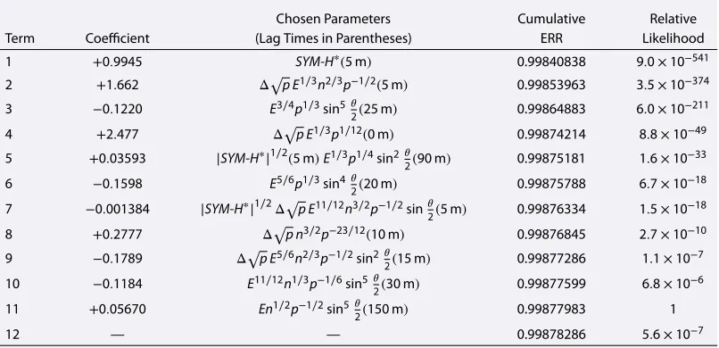
Table 1.Results From Run 1A of the NARMAX Codea
Chosen Parameters Cumulative Relative
Term Coefficient (Lag Times in Parentheses) ERR Likelihood
1 +0.9945 SYM-H∗(5m) 0.99840838 9.0×10−541
2 +1.662 Δ√p E1∕3n2∕3p−1∕2(5m) 0.99853963 3.5×10−374 3 −0.1220 E3∕4p1∕3sin5𝜃
2(25m) 0.99864883 6.0×10− 211
4 +2.477 Δ√p E1∕3p1∕12(0m) 0.99874214 8.8×10−49
5 +0.03593 |SYM-H∗|1∕2
(5m)E1∕3p1∕4sin2𝜃
2(90m) 0.99875181 1.6×10 −33
6 −0.1598 E5∕6p1∕3sin4𝜃
2(20m) 0.99875788 6.7×10
−18
7 −0.001384 |SYM-H∗|1∕2Δ√p E11∕12n3∕2p−1∕2sin𝜃
2(5m) 0.99876334 1.5×10− 18
8 +0.2777 Δ√p n3∕2p−23∕12(10m) 0.99876845 2.7×10⁻¹⁰ 9 −0.1789 Δ√p E5∕6n2∕3p−1∕2sin2𝜃
2(15m) 0.99877286 1.1×10 −7
10 −0.1184 E11∕12n1∕3p−1∕6sin5𝜃
2(30m) 0.99877599 6.8×10− 6
11 +0.05670 En1∕2p−1∕2sin5𝜃
2(150m) 0.99877983 1
12 — — 0.99878286 5.6×10⁻⁷
aThe 11-term model has the highest likelihood, calculated by comparing the model results at each stage against a separate data set, using the Bayesian Information Criterion.
SYM-H∗(t) =0.9945SYM-H∗(t−5m), which describes an exponential decay ofSYM-H∗, with a time constant
of 15.1 h. To a first approximation this model describes the decay of the ring current in the absence of energy input from the solar wind.
The standard method of measuring the significance of a term in NARMAX is with the error reduction ratio (ERR). The higher the ERR value of a term, the closer it will allow the model to fit the data. The sum of ERR values approaches 1 as the model becomes more complicated and fits the data more precisely. However, at some point the model will likely become overfitted as new model terms are fitting to measurement errors instead of real physical processes. To address this, the relative likelihood of each term is calculated from the Bayesian Information Criterion (BIC), using the testing half of the data set, which is assumed to be independent of the training data used by the NARMAX code. The cumulative ERR and relative likelihood at each step of the model selection are given in Table 1. They indicate that the most likely model has 11 terms, with subsequent terms leading to overfitting.
The composite cost function ofHong and Harris[2001] was employed, and the model was computed with a number of different values of the cost function,𝛼. In all but one of our model runs, the model with𝛼=0 provides the best fit to the testing data set, according the BIC. The single run that was improved with a nonzero
Figure 1.BIC-derived relative likelihood of each NARMAX result, using data set 2A, as a function of the cost function𝛼.
cost function was run 2A. The rela-tive likelihood of the models of run 2A, as a function of𝛼, are shown in Figure 1. Composite cost functions are an effective means of reducing overfit-ting, and the reason they are not espe-cially helpful here is that the data sets are large (∼600,000 samples, com-pared to 100 in the example given by Hong and Harris[2001]).
[image:7.612.191.404.534.718.2]Most of the terms given in Table 1 begin to look very familiar, as almost identical terms are seen in each of the 10 NARMAX runs. The terms are described briefly below and in more detail in the next section.
The second most significant term chosen by the NARMAX algorithm has a positive coefficient, short lag time, and containsΔ√p. These properties, which are also shared with terms 4 and 8, are associated with the Chapman-Ferraro (magnetopause) currents, corresponding to equation (6b).
Terms 3, 6, and 10 resemble the coupling functions listed in the previous section. They are functions ofEand sin𝜃
2, with negative coefficients, and lag times that are consistent with the time it takes solar wind to transverse
the magnetosphere and pile up in the magnetotail. The negative coefficients mean that an enhancement in the IMF-magnetosphere dayside merging rate will result in larger negativeSYM-Hvalues 20 to 30 min later. These terms represent equation (6c).
The fifth term appears to be essentially the geometric mean of the first term (a decay term) and the coupling function terms. The lag time associated with the coupling component is 90 min, which is approximately the time it takes merged magnetic field lines to transverse the magnetosphere, diffuse through the magnetotail, and begin to reconnect. We associate this term with the loss ofSYM-Has the open magnetic field in the mag-netotail reconnects, injecting particles into the ring current. In this process energy is lost primarily by Joule heating in the ionosphere and in the plasmoid escaping downwind. This term represents equation (6d).
We are unable to attribute term 7 to any physical process. The decrease in the model’s relative likelihood with the inclusion of this term indicates that it is anomalous. In other words, when this term is included the model becomes a worse fit for the testing data set.
Term 9 has a lag of 15 min. It represents a combination of two physical processes that overlap slightly in lag times: the Chapman-Ferraro current terms, with typical lags of 0 to 10 min, and the coupling function terms (3, 6, and 10), which typically have 20 to 30 min lag times. The overlap can be explained by the natural variation of lag times during different solar wind conditions. Lags will be shortened when the solar wind is fast. Errors in time shifting of OMNI solar wind data from the L1 Lagrange point to Earth orbit may also increase the spread of lag times calculated for each process.
Term 11 has the longest lag of all of the NARMAX selected terms, at 150 min. It is similar in form to the dayside magnetic field merging (coupling) terms, but it has a positive coefficient indicative of a loss term. The rate of merging of the IMF and the geomagnetic field is expected to be proportional to the subsequent, delayed, injection of particles into the ring current. These particles drift from the nightside injection region to the day-side in approximately 1 h. The lag of this term is 60 min longer than that of term 5, which is associated with the injection of particles into the ring current. It is likely that this term represents a first approximation of the flowout of ring current particles through the dayside magnetopause. This is equation (6e).
In the next sections we discuss each of the terms in more detail and offer explanations for their forms.
7. Discussion
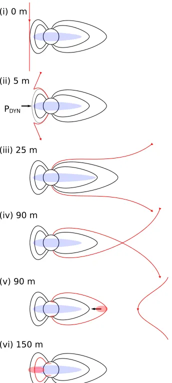
Tables 2–5 list all of the identified terms in each of the model runs. The consistency of the functions found using different sets of data provides a level of confidence in the results. Note that the coefficients alone do not represent the significance of each model term, because the functions vary. Figure 2 provides a schematic of the coupling mechanisms associated with these terms and shows their respective lag times, relative to the moment an element of solar wind reaches the bow shock.
7.1. Charge Exchange Losses
In every model run the first predictor selected by the NARMAX algorithm is simply the 5 min lag ofSYM-H∗.
The coefficient of this term is slightly less than 1, and therefore it represents an exponential decay inSYM-H. It is identified as equation (6a). The mean exponential time scale,𝜏, given by the model runs is 17.6 h, with a standard deviation of 2.2 h. This loss term is primarily associated with charge exchange between ring current particles and the upper atmosphere, because, unlike other identified loss mechanisms described later, the rate of charge exchange depends on the overall number of particles in the ring current.
7.2. Currents Induced by Solar Wind Pressure
Table 2.NARMAX Model Terms Associated With Solar Wind Dynamic Pressurea
Run 0 Min Lag 5 Min Lag 10 Min Lag
1A +2.477E1∕3p1∕12Δ√p +1.662E1∕3n2∕3p−1∕2Δ√p +2.777×10⁻¹n3∕2p−23∕12Δ√p 1B +2.115E1∕2Δ√p +1.472E1∕2n2∕3p−2∕3Δ√p +1.498×10⁻¹n11∕6p−2Δ√p 2A +2.080E5∕12p1∕12Δ√p +1.546E1∕2n2∕3p−2∕3Δ√p +2.571×10⁻¹n3∕2p−11∕6Δ√p
2B +2.803E1∕3n−1∕6p1∕4Δ√p +1.634E1∕3n2∕3p−1∕2Δ√p +2.812×10⁻¹n3∕2p−23∕12Δ√p 3A +2.474E5∕12Δ√p +1.665E5∕12n2∕3p−2∕3Δ√p +3.228×10⁻¹n3∕2p−11∕6Δ√p 3B +2.069E5∕12p1∕12Δ√p +1.426E1∕3n2∕3p−1∕2Δ√p +2.577×10⁻¹n3∕2p−23∕12Δ√p 4A +2.791E1∕3n−1∕6p1∕4Δ√p +2.025E1∕3n1∕2p−5∕12Δ√p +1.690×10⁻¹n11∕6p−2Δ√p 4B +2.307E5∕12Δ√p +1.645E5∕12n2∕3p−2∕3Δ√p +3.114×10⁻¹n3∕2p−23∕12Δ√p 5A +2.715E1∕3n−1∕6p1∕4Δ√p +1.601E5∕12n2∕3p−2∕3Δ√p +3.142×10⁻¹n3∕2p−11∕6Δ√p 5B +2.344E5∕12Δ√p +1.502E1∕2n2∕3p−2∕3Δ√p +2.738×10⁻¹n3∕2p−23∕12Δ√p
[image:9.612.174.567.314.494.2]aThese terms represent equation (6b).
Table 3.Traditionally Referred to as Coupling Functions, These Terms in the NARMAX Model Runs Are Associated With the Merging of the IMF and Geomagnetic Field (Equation (6c))a
Run 20 Min Lag 25 Min Lag Lags Given in Parentheses
1A −1.598×10⁻¹E5∕6p1∕3sin4𝜃
2 −1.220×10−
1E3∕4p1∕3sin5𝜃
2 −1.184×10−
1E11∕12n1∕3p−1∕6sin5𝜃 2(30m) 1B −2.130×10⁻¹E3∕4p1∕3sin4𝜃
2 −1.564×10
−1E11∕12n1∕6sin5𝜃
2 −5.954×10
−2En1∕3n1∕3p−1∕12sin5𝜃 2(35m) 2A −2.429×10⁻¹E3∕4p5∕12sin5𝜃
2 −1.423×10−
1En1∕3p−1∕6sin5𝜃 2(30m) 2B −1.694×10⁻¹E11∕12p1∕4sin5𝜃
2 −2.476×10
−1E3∕4p1∕3sin4𝜃 2 3A −1.763×10⁻¹E5∕6p1∕3sin5𝜃
2 −1.272×10
−1E5∕6p1∕4sin5𝜃
2 −9.254×10
−2En1∕3p−1∕6sin5𝜃 2(30m) 3B −2.451×10⁻¹E3∕4p5∕12sin5𝜃
2 −1.787×10−
1E11∕12n1∕6sin4𝜃 2(30m) 4A −2.511×10⁻¹E3∕4p5∕12sin5𝜃
2 −1.795×10
−1E11∕12n1∕6sin4𝜃 2(30m) 4B −1.866×10⁻¹E5∕6p1∕3sin5𝜃
2 −1.107×10−
1E3∕4p1∕3sin4𝜃
2 −1.326×10−
1E11∕12n1∕6sin4𝜃 2(30m) 5A −2.372×10⁻¹E3∕4p5∕12sin5𝜃
2 −1.824×10
−1E11∕12n1∕6sin4𝜃 2(30m) 5B −1.782×10⁻¹E5∕6p1∕3sin5𝜃
2 −2.273×10
−1E3∕4p1∕3sin4𝜃 2
aThe resultant open geomagnetic field is mostly within the tail, causingSYM-Hto become more negative due to enhanced magnetotail currents.
Table 4.Model Terms Associated With Tail Reconnection, the Loss of Magnetotail Flux, and the Simultaneous Injection of Ring Current Particlesa
Run Lag Times Given in Parentheses Lag Times Given in Parentheses
1A +3.593×10⁻²E1∕3p1∕4sin2𝜃 2(90m)
√
|SYM-H∗|(5m) 1B +2.659×10⁻²E1∕2n1∕6sin3𝜃
2(70m) √
|SYM-H∗|(5m) +1.857×10⁻²E5∕12p1∕4sin2𝜃 2(110m)
√
|SYM-H∗|(5m)
2A +1.863×10⁻²E7∕12p1∕6sin3𝜃 2(70m)
√
|SYM-H∗|(5m) +1.714×10⁻²E1∕3p1∕3sin3𝜃 2(90m)
√
|SYM-H∗|(5m) 2B +2.499×10⁻²E5∕12p1∕4sin2𝜃
2(80m) √
|SYM-H∗|(5m) +2.475×10⁻²E1∕3p1∕3sin2𝜃 2(110m)
√
|SYM-H∗|(5m)
3A +2.680×10⁻²E5∕12p1∕4sin2𝜃 2(80m)
√
|SYM-H∗|(5m) +2.484×10⁻²E1∕2p1∕6sin3𝜃 2(120m)
√
|SYM-H∗|(5m)
3B +2.930×10⁻²E5∕12p1∕4sin2𝜃 2(70m)
√
|SYM-H∗|(5m) +2.307×10⁻²E1∕3p1∕3sin2𝜃 2(100m)
√
|SYM-H∗|(5m) 4A +2.776×10⁻²E1∕3n−1∕6p5∕12sin2𝜃
2(60m) √
|SYM-H∗|(5m) +2.080×10⁻²E1∕3p1∕3sin2𝜃 2(90m)
√
|SYM-H∗|(5m)
4B +3.180×10⁻²E1∕3n−1∕6p5∕12sin2𝜃 2(70m)
√
|SYM-H∗|(5m) +2.072×10⁻²E5∕12p1∕4sin2𝜃 2(110m)
√
|SYM-H∗|(5m) 5A +2.670×10⁻²E5∕12n1∕6sin2𝜃
2(70m) √
|SYM-H∗|(5m) +1.771×10⁻²E1∕3p1∕3sin2𝜃 2(110m)
√
|SYM-H∗|(5m)
5B +4.136×10⁻²E1∕3p1∕4sin2𝜃 2(90m)
√
|SYM-H∗|(5m)
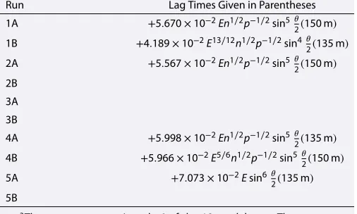
[image:9.612.37.567.548.727.2]Table 5.Model Terms Identified as Ring Current Losses Due to Flowouta
Run Lag Times Given in Parentheses
1A +5.670×10⁻²En1∕2p−1∕2sin5𝜃 2(150m) 1B +4.189×10⁻²E13∕12n1∕2p−1∕2sin4𝜃
2(135m) 2A +5.567×10⁻²En1∕2p−1∕2sin5𝜃
2(150m) 2B
3A
3B
4A +5.998×10⁻²En1∕2p−1∕2sin5𝜃 2(135m) 4B +5.966×10⁻²E5∕6n1∕2p−1∕2sin5𝜃
2(150m)
5A +7.073×10⁻²Esin6𝜃
2(135m) 5B
aThese terms appear in only 6 of the 10 model runs. They represent equation (6e).
They each containΔ√p, have lags of 10 min or less, and the coefficients are all positive. All three of the terms from a model run, added together, represent equation (6b).
The 0 min lag represents Chapman-Ferraro (magnetopause) currents on the dayside magnetosphere, since this is the time when a particular element of the solar wind reaches Earth. Alongside the expectedΔ√p parameter, the 0 lag terms consistently contain the electric field,E, raised to the power 1∕3to 1∕2. This is not surprising because the magnetopause is up to 1REcloser to Earth when the IMF is oriented in theYZplane
(i.e., perpendicular to the solar wind velocity) [Dusik et al., 2010].
In some of the runspappears with a small positive power in the 0 lag result, indicating thatΔ√pmight not be ideal, with the true power ofpbeing slightly larger than 0.5. Three of the other runs containn−1∕6p1∕4,
which can be written asp1∕12v1∕3, so they contain the same small-powered pressure factor, with an
addi-tional velocity contribution. Although it appears thatvhas a greater contribution in these terms, the power of E(=vBT)is smaller, and it is actually the contribution fromBTthat is less significant.
The 10 min lag terms are very different from the 0 min lags. They contain two factors,n3∕2andp−2. The 10 min
lags correspond to the time it takes the solar wind to pass the Earth and begin to apply pressure to the magne-totail. It is tempting to associaten3∕2with an enhanced plasma sheet density, andp−2with a cross-tail current
that moves toward or away from Earth with the varying solar wind dynamic pressure, an effect suggested byMcPherron and O’Brien[2001] to affectDst. However, the two factors when combined are approximately equivalent to a large inverse power of velocity (v−4), meaning that this term is significantly more important
when the solar wind velocity is small. It remains a possibility that≈10min errors in the time shifting of OMNI data during periods of low solar wind velocity could be responsible for the 10 min lag terms, but if the time shifting is correct, then the above explanation is plausible. The 5 min lag terms are simply a combination of the 0 lags and 10 min lags.
7.3. Open Magnetic Flux
Two to three terms resembling the well-known coupling functions are present in each model run. They are listed in Table 3, and represent equation (6c). Some examples of previously suggested coupling functions are given in section 5 for comparison. Each of these were available, among the 4.8 million candidate terms, to the NARMAX code, with lags of up to 4 h. The NARMAX selected terms all have negative coefficients, and lags between 20 and 30 min. The functions closely resemble the rate of dayside merging of solar wind and geomagnetic field [see, e.g.,Vasyli¯unas, 2006]. All of the properties match expected changes inSYM-Hfrom the piling up of open magnetic flux in the magnetotail and the corresponding enhancement of the cross-tail current, which results in an increase of−SYM-H.
Terms with 20 min lags are present in every model run. They are of the form−Ex1px2sinx3 𝜃
2, wherex1=9∕12
to 11∕12,x2=3∕12to 5∕12, andx3=4to 5. The coupling function ofTemerin and Li[2006] can be
writ-tenET&L=Ep1∕2sin6𝜃2, so the 20 min lag terms are equivalent toE 5∕6
T&L. At longer lag times the sameEand
Figure 2.Schematic showing the physical processes identified in the NARMAX model terms, with the typical lag times. (i) An element of solar wind arrives at the dayside magnetopause. (ii) The IMF in that element merges with the geomagnetic field, while the solar wind dynamic pressure temporarily contributes toSYM-Hvia Chapman-Ferraro currents. (iii) Open geomagnetic field piles up in the magnetotail, enhancing the tail current and
−SYM-H. (iv) The open geomagnetic field has diffused through the magnetotail and begins to reconnect. (v) Charged particles are injected into the ring current, as the magnetotail dipolarizes and the cross-tail current decays. Energy is lost from the magnetosphere in the plasmoid traveling downwind and by ionospheric Joule heating. (vi) An hour after the ring current particles are injected from the magnetotail they reach the dayside, where those on pseudotrapped orbits escape through the magnetopause, causing−SYM-Hto decay.
pronounced than in the 10 min lag pres-sure terms in the previous section, and it is unclear if they are both a product of errors in the time shifting of OMNI data at low solar wind speeds.
7.4. Tail Reconnection and Particle Injection Typically around an hour after open magnetic flux enters the magnetotail, it has diffused through the tail to the point of reconnection. As the magnetic field dipolarizes following recon-nection, charged particles are simultaneously injected into the ring current. This process is represented by equation (6d), and the associ-ated model terms are given in Table 4. Although the NARMAX model describes steady, continu-ous reconnection, in nature it tends to be bursty. The piling up of magnetic flux in the tail cor-responds to the substorm growth phase, and the bursts of reconnection and particle injec-tion are substorm expansion. The timing of substorms is very difficult, if not impossible, to predict using solar wind parameters alone, and it is not clear how much the model repre-sents a smoothed time average over the bursty events or how much it represents steady tail reconnection occurring between the substorms. The increase in ring current particles enhances −SYM-H, whereas the loss of magnetic flux in the tail reduces −SYM-H. According to Siscoe and Petschek[1997], the contribution toSYM-H from energy in the ring current is twice that of energy stored in the magnetotail. This means that if all of the energy stored in the magne-totail is converted to ring current energy, then −SYM-H should increase. The positive sign of the terms indicate that most of the energy is lost to other processes. This is in agreement with a statistical study of the substorm expan-sion energy budget byTanskanen[2002], which gives figures of 30% for each of charged particle precipitation, Joule heating, and the escaping plasmoid, with the remaining 10% going to the ring current.
The functions identified with tail reconnec-tion appear to be the geometric means of the near-instantaneousSYM-H∗and the dayside magnetic field merging delayed by between 60 and 120 min. It
could be that these terms are the closest approximations, among the 4.8 million candidates, to a geometric combination of the merged flux reaching the tail reconnection point (70 to 110 min after merging on the day-side) and the instantaneous magnetic pressure in the tail, which is driving the reconnection. AlthoughSYM-H∗
7.5. Flowout
Terms in the NARMAX results identified as flowout (Table 5) are the least significant among the coupling pro-cesses. They are only present in the results of 6 out of 10 runs. The functions superficially resemble the rate of magnetic field merging, but all except one depend only on the IMF and can be written asBTsin5𝜃
2. The
lag times of 135 to 150 min are around an hour longer than the lag for particle injection into the ring cur-rent, which is consistent with the typical time it takes the bulk of injected particles to drift from the nightside injection region to the dayside magnetopause.
The difficulty in finding these functions with NARMAX could be because there are simply no good candidate terms that accurately describe the flowout rate. The actual flowout rate is expected to depend on the current location of the magnetopause and the 1 h lagged charged particle injection rate. However, as we have seen, the rates of tail reconnection and particle injection will depend onSYM-H∗at that time (1 h ago) and
day-side merging 90 min before that. Allowing multiple different lags of the solar wind parameters in each term results in far too many candidates than can be processed by the NARMAX code in any reasonable amount of time.
7.6. Division of Energy Between Loss Processes
Over long timescales (i.e., the whole data set), approximately 49% of the overall loss ofSYM-Hin the NARMAX model is due to the terms identified with tail reconnection, 34% to particle precipitation, and the remaining 17% from terms that appear to represent flowout. These losses are ofSYM-H, not energy, and when estimating the transfer of energy, the factor of 2 in equation (2) must be taken into account. The 49% loss inSYM-Hfrom tail reconnection translates to a 74.5% loss in energy, primarily to the escaping plasmoid and Joule heating. This is roughly consistent withIeda et al.[1998] andKamide and Baumjohann[1993], who suggest approximate equipartition of energy between the ring current, the escaping plasmoid, and ionospheric Joule heating. Of the remaining 25.5% of the energy that enters the ring current, around a third (8.5%) is lost via the flowout terms and two thirds (17%) to particle precipitation. The loss due to particle precipitation is in line with a previous estimate of 12% byWang et al.[2014].
7.7. Variability Between Model Runs
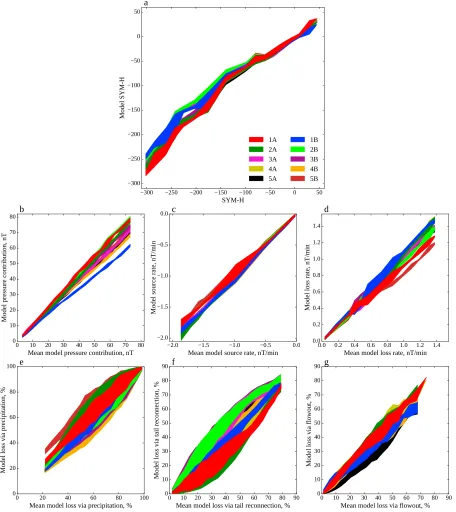
To estimate the robustness of the results, the NARMAX model was run 10 times, each time varying the selection of input data (see section 3). Figure 3 shows the relative magnitudes of the model terms for each model run, along with the overall accuracy of each model in reproducing the observedSYM-H. The data used in Figure 3 are from 17 March 2000 to 9 May 2000, a period that was entirely excluded from the NARMAX algorithm in all of the model runs.
Figure 3a shows the ability of the model to predictSYM-Husing only the measured solar wind parameters. The modelSYM-His calculated in an iterative manner, using previousmodelvalues ofSYM-Hwith actual solar wind measurements, in the NARMAX model terms (Table 1). In Figure 3a the model samples are binned according to theSYM-Hobservations, with no less than 12 samples per bin. The colored patches represent the central 50% of the model samples in each bin. There is little difference between each of the models, especially at small to moderate−SYM-Hwhere there are many samples. During these months in the spring of 2000, the mod-els appear to systematically underestimate larger−SYM-H, but most of these samples occur in the declining phase of a single storm on 6 April 2000 (see Figure 4).
Figure 3b shows the variation in the magnetopause current terms of each model run. Run 1B produces a slightly smaller estimate of the magnetopause current contribution toSYM-H, but the narrow distributions (thin patches) indicate that the differences between model runs is primarily a scaling factor.
Figures 3c and 3d show the overall source and loss terms. The source terms are those associated with the magnetic field merging on the dayside (Table 3), while the loss terms include particle precipitation (corresponding to𝜏in equation (6)), tail reconnection (Table 4), and flowout (Table 5). The individual loss processes are broken down in Figures 3e–3g.
Figure 3.The variation between model runs. (a) The modelSYM-Hfrom each run against the correspondingSYM-Hobservations. The samples are binned according to observedSYM-H, with a minimum of 12 samples per bin. The colored patches span the25th to the75th percentiles, i.e., half of the model samples are within the patches. For Figures 3b–3g, direct observations of the parameters are not possible, so the mean value from the model runs is used for thexaxes. (b) The contribution toSYM-Hfrom magnetopause currents (see Table 2). (c) The magnitude of the source terms (see Table 3) and (d) the loss terms. (e–g) The loss rates are broken down, corresponding to losses via particle precipitation (𝜏in equation (6)), tail reconnection (Table 4), and flowout (Table 5), respectively.
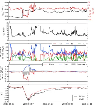
Figure 4.Results from the first run of the NARMAX model (run 1A), for the geomagnetic storm beginning 6 April 2000. (a) The prevailing solar wind velocity and interplanetary magnetic field in theZ(GSM) direction. (b) The effective exponential lifetime ofSYM-H, in hours. (c) The sizes of the loss terms are compared, where PP is particle precipitation/ charge exchange, FO is flowout, and Tail is the loss ofSYM-Hfrom magnetotail reconnection. (d) The total source (negative terms) and loss (positive terms) are compared. (e) A comparison of the measuredSYM-Hvalues and NARMAX-predicted values. Here the model results are calculated using only the solar wind measurements, and preceding modelSYM-H, without any reference to measured values ofSYM-H.
8. Case Studies
Figures 4–6 show the results of NARMAX model run 1A during three geomagnetic storms, beginning on 6 April 2000, 24 April 2000, and 20 November 2003, respectively. Figures 4a, 5a, and 6a show the prevailing solar wind velocity and southward component of the IMF during the storms. The effective exponential decay time constant ofSYM-H∗,𝜏
eff, given in Figures 4b, 5b, and 6b, is based on the totalSYM-H∗loss rate,
includ-ing flowout, tail reconnection, and the purely exponential decay term of equation (6a). A breakdown of the percentage losses from each of these processes is given in Figures 4c, 5c, and 6c.
Figures 4d, 5d, and 6d compare the magnitude of the source term with the combined loss term. The source is the merging of magnetic field on the dayside−aΔΦd(equation (6c)) and has units of nT/min. The shaded region shows the overall rate of change ofSYM-H∗, i.e., the combination of source and loss, also in nT/min.
Figures 4e, 5e, and 6e show the measured value ofSYM-H(black) and the model values (red). The model results are calculated iteratively using the NARMAX model terms to calculate the next value ofSYM-Hbased on the previous model value and solar wind data. The iteration begins at least 4 h prior to the time period of interest, to allow it to converge and become independent of the starting value.
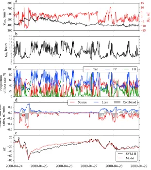
Figure 5.As in Figure 4 but for the storm beginning 24 April 2000.
The losses ofSYM-Hincrease much more slowly. Initially, and while the storm is being driven by the solar wind, the losses are mostly incurred in the tail reconnection (see Figures 4c, 5c, and 6c). During this time a large proportion of theSYM-Hvalue comes from the distorted magnetotail. As the open magnetic field in the tail reconnects, most of the energy is lost to Joule heating, particle precipitation, and the plasmoid, and therefore the magnetotail contribution toSYM-His not wholly replaced by the increase in ring current. In the declining phases of the storms the losses are mostly due to the idealized loss term, (equation (6a)) which is assumed to primarily represent charge exchange (particle precipitation) losses. These features, and the over-all loss rate, match those given by the numerical model ofKozyra and Liemohn[2003]. It is clear from Figure 5d that the NARMAX model is capable of reproducing the smallest of changes seen inSYM-H, but the longer-term decay following the storm is not as accurate. While the model makes good use of high-resolution solar wind data, it lacks the complicated physics and wave-particle interactions that control acceleration and loss inside the magnetosphere.
9. Performance of the Model
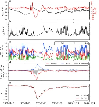
Figure 6.As in Figure 4 but for the storm beginning 20 November 2003.
because it has been excluded from the data used to produce all four of the models. AlthoughTemerin and Li [2006] provide an updated version of theTemerin et al.[1472] model, it is not used here because it is trained on the data from this test period, giving it an unfair advantage. The present model compares favorably with the others, although it may be at a disadvantage due to the high time resolution ofSYM-H, which could naturally lead to higher RMSE than the low-resolutionDstindex. The model ofTemerin et al.[1472] is by far the most complicated of the four models. It performs very well overall but poorly for the large storm of the third case study (20 November 2003).
Table 6.A Performance Comparison ofSYM-HandDstModelsa
Model Parameter RMSE (nT) Correlation Coefficient
Average Over the Three Case Studies
This study, run 1A SYM-H 20.4 0.952
Burton et al.[1975] Dst 38.1 0.894
Boynton et al.[2011] Dst 19.3 0.966
Temerin et al.[1472] Dst 43.2 0.885
17 March 2000 to 9 May 2000
This study, run 1A SYM-H 11.0 0.959
Burton et al.[1975] Dst 14.5 0.891
Boynton et al.[2011] Dst 11.5 0.948
Temerin et al.[1472] Dst 9.26 0.961
[image:16.612.173.575.571.726.2]10. Summary
There are some limitations in the method and results of the models presented in this study. First, the NARMAX algorithm can only select from a finite set of candidate predictors. Some coupling processes might not be well represented by any of the available choices. This is likely the case with the model flowout terms. The actual flowout rate depends on multiple different lags of solar wind parameters; these determine the density of ring current particles and control the dayside loss rate of those particles by altering the location of the magne-topause. Second, the maximum lag time in the models is 4 h. Some magnetospheric processes take longer than this. For example, high-energy (MeV) particles respond with 5 to 40 h delays to solar wind enhancements [Li et al., 2005]. These particles are energized in different processes to the lower energy particles that dominate the ring current. However, their populations are too small to significantly affectSYM-H.
Despite these limitations, the NARMAX algorithm has produced models that accurately reproduceSYM-H, while quantifying several of the individual coupling processes and providing their lag times. According to the NARMAX models, the lag time between the merging of the IMF and geomagnetic field and the increase in tail currents from the stretched magnetotail is 20 to 30 min. The lag time from dayside merging to magnetotail reconnection is 60 to 120 min. These times match the impulse response of theALindex to changes in solar windvBS, which is observed to have two peaks at 20 min and 60 min [Bargatze et al., 1985]. Note that although
tail reconnection causes a decay in−SYM-H, this is not the case with theALindex, which responds positively to substorm expansion.
It is difficult to say which of the model runs will provide the truest representation of any particular geomag-netic storm. There are slight variations in the performance of the models depending on the particular event. The most significant difference between the models is the division of losses between the different loss mech-anisms. Any of the models that include the flowout loss term (i.e., models 1A, 1B, 2A, 4A, 4B, or 5A) should be equally valid, within the errors of this investigation. We would recommend using model 1A, for ease of compar-ison with the results of this study and because it provides values ofSYM-Hslightly closer to the measurements during the largest storms.
The models provide empirical evidence for the theory ofVasyli¯unas[2006], namely, that the negative swings inDstandSYM-H, which are described by the well-known coupling functions, are first an observation of the open geomagnetic field piling up in the magnetotail and enhancing cross-tail currents. When particles are injected on the nightside during tail reconnection,−SYM-Hdecays. This is because the loss of−SYM-Hfrom the dipolarization of the geomagnetic tail is greater than the gain in−SYM-Hfrom the particle injection. AlthoughVasyli¯unas[2006] expected the effects of dipolarization and injection to almost cancel, this result is in agreement with other studies [Iyemori and Rao, 1996;Siscoe and Petschek, 1997].
References
Bargatze, L. F., D. N. Baker, R. L. McPherron, and E. W. Hones (1985), Magnetospheric impulse response for many levels of geomagnetic activity,J. Geophys. Res.,90(A7), 6387–6394.
Billings, S. A., and H. L. Wei (2005), The wavelet NARMAX representation: A hybrid model structure combining polynomial models with multiresolution wavelet decompositions,Int. J. Syst. Sci.,36, 137–152.
Billings, S. A. (2013),Nonlinear System Identification: NARMAX Methods in the Time, Frequency, and Spatio-Temporal Domains, Wiley, Chichester, U. K., doi:10.1002/9781118535561.
Boynton, R. J., M. A. Balikhin, S. A. Billings, A. S. Sharma, and O. A. Amariutei (2011), Data derived NARMAX Dst model,Ann. Geophys.,29, 965–971, doi:10.5194/angeo-29-965-2011.
Boynton, R. J., M. A. Balikhin, S. A. Billings, H. L. Wei, and N. Ganushkina (2011), Using the NARMAX OLS-ERR algorithm to obtain the most influential coupling functions that affect the evolution of the magnetosphere,J. Geophys. Res.,116, A05218, doi:10.1029/2010JA015505. Burton, R. K., R. L. McPherron, and C. T. Russell (1975), An empirical relationship between interplanetary conditions and Dst,J. Geophys. Res.,
80, 4204–4214.
Dessler, A. J., and E. N. Parker (1959), Hydromagnetic theory of magnetic storms,J. Geophys. Res.,64, 2239–2259.
Dusik, S., G. Granko, J. Safrankova, Z. Nemecek, and K. Jelinek (2010), IMF cone angle control of the magnetopause location: Statistical study, Geophys. Res. Lett.,37, L19103, doi:10.1029/2010GL044965.
Hoffmann, W. (1989), Iterative algorithms for Gram-Schmidt orthogonalization,Computing,41(4), 335–348.
Hong, X., and C. J. Harris (2001), Nonlinear model selection structure detection using optimum experimental design and orthogonal least squares,IEEE Trans. Neural Networks,12(2), 435–439.
Ieda, A., S. Machida, T. Mukai, Y. Saito, T. Yamamoto, A. Nishida, T. Terasawa, and S. Kokubun (1998), Statistical analysis of the plasmoid evolution with Geotail observations,J. Geophys. Res.,103(A3), 4453–4465.
Iyemori, T., and D. R. K. Rao (1996), Decay of the Dst field of geomagnetic disturbance after substorm onset and its implication to storm–substorm relation,Ann. Geophys.,14, 608–618.
Kamide, Y., and W. Baumjohann (1993),Magnetosphere-Ionosphere Coupling, Springer-Verlag, New York. Kan, J. R., and L. C. Lee (1979), Energy coupling and the solar wind dynamo,Geophys. Res. Lett.,6, 577–580.
Acknowledgments