In the agricultural and rural policy making, the levels and the distribution of farmers’ incomes are of a particular importance. Thus, many countries have typically framed the income objectives of agricultural policies in terms of the distribution or equity (OECD 1998; Moreddu 2011). Along these lines, agricultural policy instruments such as the price support and di-rect payments have an effect on the farmers’ income and income distribution. In particular, most direct payment instruments within agricultural policy have at least partially shifted the objective of income redis-tribution towards the neediest parts of the farming population (Mann 2005). In most European countries, the importance of direct payments for incomes of farm households increased considerable over time while market supports were heavily reduced within the last decades due to policy reforms.
However, the analysis of the effects of different income sources on the income distribution within the farm population as well as the dynamics in these relationships observed over time has received little attention so far. Particularly, the research about the impact of specific direct payment programmes on income inequality is scarce. The existing studies of the distributional effects of policy changes in European agriculture show mixed results. For instance, Keeney (2000) found that due to an increasing share of support payments in the total farm income, Irish farm income inequality decreased between 1991 and 1996 (pre- to post-MacSharry reform). Whereas the programmes that target farmers in less favoured areas reduced
income inequality, the per hectare arable payments increased it. By comparing the pre-support with the post-support Scottish farm income, Allanson (2005) shows that the measures of the MacSharry reform progressively support farmers with the negative or low pre-support incomes. Schmid et al. (2006) show that the less-favoured area payments have had only a minor effect on the absolute income inequality in Austria, but that direct payments and agri-environmental payments increased the absolute income inequality. Results of von Witzke and Noleppa (2007) show that direct payments significantly contribute to income inequality in German agriculture.
Based on this background, the goal of this paper is to measure the effect of Swiss agricultural policy reforms on the distribution of income within the farm population. Switzerland serves as a good case study for European countries to analyse the effects of the changing farm-level supports on the income distribu-tion. Swiss agricultural policy faced a dramatic shift from the market-based support to direct payments and most of the direct payment instruments available to Swiss farmers are very similar to those applied or thought to be introduced by the European Union (cp. section 2 and see e.g. Mann 2003). Regarding the specific case of Switzerland, there exist studies that deal with income distribution within the Swiss population at large (e.g. Gerfin 1994; Zürcher 2004; Engler 2010), but there is little research dealing with the impact of various income sources on the overall income inequality (e.g. Flückiger and Silber 1995).
The distributional effects of agricultural policy reforms
in Switzerland
Nadja El Benni
1, Robert Finger
1, Stefan Mann
2, Bernard Lehmann
11
Swiss Federal Institute of Technology Zurich (ETH Zurich), Zurich, Switzerland
2
Research Station Agroscope Reckenholz-Tänikon ART, Ettenhausen, Switzerland
Abstract: Th is paper analyses the eff ects of Swiss agricultural policy reforms and the eff ects of farm income, off -farm in-come and direct payments on the distribution of the farm household inin-come. To this end, the farm-level inin-come records from the FADN data for the period 1990–2009 are used to calculate Gini coeffi cients and Gini elasticities. Bootstrap sam-pling procedures are applied to test for signifi cant diff erences of the estimated parameters over time. Th e Gini coeffi cients estimated in our analysis show that the household income inequality in Swiss agriculture only slightly increased from 0.21 to 0.24, but the farm income inequality strongly increased from 0.27 to 0.38 in the considered period. We fi nd furthermore that increasing off -farm incomes and direct payments would decrease the household income inequality. Especially direct payments that support farmers producing under adverse production conditions in the hill and mountain regions have found to be well targeted and thus contribute to the reductions in income inequality in agriculture.
Most importantly, income inequality in Swiss agri-culture has not been addressed so far.
Besides the specific contribution for the Swiss case, our analysis expands the existing studies also from the methodological points of view. To our knowledge, this is the first paper that uses the farm-level data over a range of twenty years (including two main re-form steps) to measure the effects of different direct payment programmes on the income distribution. Furthermore, we use bootstrap procedures to test for significant differences over time. To account for the real income situation of farmers, we expand the farm-income perspective and analyse the effect of policy changes with regard to the total household income, including farm income and off-farm income1. In the
first step, the effect of agricultural policy reforms on the distribution of household income is analysed. In the second step, a more specific analysis is under-taken to measure the effect of eleven direct payment programmes on the household income distribution, including the general and ecological payments as well as the animal welfare payments and the payments that support farmers producing under adverse produc-tion condiproduc-tions. Thus, marginal effects how specific direct payments contribute to income inequality in agriculture are estimated. The results may be used by the policy makers to examine numerically the distribu-tional effects of the past and proposed policy changes.
This paper is structured as follows. In section 2, the main developments of Swiss agricultural policy between 1990 and 2009 are briefly described. The data and methods used in this paper are presented in the 3rd section. In the 4th section, the marginal effects of
agricultural policy reforms and single direct payment programmes on the household income distribution are explored. Furthermore, we analyse how the changes in the importance and distribution of different income sources affect the changes in the household income distribution. The analyses investigate the hypothesis that the changes in income inequality can be attrib-uted to the agricultural policy reforms. Section 5 summarizes and discusses the results.
DIRECT PAYMENTS AND THE AGRICULTURAL POLICY REFORMS IN SWITZERLAND
Roughly two main steps within the reform process of Swiss agricultural policy can be distinguished, the
first being in 1992 and the second in 1999. With each reform step, the market support was reduced and the farm-level based subsidies were introduced as compensation. Pre-reform subsidies that were already available to the farmers prior to 1992 included the payments provided per farm household. Furthermore, the area-based and animal-head based payments were given to farmers producing under adverse production conditions mainly in the hill and mountain regions of Switzerland. The policy goal followed by these payments was the support of farmers that were not able to earn an appropriate income from marketable goods. The support in the frame of farm household payments ended in the late 1990s. With the first policy reform in 1992, decoupled direct payments were introduced without geographical restrictions. Area-based and animal unit based payments were introduced for all farmers. Furthermore, farmers could voluntarily apply to agri-environmental schemes that aim at promoting the environmental-friendly pro-duction systems. These agri-environmental schemes included payments for the extensive crop production and ecological compensation areas.
With the next reform cycle starting in 1999, a new direct payment system was introduced dividing sup-port payments into the general and the ecological direct payments. The general direct payments were based on a cross-compliance approach. Thus, farmers had to comply with the baseline criteria regarding the environmental and animal friendly production, with the most restrictive being the set-aside of seven percent of their farmland as the ecological compensa-tory area (Mann 2003). As previously, farmers could apply voluntarily to the ecological direct payment programmes.
Since 1999, no considerable changes in the direct payment system were made. One exception is the in-troduction of a new performance-oriented ecological direct payment programme in 2001, aiming at enhanc-ing and increasenhanc-ing the biodiversity on cultural land. Currently, the general direct payments constitute most of the financial support (79% in 2009 (FOA 2010)) and include the animal unit and area-based payments to farmers within all regions and the additional payments for farmers producing under adverse production condi-tions in the hilly and mountainous regions. Ecological direct payments include the payments for the extensive crop production, the ecological compensation areas and the eco-quality. Furthermore, two animal welfare programmes are available2.
1See Hill (1999) for detailed discussions on the issue of income measures for the agricultural community.
Beside direct payments, the production of oil seeds, legumes, fibre crops, potato seed, cereals and fodder plants are supported by the arable payments. While these payments were adapted over the last two dec-ades, they are paid with the aim to enrich the crop rotation and for the food security reasons. This sup-port measure falls under the aforementioned cross compliance conditions as well.
METHOD AND DATA
Gini decomposition by income source
The Gini coefficient of inequality is a commonly used measure in the income inequality research (Flückiger and Silber 1995). For non-negative incomes, the Gini coefficient measures the relative income inequality and ranges between 0 and 1. The Gini coefficient equals 0 if the household income is totally equally distributed, and it increases the more unequal the income distribution becomes. To estimate the Gini coefficient G, the household income Y is assumed to be a random variable, distributed with the mean μ over the farm population. With F(Y) denoting the cumulative distribution function of the household income and cov(.) the covariance, Stuart (1954) shows that the Gini coefficient of relative income inequality can be written as follows:
2cov Y,F(Y)
G (1)
To measure the effect of different income sources on the aggregated income inequality, the Gini de-composition approach of Fei et al. (1978) and Pyatt et al. (1980) extended by Lerman and Yitzhaki (1985) is applied. Using this method, the total household income is defined as the sum of incomes from k dif-ferent sources Ykwith F(Yk) denoting the cumulative distribution function of the income source under consideration. The decomposed Gini coefficient can be written as follows:
2cov
, ( )
)) ( , cov ) ( , cov ( 1
k k k k Kk k k
k y F Y
Y F y Y F y
G (2)
K k k k kG SR G
1
(2a)
Th e Gini correlation Rk ranges between –1 and +1 and it is defi ned as the covariance between the kth compo-nent income and the cumulative distribution of total income, divided by the covariance between the kth
component income with its own cumulative distribu-tion (Pyatt et al. 1980). If the income of the kth income
source increases (decreases) with increasing the total income, Rk is positive (negative), and if Rk equals 0 the income source is a constant not contributing to the total income inequality. Gk is the Gini coefficient of the kth income source, showing how the income
from the specific income source is distributed within the population. The share of the kth income source
on total income is given by Sk. Rk times Gk yields the concentration ratio or the Pseudo-Gini coefficient Ck, which measures how the income from each source is transferred across the population ranked with respect to the level of the total income received:
k
k k k k k k k k Y F y Y F Y Y F y Y F y C
2cov , ( ) 2cov , ( )
) ( , cov ) ( ,
cov (3)
The concentration ratio is 0 if all income groups receive an equal amount of income of the given in-come component (Pyatt et al. 1980); it is negative if the income from a specific source accrues mainly to the households in the lower tail of the distribution of the total income; and it is positive, if the richer households receive a large proportion of the income from the specific income component. The concen-tration ratio that is larger than the Gini coefficient of the aggregate income proves that the income component in question has had an unequalising ef-fect on the observed aggregate income distribution (Keeney 2000).
The marginal effects of different income sources on income inequality
To measure the effect of a specific income compo-nent on the aggregated income inequality, the Gini elasticity is calculated as proposed by Lerman and Yithzaki (1985). The Gini elasticity gives information on how the income distribution would change with a marginal percentage change in the mean income of the specific income component. By assuming that the ratio between the total income distribution and the income source remains undisturbed, the rate of change of the Gini coefficient is derived as follows:
» ¼ º « ¬ ª P P P u P
K 1 (C G)
G d dG G k k k k
k (4)
concentration coefficient and the Gini coefficients coincide (Podder 1995; Keeney 2000)3.
In order to test if changes of the Gini coefficients, the Pseudo-Gini coefficients and the Gini elastici-ties over time are statistically significant, we use the non-parametric bootstrap (see DiCiccio and Efron 1996, for details). To this end, the above described point estimates are estimated for 1000 data replicates that are generated by sampling with the replacement from each of the initial datasets. Thus, the estimation procedure4 is replicated for the 1000 newly generated
datasets. This leads to 1000 estimates for the Gini coefficients, the Gini elasticities and the Pseudo-Ginis for each year, which are used to construct 95% confidence intervals by discarding the 2.5% small-est and largsmall-est point small-estimates, respectively. These confidence intervals are used to test for significant differences between different years, though we are aware that the tests based on overlapping confidence intervals are a very conservative way of hypothesis testing (Schenker and Gentleman 2001). All statistical analyses are conducted with the statistical language and environment R (R Development Core Team 2011).
Causes of the change in income inequality
To analyse if changes in the share or changes in the distribution of the different income sources are the driving force for the overall inequality changes over time, the approach of Podder and Chatterjee (2002) is used. Therefore, the change of the Gini coefficient over time ΔG is divided into a share effect (SE) and a concentration effect (CE):
ΔGt≈ SE + CE (5)
The change in the aggregated Gini coefficient from the period t – 1 to the period t is given by ΔGt = Gt – Gt–1. Changes in the Gini coefficient can be attributed to a change in the share of the kth income component in the total income ΔSk,t = Sk,t – Sk,t–1
between the period t – 1 and t and to the change in the concentration coefficient ΔCk,t = Ck,t – Ck,t–1 over
the same period. Hence, the changes in the share of a specific income component as well as the changes in the distribution of an income component over the range of the total income affect the change of the Gini coefficient. The difference between two time periods can be measured with respect to the base period or with respect to the terminal period, which would lead to a different result. Therefore, Podder and Chatterjee (2002) suggest the following approximation of the share and the concentration effect:
t k K
k
t k t k
S C C
SE ,
1
1 , ,
2 u'
¦
(6)t k K
k
t k t k
C S S
CE ,
1
1 , ,
2 u'
¦
(7)According to Eq. 6, the share effect SE of all income components is approximated by the sum of the changes in the shares of the different income components from one year to another weighted by their average changes in the concentration coefficient over the same time period (and vice versa for the concentration effect as shown in Eq. 7).
Data
The farm-level income data of the Swiss National Farm accounting Network (FADN) over the period 1990 to 2009 are used. The total household income is defined as the gross household income minus the total production costs, labour costs and interest on debt and land and it is decomposed into the off-farm income, the farm income, and the income from (dif-ferent) direct payments. For the analyses, the sample of the FADN farm households is weighted based on the farm size, the farm production system, and region5. Since the dataset contains some extreme
values, the 2.5% households at the top and the bot-tom end of the total household income distribution were excluded from the analysis. The final dataset includes in average 3460 farm operations per year, representing (after weighting) a farm population of the average 52 180 farms per year.
3In the presence of negative incomes, the Gini coefficient here presented may exceed unity and the estimates of the elasticities are analytically correct but biased upwards (Boisvert and Ranney 1990). Even if methods exist to estimate here presented Gini coefficients that account for negative incomes (Chen et al. 1982), these coefficients cannot be decomposed by here presented income source (Boisvert and Ranney 1990) and their interpretation is difficult (van de Ven 2001). Hence, by using the here presented here presented Gini decomposition approach, the marginal effects of different income components on income inequality can be biased upwards. Nevertheless, the qualitative policy implications remain by choosing this approach (Boisvert and Ranney 1990).
4This also includes trimming and weighting for each dataset.
RESULTS
This section presents the results of the Gini de-composition for the total household income. In the first step, the effects of the off-farm income, the farm income and direct payments (in general) on the household income inequality are estimated. Second, we analyse if the changes in the share or in the dis-tribution of the different income components led to the changes in the Gini coefficient of the total household income.
In addition, we measure the effects of single direct payments schemes on the Gini coefficient of house-hold income and its changes over time.
The effect of agricultural policy reforms on the total household income inequality
The contribution of farm income, off-farm income and direct payments to the household income inequality
In this section, we investigate how the agricultural policy reforms, i.e. the change from market support to direct payments, had affected the distribution of household income within the Swiss farm
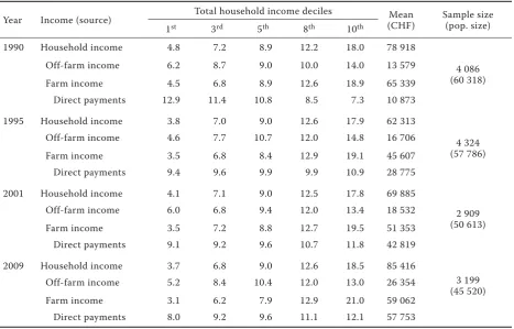
popula-tion. Table 1 shows the share of the total household income, the farm and off-farm income, and the in-come from direct payments by the selected total household income decile for the years 1990, 1995, 2001 and 2009. More precisely, the farms were ranked by decile according to their total household income level. The mean of each income decile was divided by the sum of the total household income, i.e. the sector household income. The same was done for all other income sources. For instance, the mean direct payment income in the first household income decile was divided by the sum of all direct payment given to the sector. The years were chosen to represent the pre-reform (1990), the first reform (1995), the second reform (2001) and the current (2009) situation.
The share of the total sector household income received by households in the 10th decile (i.e. the
households with the highest incomes) is about 18%, while the share received by the 1st decile (i.e. the
households with the lowest incomes) is about 5%. Farms with higher household incomes generate more of the sectors’ off-farm income than the farmers in the lower household income decile. Also, the farm income is mainly generated by farmers in the high-est income decile. In 1990, about 19% of the sectors farm income was generated by the 10th income decile,
[image:5.595.65.533.451.750.2]and only 4.5% by the first income decile. In 2009,
Table 1. Income shares of different income sources by deciles of total household income
Year Income (source) Total household income deciles Mean (CHF)
Sample size (pop. size)
1st 3rd 5th 8th 10th
1990 Household income 4.8 7.2 8.9 12.2 18.0 78 918
4 086 (60 318)
Off-farm income 6.2 8.7 9.0 10.0 14.0 13 579
Farm income 4.5 6.8 8.9 12.6 18.9 65 339
Direct payments 12.9 11.4 10.8 8.5 7.3 10 873
1995 Household income 3.8 7.0 9.0 12.6 17.9 62 313
4 324 (57 786)
Off-farm income 4.6 7.7 10.7 12.0 14.8 16 706
Farm income 3.5 6.8 8.4 12.9 19.1 45 607
Direct payments 9.4 9.6 9.9 9.9 10.9 28 775
2001 Household income 4.1 7.1 9.0 12.5 17.8 69 885
2 909 (50 613)
Off-farm income 6.0 6.8 9.4 12.0 13.4 18 532
Farm income 3.5 7.2 8.8 12.7 19.5 51 353
Direct payments 9.1 9.2 9.6 10.7 11.8 42 819
2009 Household income 3.7 6.8 9.0 12.6 18.5 85 416
3 199 (45 520)
Off-farm income 5.2 8.4 10.4 12.0 13.0 26 354
Farm income 3.1 6.2 7.9 12.9 21.0 59 062
Direct payments 8.0 9.2 9.6 11.1 12.1 57 753
the 10th household income decile generated 21% of
the sectors’ farm income and the first income decile generated only 3%.
The distribution of income from direct payments over the total household income deciles (4th row in
each subsection of Table 1) reveals some interesting changes over time. In 1990, households in the lowest income decile received about 13% of the total govern-mental farm-level support, while farmers in the highest income decile received only 7% of the total support. In contrast, farmers in the first household income decile received only 8% of the total governmental support in 2009, while farmers in the highest decile received 12% of the total support. Thus, direct payments were re-distributed across the farm population.
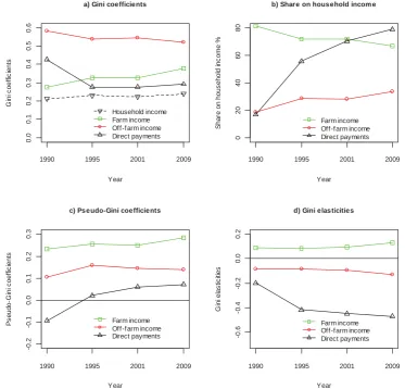
Figure 1 shows the decomposition results for the total household income inequality calculated accord-ing to the equations 1 to 4. Figure 1b shows that direct payments became a very important income source for farmers after the agricultural policy reform in 1992. Since 2001, direct payments are even higher than the farm income. Hence, part of the direct payments is used by farmers to cover the costs of production. Also
the importance of the off-farm income increased over time, making up about 33% of the total household income in 2009.
The Gini coefficients (Figure 1a) show that the farm income is less equally distributed than the household income. It shows, furthermore, that the farm income inequality strongly increased (the Gini coefficient was 0.27 in 1990 and 0.38 in 2009) while the household income inequality only slightly increased over time (the Gini coefficient was 0.21 in 1990 and 0.24 in 2009). In general, the off-farm income is the most unequally distributed income source, even if inequality decreased over the here considered time period. This might be explained by the differences in the off-farm employment opportunities in e.g. different regions and different needs of farmers to earn money off the farm. With the first agricultural policy reform in 1992, the area-based direct payments were introduced and were made available to all farmers without geographical restrictions. This led to a wide spread of the farm-level support within the Swiss farm population and decreased the Gini coefficient considerably (from 0.43 in 1990 to 0.29 in 2009).
0.0
0
.1
0.2
0
.3
0.4
0
.5
0.6
a) Gini coefficients
Year
G
ini
c
o
effi
c
ie
n
ts
1990 1995 2001 2009 Household income Farm income Off-f arm income
Direct payments 0
2
04
06
08
0
b) Share on household incom e
Year
S
har
e on
hous
ehol
d i
n
c
o
me
%
1990 1995 2001 2009 Farm income
[image:6.595.104.478.379.737.2]Off-farm income Direct payments
Figure 1. The Gini decomposition results for the total household income by off-farm income, farm income, and direct payments over the period 1990 to 2009
-0
.2
-0
.1
0
.0
0
.1
0.2
0
.3
c) Pseudo-Gini coefficients
Year
P
s
eudo-G
ini
c
oeffi
c
ients
1990 1995 2001 2009 Farm income
Off-f arm income
Direct payments -0.6
-0
.4
-0
.2
0
.0
0
.2
d) Gini elasticities
Year
G
ini
el
as
tic
iti
es
1990 1995 2001 2009 Farm income
The results of the Pseudo-Gini coefficients (i.e. concentration coefficients) in Figure 1c show that the farm income is mainly generated by farmers with – in average – higher household incomes. The same is true for the off-farm income, however, to a lower extent. It shows that both, the farm and off-farm income, are important for the farmers to generate high household incomes. As already suggested by the decile analysis, direct payments supported especially farmers with lower household incomes in 1990 (i.e. most of the direct payments provided to the agricultural sector are given to low-income farmers). However, after the agricultural policy reform in 1992, the direct pay-ments support is mainly provided to farmers with higher household incomes6.
The marginal effects of the different income compo-nents on the total income inequality are shown by the Gini elasticities presented in Figure 1d. It shows that
the increase of the off-farm income and the income from direct payments would decrease the income inequality. For instance, the increase in direct pay-ments of 1% would have reduced the Gini coefficient by 0.22% in 1990 and even by 0.47% in 2009. Hence, direct payments have become less redistributive in the absolute perspective, but due to their increased importance, they have contributed increasingly to balancing the income distribution among farmers. The positive Gini elasticities for the farm income can be explained by the remaining share of the farm income, namely the income from marketable goods.
The effects of the farm income, the off-farm income and direct payments on the household income inequality changes
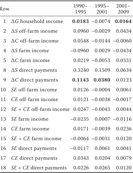
The subsequent section is devoted to the question if changes in the share or the concentration of the off-farm and farm income led to a change in the Gini coefficient of the total household income. Also the results for direct payments in general are presented. Table 2 shows a small but significant increase in the household income inequality from the pre-reform year 1990 to the post-reform year 1995 and between 2001 and 2009. In contrast, a slight but insignificant decrease of the income inequality can be observed between 1995 and 2001 (row 1 of Table 2).
The sum of the share and the concentration effect (row 12 and 15 respectively) shows that the off-farm income contributed to the income inequality in-creases between 1990 and 1995, while the decrease in the importance of the farm income alone would have reduced the overall income inequality (i.e. the negative share effect (row13) overcompensates the positive concentration effect (row14)). Between 1995 and 2001, the decrease in the concentration of the farm and off-farm income decreased the Gini coef-ficient of the total household income. In contrast, between 2001 and 2009 the off-farm income led to the income inequality increases because of its in-creasing importance for the household income (row 10 to 12), and the farm income increased the income inequality because of its increased concentration to farmers in the upper tail of the income distribution (row 13 to 15).
Table 2, furthermore, shows the effect of changes in the share and concentration of direct payments (which are part of the farm income) on the Gini coefficient of the total household income. It shows that direct payments by themselves would have increased the 6Direct payments continued to support incomes in all deciles, but the relative shares and concentrations across the
[image:7.595.65.289.350.641.2]deciles shifted in favour of higher-income farmers.
Table 2. Sources of change in total household income inequality
household income inequality over all time periods considered. However, the changes in the remaining part of the farm income (i.e. income from market-able goods) more than compensated the inequality increasing effects of direct payments between 1990 and 2001. This was not the case in the subsequent time period (2001–2009) where the sum of the share and the concentration effect of direct payments equals that of the farm income (row 18 and 15 respectively).
The effect of different direct payments on the household income inequality
The decomposition of the household income inequality by the single direct payment programmes
Figure 2 shows the shares of the different direct payment programmes in the total household income for the years 1990, 1995, 2001 and 2009. It shows
that a number of different support programmes were developed over time. Note that all abbreviations for the direct payment programmes are explained below Figure 2. In the pre-reform period, the roughage animal payments for farmers in the hill and mountain regions (RAUhill) and the arable payments (Arable) were the most important support programmes at farm-level. However, market prices were high and single payments made up only between 6% and 2% of the total household income. With the agricultural policy reform in 1992, the market support was re-duced and the area-based payments (Area) became the most important direct payment programme, making up about 16% of the total household income in 1995. In addition, the payments for the ecological compensation area (Eco), the extensive crop produc-tion (Extenso) and for the integrated production (the latter is included in the category Rest in Figure 2) were introduced for which farmers could voluntarily apply (e.g. Finger 2010). However, these payments made up only 11% of the total household income,
1990 1995 2001 2009 Rest
Ecoqual Regout AFSS Extenso Eco Arable Areahill RAUhill RAU Area Hhp
%
on hous
ehol
d i
n
c
o
m
e
02
0
4
0
6
0
8
[image:8.595.125.432.354.624.2]0
Figure 2. The share of different direct payments in the total household income
compared to all other direct payment programmes that contribute with 45%.
With the second policy reform step in 1999, the household payments and the support for the integrated production were abandoned but the production re-quirements of the integrated production programme became obligatory to receive the general direct pay-ments (see also section 2). Furthermore, the animal unit based payments without geographical restric-tions (RAU) were introduced as well as two animal welfare programmes (Regout, AFSS) and a programme that aims at supporting the ecological quality of the farm land (Ecoqual). The importance of the general direct payments for the household income increased to 59% in 2001 (with the area-based payments being the most important with 38% of the total household income) while the ecological direct payments still contribute with 11% to the total household income (see Figure 2).
Since the second reform step in 1999, only small changes were made to the direct payments system. The area-based direct payments were slightly de-creased which resulted in a decreasing share of these payments in the total household income. In contrast,
the animal unit based payments were made available to milking cows (which was not the case before) and the eco-quality payments were increased. In 2009, the general direct payments made up about 64% and the ecological direct payments 15% of the household income (see Figure 2).
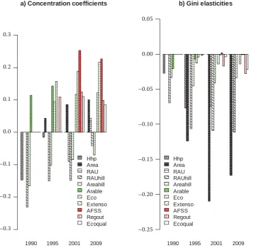
Figure 3a shows the concentration coefficients and the Gini elasticities for different direct pay-ments for the four considered years. It shows that the farm household payments (Hhp), the payments given to farmers producing under adverse production conditions (Areahill, RAUhill) support mainly the low-income farmers (i.e. have negative Gini concen-tration coefficients). Hence, these payments seem to be well targeted, as especially those farmers are supported by these programmes that are not able to generate an appropriate income from marketable goods because of the adverse production conditions they face.
In contrast, all other direct payments support mainly the farmers with the higher income levels (i.e. have positive Gini concentration coefficients). This is especially true for the animal welfare pro-gramme AFSS, which requires the farmer to construct
1990 1995 2001 2009 Hhp Area RAU RAUhill Areahill Arable Eco Extenso AFSS Regout Ecoqual
a) Concentration coefficients
-0
.3
-0
.2
-0
.1
0
.0
0
.1
0
.2
0
.3
1990 1995 2001 2009 Hhp
Area RAU RAUhill Areahill Arable Eco Extenso AFSS Regout Ecoqual
b) Gini elasticities
-0
.2
5
-0
.2
0
-0
.1
5
-0
.1
0
-0
.0
5
0
.0
0
0
.0
[image:9.595.110.469.402.751.2]5
Figure 3. Concentration coefficients and the Gini elasticities of different direct payment programmes
0.3
0.2
0.1
0.0
–0.1
–0.2
–0.3
0.05
0.00
–0.05
–0.10
–0.15
–0.20
a particularly animal-friendly stabling system. The result suggests that those farmers that generate the highest incomes are also those who are able to in-vest in the new stabling systems that are required to receive the additional direct payments. However, the concentration coefficients for each of the direct payment programmes are in general much lower than the Gini coefficient of the total household income. This implies that every of the direct payments help to decrease the household income inequality. This is also shown by the results of the Gini elasticities, depicted in Figure 3b. For instance, the increase of the area-based payments (Area) of 1% would have
decreased the household income inequality by 0.17% in 2009. The increase in the animal unit based pay-ments by 1% would have decreased the overall Gini coefficient by 0.11%. In contrast, the increase of support for the welfare and ecological programmes would hardly affect the income distribution of the household income.
The effect of different direct payments on changes in the household income inequality
Table 3 shows how the changes in the share and concentration of the different direct payments
pro-Table 3. The e ffect of different direct payments on changes in household income inequality
Line 1990–1995 1995–2001 2001–2009 Line 1990–1995 1995–2001 2001–2009 1 ΔG farm income 0.0183 –0.0074 0.0164
Farm household payments (CHF/farm household) Animal-friendly stabling systems (CHF/AUb)
2 ΔS 0.0520 – – 20 ΔS – – 0.0040
3 ΔC 0.1160 – – 21 ΔC – – –0.0554
4 SE + CE 0.0013 – – 22 SE + CE – – 0.0002
Arable payments (CHF/ha crop land) Livestock with regular outdoor exercise (CHF/AUb)
5 ΔS –0.0207 – – 23 ΔS – 0.0331 0.0053
6 ΔC 0.0218 – – 24 ΔC – 0.0183 –0.0476
7 SE + CE –0.0029 – – 25 SE + CE – 0.0047 –0.0013
Area-based payments(CHF/ha) Ecological compensation area (CHF/ha)
8 ΔS – 0.2012 –0.0536 26 ΔS – 0.0100 –0.0024
9 ΔC – 0.0475 0.0057 27 ΔC – 0.0212 0.0006
10 SE + CE – 0.0274 –0.0039 28 SE + CE – 0.0017 0.0003
Area-based payments; hill (CHF/ha) Extensive crop production (CHF/ha)
11 ΔS 0.0095 –0.0028 –0.0041 29 ΔS – –0.0031 –0.0018
12 ΔC 0.0349 0.0231 0.0057 30 ΔC – 0.0304 0.0186
13 SE + CE –0.0002 0.0010 0.0005 31 SE + CE – –0.0003 –0.0003
Animal unit based payments (CHF/RAU*) Ecoquality (CHF/ha)
14 ΔS – – 0.0628 32 ΔS – – 0.0236
15 ΔC – – 0.1179 33 ΔC – – –0.0641
16 SE + CE – – 0.0092 34 SE + CE – – 0.0010
Animal unit based payments; hill (CHF/RAUa)
17 ΔS 0.0257 –0.0041 0.0202
18 ΔC 0.0538 0.0030 0.0932
19 SE + CE –0.0017 0.0008 0.0049
[image:10.595.68.527.272.705.2]grammes affected the changes in the Gini coefficient of the total household income7. Between 1990 and
1995, the changes in the farm household payments (rows 2–4 in Table 3), which were mainly caused by the increase in the concentration effect, contributed to the income inequality increases. In contrast, the decreasing share of the arable payments (rows 5–6) would have led to a reduction in the Gini coefficient over time. Even though the share and the concentra-tion of the area- and animal-unit based payments for the hill and mountain regions increased (rows 11–13 and 17–19), these payments strongly supported farmers with low household incomes and therefore they would have reduced the overall Gini coefficient. Between 1995 and 2001, most direct payment pro-grammes positively contributed to the changes in the household income inequality. Significant increases in the share of the different payments on the household income can be observed for most of the programmes, while the changes in the concentration (i.e. Pseudo-Ginis) were only significant in the case of the area-based payments. In total, the increasing shares (i.e. share effect) of the here considered programmes would have increased the Gini coefficient of the total household income (which did not change significantly over this time period due to the shifts in the concentra-tion and the shares of the other income components). Between 2001 and 2009, the changes in the area-based payments (rows 8–10), the ecological compensation area payments (rows 26–28) and the payments for the extensive crop production (rows 29–31) would have reduced the household income inequality. For these programmes, the negative share effect was stronger than the positive concentration effect. In contrast, all other direct payments programmes increased the household income inequality. For instance, in the case of the eco-quality payments (rows 32–34), the increasing share more than compensated the decrease in the concentration. In contrast, in the case of the animal unit based payments (in the valley as well as hill regions), the concentration effect was much stronger. The disaggregated analysis shows that most of the direct payments affect the income inequality because of the changes in their share in household income. However, in the case of the animal-unit based pay-ments, also the increase in the concentration to farm-ers with higher incomes leads to the overall income inequality increases.
SUMMARY AND DISCUSSION
Our analysis showed that the total household income inequality in Swiss agriculture only slightly increased between 1990 and 2009, but a strong increase in the farm income inequality could be observed in this period. Hence, the strong reliance on direct pay-ments which Swiss farms have developed over the last 20 years has not led to a significant change in the sectoral inequality altogether. However, the change from the market support to the decoupled direct payments increased the number of farmers earning negative market incomes which led to an increase in the farm income inequality. The difference between the household income and the farm income inequality furthermore shows that the off-farm income plays an important role in balancing the income distribution among farmers.
Compared to other countries, however, the farm income within the Swiss farm population is still rather equally distributed with the Gini coefficients ranging between 0.27 and 0.38. In contrast, the Gini coeffi-cients of between 0.63 and 0.55 were found for Ireland (Keeney 2000), and the Gini coefficient of 0.54 was found for Germany (von Witzke and Noleppa 2007). This result can be explained by the homogenous struc-ture of Swiss agriculstruc-ture that is based on small family farms with a similar capital intensity (cp. Finger and El Benni 2011). Even though the structural change took place within the last two decades, no large and highly efficient farm operations were developed. The average farm size is about 17 hectare and 97% of all farms have 50 ha or less (FOA 2010).
Over the last two decades, the goals and measures of Swiss agricultural policy changed. These changes are reflected in the effects of direct payments on the household income inequality (i.e. the results of the Gini decomposition). In the pre-reform period, the main goal of direct payments was to support farm-ers that were disadvantaged by advfarm-erse production conditions and did not earn an appropriate income, even though the market support led to very high price levels. Hence, direct payments were not equally distributed and were given to farmers with low in-comes. With the agricultural policy reform in 1992, market support was reduced and direct payments aimed at compensating all farmers for income losses they face due to the price decreases. As a result of
the reform, direct payments became more equally distributed across farmers, but they were since also more concentrated on the farmers in the upper tail of the income distribution (see also Mann 2006). Hence, the new agricultural policy, which was based on the area payments, conserved the distributional effects of the former (market support oriented) policy at least to a certain extent. As in the case with the market support, also the support through direct payments advantaged the high income farmers (i.e. input fac-tors such as land enable farmers to produce more output but they also determine the amount of direct payments the farmers receive). However, even if the high-income farmers receive more direct payments than the low-income farmers, the direct farm-level support has still an equalizing effect on the income distribution (see also Keeney 2000; Mishra et al. 2009). Hence, the equalizing effect of direct payments can be attributed to the fact that the incomes in the lower tail of the income distribution can be maintained at a certain level.
Regarding the causes of the change of the household income inequality between the pre-reform year 1990 and the post-reform year 1995, our analysis shows that the off-farm income was the main contributor to the inequality increases. In contrast, changes in the share and the concentration of farm income hardly affected the Gini coefficient of the total household income over this time period. This implies that direct payments could compensate farmers for the foregone market profits without affecting the income distribution. In contrast, the household income inequality increases between 2001 and 2009 can mainly be attributed to the changes in farm income. Hence, even if the direct payments make up a considerable amount of the household income, they cannot avoid the income inequality increases. In addition, the income from direct payments exceeds the farm income which shows that direct payments are used to cover production costs and cannot compensate for the income losses anymore. This suggests that the income from farmers in the lower tail of the income distribution further decreases which opens the income gap across the farm population. Hence, a structural change is needed to enable farmers earning an appropriate income from farming. Furthermore, direct payments cannot be used to decrease the income inequality but the off-farm income might be a better strategy to balance the income between farmers.
The decomposition of the Gini coefficient by the single direct payment programmes reveals the inequal-ity reducing effect from each of the direct payment programmes considered. This is especially true for the general direct payments that make up a high share
in the household income. In contrast, the increase of income from the animal welfare payments and the ecological direct payments would hardly affect the distribution of farm income.
The disaggregated analysis over time shows that the changes in the share (i.e. the share of a specific direct payment programme in the household income) are the primary reason why a single direct payment programme contributes to the household income inequality. However, this seems to be rather the case for the area-based payments than for the animal-unit based payments, for which also the changes in the concentration contributed to the income inequality changes in the past. In general, the contribution of the general direct payments to the inequality changes is higher than the contribution of the ecological direct payments. This, however, is the result of the low importance of these payments for the household income and may change if the agricultural policy opts to increase the support for the environmental friendly production.
REFERENCES
Allanson P. (2005): The Impact of Farm Income Support on Absolute Inequality. Paper for the 94th EAAE Seminar, 9–10 April 2005, Ashford, UK.
Boisvert R.N., Ranney C. (1990): Accounting for the im-portance of non-farm income on farm family income inequality in New York. Northeastern Journal of Agri-cultural Economics, 19: 1–11.
Chen C.-N., Tsaur T., Rhai T.S. (1982): The Gini coef-ficient and negative income. Oxford Economic Papers, 36: 473–476.
Curry N., Stucki E. (1997): Swiss agricultural policy and the environment: an example for the rest of Europe to follow? Journal of Environmental Planning and Manage-ment, 40: 465–482.
DiCiccio T.J., Efron B. (1996): Bootstrap confidence inter-vals. Statistical Science, 11: 189–212.
El Benni N., Lehmann B. (2010): Swiss agricultural policy reform: landscape changes in consequence of national agricultural policy and international competition pres-sure. In: Primdahl J., Swaffield S. (eds.): Globalisation and Agricultural Landscapes – Change Patterns and Policy trends in Developed Countries. Cambridge Uni-versity Press, Cambridge, pp. 73–94.
Engler M. (2010): Redistribution in Switzerland: Social Cohesion or Simple Smoothing of Lifetime Incomes? Discussion Paper No. 2010-02, Department of Econom-ics, University of St. Gallen.
Forschungsanstalt für Agrarwirtschaft und Landtechnik (FAT), Tänikon.
Fei J.C.H., Ranis G., Kuo S.W.Y. (1978): Growth and the family distribution of income by factor components. The Quarterly Journal of Economics, 92: 17–53.
Finger R. (2010): Evidence of slowing yield growth – the example of Swiss cereal yields. Food Policy, 35: 175–182. Finger R., El Benni N. (2011): Spatial analysis of income
inequality in agriculture. Economics Bulletin, 31: 2138– 2150.
Flückiger Y., Silber J. (1995): Income inequality decomposi-tion by income source and the breakdown of inequality differences between two population subgroups. Swiss Journal of Economics and Statistics, 131: 599–615. FOA (2010): Agricultural report 2010. Swiss Federal Office
of Agriculture, Bern, Switzerland.
Gerfin M. (1994): Income distribution, income inequality and life cycle effects – a nonparametric analysis for Switzerland. Swiss Journal of Economics and Statistics, 130: 509–522.
Hill B. (1999): Farm household incomes: perceptions and statistics. Journal of Rural Studies, 15: 345–358. Keeney M. (2000): The distributional impact of direct
pay-ments on Irish farm incomes. Journal of Agricultural Economics, 51: 252–263.
Lerman R.I., Yitzhaki S. (1985): Income inequality effects by income source: a new approach and applications to the United States. The Review of Economics and Sta-tistics, 67: 151–156.
Mann S. (2003): Doing it the Swiss way. EuroChoices, 2: 32–35.
Mann S. (2005): Implicit social policy in agriculture. Social Policy and Society, 4: 271–281.
Mann S. (2006): Direktzahlungen aus sozialpolitischer Perspektive am Beispiel der Schweizer Landwirtschaft. Zeitschrift für Agrarpolitik und Landwirtschaft, 84: 116–127.
Mishra A., El-Osta H., Gillespie J.M. (2009): Effect of ag-ricultural policy on regional income inequality among farm households. Journal of Policy Modeling, 31: 325– 340.
Moreddu C. (2011): Distribution of Support and Income in Agriculture. OECD Food, Agriculture and Fisheries Working Papers, No. 46, OECD Publishing, Paris. OECD (1998): Agriculture in a Changing World: Which
Policies for Tomorrow? Organisation for Economic Co-operation and Development (OECD), Paris.
Podder N. (1995): On the relationship between the Gini coefficient and income elasticity. Sankya: The Indian Journal of Statistics, 57 (Series B, Part 3): 428–432. Podder N., Chatterjee S. (2002): Sharing the national cake
in post reform New Zealand; income inequality trends in terms of income sources. Journal of Public Econom-ics, 86: 1–27.
Pyatt G., Chau-nan C., Fei J. (1980): The distribution of income by factor components. The Quarterly Journal of Economics, 95: 451–473.
R Development Core Team (2011): R: A language and environment for statistical computing. R Foundation for Statistical Computing, Vienna, Austria. Available at www.R-project.org
Schmid E., Hofreither M.F., Sinabell F. (2006): Impacts of CAP Instruments on the Distribution of Farm Incomes – Results for Austria. Discussion paper DP-13-2006, Universität für Bodenkultur, Wien.
Schenker N., Gentleman J.F. (2001): On judging the signifi-cance of differences by examining the overlap between confidence intervals. The American Statistician, 55: 182–186.
Stuart A. (1954): The correlation between variate-values and ranks in samples from a continuous distribution. British Journal of Statistical Psychology, 7: 37–44. Van de Ven J. (2001): Distributional Limits and the Gini
Coefficient. Research Paper Number 776, January 2001, Department of Economics, University of Melbourne, Melbourne.
von Witzke H., Noleppa S. (2007): Agricultural and Trade Policy Reform and Inequality: The Distributive Effects of Direct Payments to German Farmers under the EU’s New Common Agricultural Policy. Working Paper Series No. 79/2007, Institute for Agricultural Economics and Social Sciences, Humboldt-University of Berlin, Berlin. Zürcher B.A. (2004): Income inequality and mobility: a nonparametric decomposition analysis by age for Swit-zerland in the 80s and 90s. Swiss Journal of Economics and Statistics, 140: 265–292.
Arrived on 21th December 2011
Note: Current affiliation co-author Robert Finger: Agricultural Economics and Rural Policy Group, Wageningen University, The Netherlands
Contact address:
Nadja El Benni, Swiss Federal Institute of Technology Zurich (ETH Zürich), Sonneggstrasse 33, CH-8092 Zurich, Switzerland