Comparing the Performance of Feature Representations for the Categorization of the Easy to Read Variety vs Standard Language

(1)

Comparing the Performance of Feature Representations

for the Categorization of the Easy-to-Read Variety vs Standard Language

Marina Santini

RISE Research Institutes of Sweden (Division ICT - RISE SICS East)

Stockholm, Sweden [email protected]

Benjamin Danielsson

Link¨oping University (IDA)

Link¨oping, Sweden [email protected]

Arne J¨onsson

RISE Research Institutes of Sweden & Link¨oping University (IDA)

Link¨oping, Sweden [email protected]

Abstract

We explore the effectiveness of four fea-ture representations – bag-of-words, word embeddings, principal components and autoencoders – for the binary categoriza-tion of the easy-to-read variety vs standard language. “Standard language” refers to the ordinary language variety used by a population as a whole or by a community, while the “easy-to-read” variety is a sim-pler (or a simplified) version of the stan-dard language. We test the efficiency of these feature representations on three cor-pora, which differ in size, class balance, unit of analysis, language and topic. We rely on supervised and unsupervised ma-chine learning algorithms. Results show that bag-of-words is a robust and straight-forward feature representation for this task and performs well in many experimen-tal settings. Its performance is equiva-lent or equal to the performance achieved with principal components and autoen-corders, whose preprocessing is however more time-consuming. Word embeddings are less accurate than the other feature rep-resentations for this classification task.

1 Introduction

Broadly speaking, a language variety is any spe-cific form of language variation, such as standard language, dialects, registers or jargons. In this pa-per, we focus on two language varieties, namely the standard language variety and the easy-to-read variety. In this context, “standard language” refers to the official and ordinary language variety used by a population as a whole, or to a variety that is normally employed within a community. For ex-ample, “Standard English” is the form of the En-glish language widely accepted as the usual cor-rect form, while within the medical community it

is the specialized medical jargon that is considered to be standard language. In contrast, the easy-to-read variety is a simpler version of a standard lan-guage. The need of an easy-to-read variety stems from the difficulties that certain groups of people experience with standard language, such as people with dyslexia and other learning disabilities, the elderly, children, non-native speakers and so on. In order to meet the needs of a simpler language that makes information easy to read and under-stand for all, European Standards have been estab-lished1, and an important initiative like Wikipedia has created a special edition called Simple En-glish Wikipedia2. These are not isolated phenom-ena. For instance, in Sweden public authorities (sv:myndigheter) provide an easy-to-read version (a.k.a. simple Swedish or sv: l¨attl¨ast) of their writ-ten documentation.

Both in the case of the Simple English Wikipedia and in the case of Swedish public au-thorities, the simplified documents are manually written. Since the manual production of simplified texts is time-consuming, the task called Text Sim-plification (TS) is very active in Natural Language Processing (NLP) in the attempt to streamline this type of text production. TS is a fast-growing re-search area that can bring about practical benefits, e.g. the automatic generation of simplified texts. There is, however, a TS subtask that is still un-derexplored: the categorization of the easy-to-read variety vs standard language. The findings pre-sented in this paper contribute to start filling this gap. The automatic separation of standard texts from easy-to-read texts could be particularly use-ful for other TS subtasks, such as the bootstrap-ping of monolingual corpora from the web or the

1_{https://easy-to-read.eu/wp-content/}

uploads/2014/12/EN_Information_for_all. pdf

2_{https://simple.wikipedia.org/wiki/}

(2)

extraction of simplified terminology. Other ar-eas that could benefit from it include informa-tion retrieval (e.g. for the retrieval of easy-to-read or patient-friendly medical information) and deep learning-based dialogue systems (e.g. customized chatbots for expert users or naive users).

The research question we would like to an-swer is: which is the most suitable feature rep-resentation for this categorization task? In or-der to answer this question, we compare four dif-ferent feature representations that can potentially make sense of the lexical makeup that differenti-ates easy-to-read from standard language, namely bag-of-words (BoWs), word embeddings, princi-pal components and autoencoders. It goes without saying that these four feature representations are just a few of the many possible feature representa-tions for this kind of task. We start our long-term exploration with these four feature representations because they are straightforward and easy to ex-tract automatically from any corpora. We test the efficiency of the four feature representations with three types of machine learning algorithms: tra-ditional supervised machine learning, deep learn-ing and clusterlearn-ing3. The experiments are based on three corpora belonging to different domains. From these corpora, we extracted three datasets of different sizes, different class balance, different units of analysis (sentence vs document), different languages (Swedish and English).

The ultimate goal of the experiments presented in this paper is to propose a first empirical baseline for the categorization of the easy-to-read variety vs standard language.

2 Previous Work

As mentioned above, the automatic separation of standard language from the easy-to-read variety is underinvestigated, but it could be useful for sev-eral TS subtasks, such as the bootstrapping (Ba-roni and Bernardini, 2004) of monolingual paral-lel corpora (Caseli et al., 2009), of monolingual comparable corpora (Barzilay and Elhadad, 2003) or the exploitation of regular corpora (Glavaˇs and ˇStajner, 2015). Extensive work exists in TS (Sag-gion, 2017). The most advanced work focuses on the implementation of neural text simplifica-tion systems that are able to simultaneously per-form lexical simplification and content reduction

3_{The umbrella term ‘categorization’ is used to cover these}

three machine learning approaches.

(Nisioi et al., 2017).

In this paper, however, we do not focus on the creation of TS systems, but rather on the sheer downstream categorization task of separating stan-dard language from the easy-to-read variety. To our knowledge, limited research exists in this area, which mostly focuses on the discrimination be-tween the specialized language used by domain experts and the language used by non-experts (a.k.a. laypeople or the lay). This type of distinc-tion is required in some domains (e.g. medical and legal domains), where the specialized jargon hin-ders the unhin-derstanding of “ordinary” people, i.e. people without specialized education, who strug-gle to get a grip on professional sublanguages. In the experiments reported in Santini et al. (2019), it is shown that it is possible to successfully dis-criminate between medical web texts written for experts and for laypeople in Swedish. Results are encouraging and we use one of their datasets in the experiments presented here.

Other corpora are available that can be used for the automatic categorization of the easy-to-read variety vs standard language. For instance, the Simple English Wikipedia corpus4 (Kauchak, 2013), and the DigInclude corpus5 in Swedish (Rennes and J¨onsson, 2016). However, neither Simple English Wikipedia nor DigInclude have ever been used for this text categorization task. We use them in this context for the first time.

3 Corpora and Datasets

In our experiments, we use three corpora, two in Swedish and one in English. More precisely, we rely on 1) a subset of the eCare corpus (San-tini et al., 2019) in Swedish; 2) a subset of the DigInclude corpus (Rennes and J¨onsson, 2016) in Swedish and 3) a subset of the Simple English Wikipedia corpus (Kauchak, 2013) in English.

The eCare corpus is a domain-specific web cor-pus. The domain of interest is the medical field of chronic diseases. From the current version of the corpus we re-use a labelled subset. The eCare sub-set contains 462 webpages without boilerplates. The webpages have been labelled as ‘lay’ or ‘spe-cialized’ by a lay native speaker. Lay sublanguage is an easy-to-read version of the standard lan-guage(the medical jargon) used by healthcare

pro-4

http://www.cs.pomona.edu/˜dkauchak/ simplification/

5

(3)

fessionals. The 462 webpages of the eCare dataset (amounting to 424,278 words) have been labelled in the following way: 388 specialized webpages (66%) and 154 lay webpages (33%). The dataset is unbalanced. The unit of analysis that we use in these experiments is thedocument.

The DigInclude corpus is a collection of easy-to-read sentences aligned to standard language sentences. The corpus has been crawled from a number of Swedish authorities’ websites. The DigInclude datasets contains 17,502 sentences, 3,827 simple sentences (22%) and 13,675 standard sentences (78%), amounting to 233,094 words. The dataset is heavily unbalanced. The unit of analysis is thesentence.

The Simple English Wikipedia (SEW) cor-pus was generated by aligning Simple English Wikipedia and standard English Wikipedia. Two different versions of the corpus exist (V1 and V2). V2 has been packaged in sentences and in docu-ments. We used the subset of V2 divided into tences. The SEW dataset contains 325,245 sen-tences, 159,713 easy-to-read sentences (49.1%) and 165,532 standard sentences (50.9%), amount-ing to 7,191,133 words. The dataset is fairly bal-anced. The unit of analysis is thesentence.

4 Features Representations and Filters

At the landing page of Simple English Wikipedia, it is stated: “We use Simple English words and grammar here.” Essentially, this statement implies that the use of basic vocabulary and simple gram-mar makes a text easier to read. In these experi-ments we focus on the effectiveness of feature rep-resentations based onlexical itemsand leave the exploration of grammar-based tags for the future.

In this section, we describe the four feature representations, as well as the filters that have been applied to create them. These filters and the methods described in Section 5 are included in the Weka Data Mining workbench (Witten et al., 2016)6. All the experiments performed with the Weka workbench can be replicated in any other workbench, or programmatically in any program-ming language. We use Weka here for the sake of fast reproducibility, since Weka is easy to use also for those who are not familiar with the practicali-ties of machine learning. Additionally, it is open source, flexible and well-documented.

6_{Open source software freely available at} _https://

www.cs.waikato.ac.nz/ml/weka/

In the experiments below several filters have been stacked together via the Multifilter metafil-ter, which gives the opportunity to apply several filtering schemes sequentially to the same dataset.

BoWs. BoWs is a representation of text that de-scribes the occurrence of single words within a document. It involves two things: a vocabulary of known words and a weighing scheme to mea-sure the presence of known words. It is called a “bag” of words, because any information about the order or structure of words in the document is dis-carded. The model is only concerned with whether known words occur in the document, not where in the document, or with which other words they co-occur. The advantage of BoWs is simplicity. BoWs models are simple to understand and im-plement and offer a lot of flexibility for customiza-tion. Preprocessing can include different levels of refinement, from stopword removal to stemming or lemmatization, and a wide range of weighing schemes. Usually, lexical items in the form of BoWs represent the topic(s) of a text and are nor-mally used for topical text classification. Several related topics make up a domain, i.e. a subject field like Fashion or Medicine. Here we use BoWs for a different purpose, which is to detect the dif-ferent level of lexical sophistication that exists between the easy-to-read variety and standard lan-guage. Intuitively, easy-to-read texts have a much plainer and poorer vocabulary than texts written in standard language. Therationaleof using BoWs in this context is then to capture the lexical diver-sification that characterizes easy-to-read and stan-dard language texts.

Starting from datasets in string format, we ap-plied StringToWordVector, which is an unsuper-vised filter that converts string attributes into a set of attributes representing frequencies of word oc-currence. For all the corpora, we selected the TF and IDF weighing schemes, normalization to low-ercase and normalization to the length of the doc-uments. Lemmatization, stemming and stopword removal were not applied. The number of words that were kept varies according to the size of cor-pus. The complete settings of this and all the other filters described below are fully documented in the companion website.

(4)

effective in many tasks (e.g. sentiment analysis, text classification, etc.). The advantageof word embeddings lies in their capability to capture the context of a word in a document, as well as se-mantic and syntactic similarity. The basic idea be-hind word embeddings is to “embed” a word vec-tor space into another. The big intuition is that this mapping could bring to light something new about the data that was unknown before. More specifi-cally, word embeddings learn both the meanings of the words and the relationships between words because they capture the implicit relations be-tween words by determining how often a word ap-pears with other words in the training text. The

rationale of using word embeddings in this con-text is to account for both semantic and syntactic representations, traits that can be beneficial for the categorization of language varieties.

Word embeddings can be native or pretrained. Here we use the pretrained Polyglot Embed-dings (Al-Rfou et al., 2013) for Swedish (polyglot-sv) and for English (polyglot-en).

Principal Components. Principal Component Analysis (PCA) involves the orthogonal transfor-mation of possibly correlated variables into a set of values of linearly uncorrelated variables called principal components. This transformation is de-fined in such a way that the first principal com-ponent explains the largest possible variance, and each succeeding component in turn explains the highest variance possible under the constraint that it is orthogonal to the preceding components. The

advantageof PCA is to reduce the number of re-dundant features, which might be common but dis-turbing when using a BoWs approach, thus possi-bly improving text classification results. The ra-tionale of using PCA components in this context is to ascertain whether feature reduction is benefi-cial for the categorization of language varieties.

To perform PCA and the transformation of the data, we wrapped PrincipalComponentsfilter on the top of the StringToWordVector filter, via the Multifilter metafilter. The PrincipalComponents

filter is an unsupervised filter that chooses enough principal components (a.k.a eigenvectors) to ac-count for 95% of the variance in the original data.

Autoencoders. Similar to PCA, the basic idea behind autoencoders is dimensionality reduction. However, autoencoders are much more flexible than PCA since they can represent both linear and

non-linear transformation, while PCA can only perform linear transformation. Additionally, au-toencoders can be layered to form deep learning networks. They can also be more efficient in terms of model parameters since a single autoencoder can learn several layers rather than learning one huge transformation as with PCA. Theadvantage

of using autoencoders in this context is to trans-form inputs into outputs with the minimum possi-ble error (Hinton and Salakhutdinov, 2006). The

rationaleof their use here is to determine whether they provide a representation with enriched prop-erties that is neater than other reduced representa-tions.

In these experiments, autoencoders are gener-ated using theMLPAutoencoder filter stacked on the top of the StringToWordVector filter, via the Multifilter metafilter. This MLPAutoencoder fil-ter gives the possibility of creating contractive au-toencoders, which are much more efficient than standard autoencoders (Rifai et al., 2011).

5 Methods, Baselines and Evaluation

In this section, we describe the categorization schemes, the baselines and the evaluation metrics used for comparison.

Methods. We use three different learning meth-ods, namely an implementation of SVM, an imple-mentation of multilayer perceptron (MLP) and an implementation of K-Means for clustering. The rationale behind these choices is to compare the behaviour of the four feature representations de-scribed above with learning schemes that have a different inductive biases, and to assess the differ-ence (if any) between the performance achieved with labelled data (supervised algorithms) and un-labelled data (clustering). We calculate a random baseline with the ZeroR classifier. All the catego-rization schemes are described below.

ZeroR: baseline classifier. The ZeroR is based on the Zero Rule algorithm and predicts the class value that has the most observations in the train-ing dataset. It is more reliable than a completely random baseline.

(5)

vector classifier (Joachims, 1998).

Since two corpora are highly unbalanced, we also combined SMO with filters that can cor-rect class unbalance. More specifically, we re-lied on ClassBalancer, which reweights the in-stances in the data so that each class has the same total weight; Resample, which produces a random subsample of a dataset using either sam-pling with replacement or without replacement;

SMOTE, which resamples a dataset by applying

the Synthetic Minority Oversampling TEchnique (SMOTE); andSpreadSubsample, which produces a random subsample of a dataset. All the models built with SMO are based on Weka’s standard pa-rameters.

Multilayer Perceptron: Deep Learning. Weka

provides several implementations of MLP. We re-lied on the WekaDeeplearning4j package that is described in Lang et al. (2019). The main clas-sifier in this package is named DI4jMlpClasclas-sifier and is a wrapper for the DeepLearning4j library7 to train a multilayer perceptron. While fea-tures like BoWs, principal components and au-toencoders can be fed to any classifiers within the Weka workbench (if they are wrapped in fil-ters), word embeddings can be handled only by the DI4jMlpClassifier (this explains N/A in Ta-ble 2). We used the standard configuration of the DI4jMlpClassifier (which includes only one output layer) for BoWs, principal components and autoencoders. Conversely, the configura-tion used with word embeddings was cutomized in the following way: word embeddings were passed through four layers (two convulational lay-ers, a GlobalPoolingLayer and a OutputLayer); the number of epochs was set to 100; the in-stance iterator was set on CnnTextEmbeddingIn-stanceIterator; we used the polyglot embeddings for Swedish and English, as mentioned above.

K-Means: Clustering. We compare the

perfor-mance of the supervised classification with clus-tering (fully unsupervised categorization). We use the traditional K-Means algorithm (Arthur and Vassilvitskii, 2007) that in Weka is called Sim-pleKMeans. Since we know the number of classes in advance (i.e. two classes), we evaluate the qual-ity of the clusters against existing classes using the option Classes to cluster evaluation, which first ignores the class attribute and generates the

clus-7_{https://deeplearning.cms.waikato.ac.}

nz/

ters, then during the test phase assigns classes to the clusters, based on the majority value of the class attribute within each cluster.

Evaluation metrics. We compare the perfor-mances on the Weighted Averaged F-Measure (AvgF), which is the sum of all the classes’ F-measures, each weighted according to the number of instances with that particular class label.

In order to reliably assess the performance based on AvgF, we also usek-statisticand theROC area value. K-statistic indicates the agreement of prediction with true class; when the value is 0 the agreement is random. The quality of a classifier can also be assessed with the help of the ROC area value which indicates the area under the ROC curve (AUC). It is used to measure how well a classifier performs. The ROC area value lies be-tween about 0.500 to 1, where 0.500 (and below) denotes a bad classifier and 1 denotes an excellent classifier.

ZeroR Baselines. Table 1 shows a breakdown of the baselines returned by the ZeroR classifier on the three corpora. These baselines imply that the k-statistic is 0 and the ROC area value is below or equal to 0.500.

6 Results and Discussion

The main results are summarized in Table 2 and Table 3. As shown in in Table 2, by and large both SMO and the DI4jMlpClassifier have equivalent or identical performance on all datasets in combi-nation with BoWs and principal components (we observe however that the DI4jMlpClassifier is def-initely slower than SMO). Word embeddings have a slightly lower performance than BoWs and prin-cipal components on the eCare and SEW subsets. Autoencoders perform well (0.82) in combination with SMO on the eCare subset, less so (0.77) when running with the DI4jMlpClassifier. The perfor-mance of clustering with BoWs on eCare gives an encouraging 0.59 (6 points above the ZeroR base-line of 0.53), while the performance with principal components and autoencoders is below the ZeroR baselines. In short, BoWs, which is the simplest and the most straightforward feature representa-tion in this set of experiments, has a performance that is equivalent or identical to other more com-plex feature representations.

(6)

[image:6.595.97.504.85.176.2]

Table 1: ZeroR baselines, breakdown

Class k Acc(%) Err(%) P R F ROC

eCare Subset (462 webpages)

lay (154 webpages)

0.00 66.66 33.33 0.00 0.00 0.00 0.490 specialized (308 webpages) 0.66 1.00 0.80 0.490

AvgF 0.53

DigInclude Subset (17,502 sentences)

simplified (3,827 sentences)

0.00 78.13 21.86 0.00 0.00 0.00 0.500 specialized (13,675 sentences) 0.78 1.00 0.87 0.500

AvgF 0.68

SEW Subset (325,235 sentences)

simplified (159,708 sentences)

0.00 50.89 49.10 0.00 0.00 0.00 0.500 specialized (165,527 sentences) 0.50 1.00 0.67 0.500

[image:6.595.111.484.208.348.2]

AvgF 0.34

Table 2: Summary table (AvgF): easy-to-read variety vs standard language

Dataset Features SMO DI4jMlp K-Means

eCare Subset

BoW Features 0.80 0.80 0.59

Word Embeddings N/A 0.75 N/A

Principal Components 0.80 0.81 0.44

Autoencoders 0.82 0.77 0.50

DigInclude Subset

BoW 0.72 0.72 0.29

SEW Subset

BoW 0.58 0.56 0.43

Table 3: Summary table (AvgF): unbalanced datasets (BoWs + class balancing filters applied to SMO)

Dataset NoFilter ClassBalancer Resample SpreadSample SMOTE

eCare Subset 0.80 0.81 0.81 0.80 0.81

DigInclude Subset 0.72 0.68 0.66 0.73 0.74

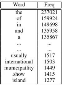
[image:6.595.131.233.561.698.2]

words that have been automatically selected by the StringToWordVector filter. Interestingly, since we did not apply stopword removal, the lexical items selected by the filter are mostly function words and common lexical items. An example is shown in Table 4.

Table 4: 5 top frequent words and 5 bottom fre-quent words in one of the SEW models

Word Freq

the 237021

of 159924

in 149698

and 135958

a 135867

... ...

usually 1517

international 1503 municipatlity 1449

show 1415

island 1277

At first glance, it might appear counter-intuitive that BoWs, which are very simple features that do not take syntax and word order into account, can perform well in this kind of task. However, we

surmize that this is the effect of the presence of stopwords. As stopwords have not been removed (see settings reported earlier), the classifiers do not learn ‘topics’ – since content words are pushed down in the rank of the frequency list – but rather the distribution of function words, that are instead top-ranked and represent “structural” lexical items that capture the syntax rather than the meaning of texts. Essentially, function words can be seen as a kind of subliminal syntactic features. What is more, in the corpora some words are domain-specific and difficult, while others are easy and common. Apparently, thisdifficult vs easy varia-tion in the vocabulary helps the classificavaria-tion task. The full list of the words extracted by the String-ToWordVectorFilter (utilized alone or as the basis of other filters) is available on the companion web-site.

(7)

feature representation that accounts for both syn-tactic information and lexical sophistication.

[image:7.595.306.520.218.658.2]

As for word embeddings, it seems that their full potential remains unleashed in this context. The-oretically, word embeddings would be an ideal feature representation for this task because they combine syntax and semantics and they could capture simplification devices both at lexical and morpho-syntactic level. However, this does not fully happen here. As a matter of fact, it has al-ready been noticed elsewhere that word embed-dings might have an unstable behaviour (Wend-landt et al., 2018) that needs to be further inves-tigated.

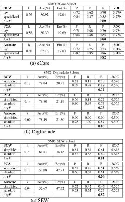
Table 5: SMO, breakdown

SMO: eCare Subset

BOW k Acc(%) Err(%) P R F ROC lay

0.56 80.92 19.04 0.72 0.68 0.70 0.779 specialized 0.84 0.87 0.85 0.779

AvgF 0.80

PCA k Acc(%) Err(%) P R F ROC lay

0.58 80.30 19.69 0.71 0.68 0.70 0.774 specialized 0.84 0.86 0.85 0.774

AvgF 0.80

Autoenc k Acc(%) Err(%) P R F ROC lay

0.60 82.16 17.83 0.72 0.75 0.73 0.804 specialized 0.87 0.85 0.86 0.804

AvgF 0.82

(a) eCare

SMO: DigInclude Subset

BOW k Acc(%) Err(%) P R F ROC simplified

0.13 79.04 20.95 0.61 0.11 0.18 0.546 standard 0.79 0.98 0.88 0.546

AvgF 0.72

PCA k Acc(%) Err(%) P R F ROC simplified

0.14 78.80 21.19 0.56 0.14 0.22 0.555 standard 0.80 0.97 0.77 0.555

AvgF 0.73

Autoenc k Acc(%) Err(%) P R F ROC simplified

0.00 78.49 21.50 0.00 0.00 0.00 0.500 standard 0.78 1.00 0.87 0.500

AvgF 0.68

(b) DigInclude

SMO: SEW Subset

0.23 61.81 38.18 0.61 0.61 0.61 0.618 standard 0.62 0.62 0.62 0.618

AvgF 0.61

0.13 57.08 42.91 0.57 0.45 0.51 0.569 standard 0.56 0.67 0.61 0.569

AvgF 0.56

0.04 52.67 47.32 0.52 0.42 0.46 0.525 standard 0.53 0.62 0.57 0.525

AvgF 0.52

(c) SEW

We observe that the classification results are promising on the eCare subset (see breakdown in Tables 5a, 6a and 7a). Arguably, a factor has contributed to achieve this performance: the unit of analysis. Certainly, classification at document level is easier because the classifier has more text to learn from. Surprisingly, the unbalance of the eCare dataset seems to be somehow mitigated by

the unit of analysis, since the classifiers are not bi-ased towards the majority class and k-statistic and ROC area values are quite robust (mostly above 0.500 and above 0.800 respectively). Additonally, the dataset is small, and this might also facilitate the learning. Clustering with BoWs is well above the ZeroR baseline, while with the other feature representations the performance is below the base-line thresholds.

Table 6: DI4jMlpClassifier, breakdown

DI4jMlpClassifier: eCare Subset

0.57 80.08 19.91 0.67 0.78 0.72 0.890 specialized 0.88 0.80 0.84 0.890

AvgF 0.80

Embed k Acc(%) Err(%) P R F ROC lay

0.45 75.79 24.20 0.63 0.65 0.64 0.807 specialized 0.82 0.81 0.81 0.807

AvgF 0.75

PCA k Acc(%) Err(%) P R F ROC lay

0.58 80.73 19.26 0.68 0.79 0.73 0.900 specialized 0.88 0.81 0.84 0.900

AvgF 0.81

Autoenc k Acc(%) Err(%) P R F ROC lay

0.52 77.07 22.92 0.61 0.84 0.71 0.872 specialized 0.90 0.73 0.81 0.872

AvgF 0.77

(a) eCare

DI4jMlpClassifier: DigInclude Subset

0.18 72.86 27.13 0.37 0.35 0.36 0.667 standard 0.82 0.83 0.82 0.667

AvgF 0.72

Embed k Acc(%) Err(%) P R F ROC simplified

0.10 77.24 22.75 0.41 0.13 0.20 0.587 standard 0.80 0.94 0.86 0.587

AvgF 0.72

0.16 72.94 27.05 0.36 0.31 0.33 0.650 standard 0.81 0.84 0.83 0.650

AvgF 0.72

0.00 78.49 21.50 0.00 0.00 0.00 0.500 standard 0.78 1.00 0.87 0.500

AvgF 0.68

(b) DigInclude

DI4jMlpClassifier: SEW Subset

0.13 56.50 43.49 0.55 0.57 0.56 0.594 standard 0.57 0.55 0.56 0.594

AvgF 0.56

Embed k Acc(%) Err(%) P R F ROC simplified

0.10 55.26 44.73 0.54 0.53 0.53 0.586 standard 0.55 0.57 0.56 0.586

AvgF 0.55

0.10 55.21 44.78 0.54 0.55 0.55 0.577 standard 0.56 0.54 0.55 0.577

AvgF 0.55

0.04 52.14 47.85 0.51 0.60 0.55 0.535 standard 0.53 0.44 0.48 0.535

AvgF 0.51

(c) SEW

[image:7.595.72.286.289.633.2]

(8)

combina-tion with SMO and the DI4jMlpClassifier are very close to random (see the value of k-statistic and the ROC area value). Although the AvgF values in the summary table (Table 2) seem to be decent for a binary classification problem, they are actually misleading, because the classifiers perform poorly on the minority class, as revealed by the low value of k-statistic and the ROC area value shown in the breakdown tables (Tables 5b and 6b). Classifi-cation with autoencoders is perfectly random (k-statistic 0.00 and ROC area value 0.500). Cluster-ing results are very poor with all feature represen-tations. Arguably, with this dataset the learning is hindered by two factors: the high class unbalance and the very short text that makes up a sentence. While in the case of the eCare subset, unbalance is compensated by the longer text of webpages, with DigInclude the sentence does not allow any gen-eralizable learning. Given these results, a differ-ent approach must be taken for datasets like Dig-Include. Solutions to address these problems in-clude changing the unit of analysis from sentences to documents (if possible) and/or applying a dif-ferent classification approach e.g. a cost-sensitive classifier of the kind used to predict rare events, e.g. Ali et al. (2015) or Krawczyk (2016). Algo-rithms used for fraud detection (Sundarkumar and Ravi, 2015) could also be useful.

The SEW corpus (see Tables 5c, 6c and 7c) is balanced and the unit of analysis is the sentence. The performance is promising because it is well above the ZeroR baseline (0.32). The best perfor-mance is with the combination of SMO and BoWs that reaches an AvgF of 0.58 with only a limited number of features. Word embeddings perform slightly worse than BoWs (but the running time is much longer). Clustering is definitely encour-aging and much above the baseline level with all features representations.

[image:8.595.348.514.76.428.2]

Since the eCare and DigInclude datasets are both unbalanced, we applied class balance correc-tors. Table 8 shows the breakdown of SMO on the eCare subset in combination with four balancing filters. The performance with filters is similar to the performance without filters. This is true also if we look at the performance (P, R, AvgF) of the minority class (the lay class). K-statistic is sta-ble (greater than 0.50) as are the ROC area values (greater than 0.700). Essentially, this means that this dataset, although unbalanced, does not need a class balancing filter. As pointed out earlier, we

Table 7: K-means, breakdown

K-means: eCare

BOW Acc(%) Err(%) P R F lay

60.82 39.18 0.48 0.75 0.56 specialized 0.81 0.53 0.64

AvgF 0.59

PCA Acc(%) Err(%) P R F lay

51.95 48.05 0.32 0.50 0.39 specialized 0.65 0.47 0.54

AvgF 0.44

Autoenc Acc(%) Err(%) P R F lay

54.55 45.45 0.37 0.57 0.45 specialized 0.71 0.53 0.61

AvgF 0.50

(a) eCare

Simple K-means: DigInclude

BOW Acc(%) Err(%) P R F simplified

75.78 24.22 0.21 0.93 0.35 standard 0.73 0.04 0.08

AvgF 0.29

PCA Acc(%) Err(%) P R F simplified

78.09 21.91 0.21 0 0 standard 0.78 0.99 0.87

AvgF 0.19

Autoenc Acc(%) Err(%) P R F simplified

54.54 45.46 0.22 0.62 0.33 standard 0.79 0.40 0.53

AvgF 0.37

(b) DigInclude

K-means: SEW

BOW Acc(%) Err(%) P R F simplified

50.27 49.73 0.46 0.17 0.25 standard 0.50 0.80 0.62

AvgF 0.43

PCA Acc(%) Err(%) P R F simplified

50.37 49.63 0.48 0.49 0.48 standard 0.50 0.50 0.50

AvgF 0.49

Autoenc Acc(%) Err(%) P R F simplified

50.46 49.55 0.48 0.54 0.51 standard 0.50 0.45 0.47

AvgF 0.49

(c) SEW

suppose that it is the unit of analysis used for the classification (the webpage) that has a positive ef-fect on the results since the classifier learns more from an extended text (i.e. several sentences about a coherent topic) than from a single sentence.

(9)

[image:9.595.73.291.229.424.2]

is, in our view, with SMOTE, which achieves an AvgF of 0.74 with a k-statistic of 0.24 and a ROC area value of 0.624. The P and R of the minor-ity class are balanced (0.41 in both cases). This is indeed an encouraging result for this dataset. It is to be acknowledged however that all the clas-sifiers based on the DigInclude subset shown in Table 9 are rather weak, since both k-statistic and ROC area values are rather modest.

Table 8: eCare - Class balancing filters, break-down

eCare: SMO NoFilter

0.56 80.90 19.04 0.72 0.68 0.70 0.797 specialized 0.84 0.87 0.85 0.779

AvgF 0.80

eCare: SMO ClassBalancer

0.57 81.16 18.83 0.72 0.69 0.71 0.782 specialized 0.85 0.87 0.86 0.782

AvgF 0.81

eCare: SMO Resample

0.58 81.81 18.18 0.74 0.70 0.72 0.789 specialized 0.85 0.87 0.86 0.789

AvgF 0.81

eCare: SMO Spreadsubsample

0.56 80.95 19.04 0.72 0.68 0.70 0.779 specialized 0.84 0.87 0.85 0.779

AvgF 0.808

eCare: SMO SMOTE

0.57 81.16 18.83 0.73 0.68 0.70 0.781 specialized 0.84 0.87 0.86 0.781

AvgF 0.81

7 Conclusion and Future Work

In this paper, we explored the effectiveness of four feature representations – BoWs, word em-beddings, principal components and autoencoders – for the binary categorization of the easy-to-read variety vs standard language. The automatic sep-aration of these two varieties would be helpful in tasks where it is important to identify a sim-pler version of the standard language. We tested the effectiveness of these four representations on three datasets, which differ in size, class balance, unit of analysis, language and topic. Results show that BoWs is a robust and straightforward fea-ture representation that performs well in this con-text. Its performance is equivalent or equal to the performance of principal components and autoen-corders, but these two representations need addi-tional data conversion steps that do not pay off in terms of performance. Word embeddings are less accurate than the other feature representations for this classification task, although theoretically they should be able to achieve better results. As mentioned in the Introduction, several other

fea-ture representations could be profitably tried out for this task. We started off with the simplest ones, all based on individual lexical items. We propose the findings presented in this paper as empirical baselines for future work.

[image:9.595.310.523.399.594.2]

We will continue to explore categorization schemes in a number of additional experimental settings. First, we will try to pin down why word embeddings are less robust than other feature rep-resentations in this context. Then, we will explore the performance of other feature representations suitable for the task, e.g. lexical and morphologi-cal n-grams as well as features based on syntactic complexity. We will also explore other classifica-tion paradigms, e.g. BERT (Devlin et al., 2018), and extend our investigation on the impact of the unit of analysis (e.g. by using the DigInclude and SEW versions that contain documents rather than sentences). Last but not least, we will try out ap-proaches specifically designed to address the prob-lem of unbalanced datasets.

Table 9: DigInclude - Class balancing filters, breakdown

DigInclude: SMO NoFilter

0.13 79.04 20.95 0.61 0.11 0.18 0.546 standard 0.79 0.98 0.88 0.546

AvgF 0.72

DigInclude: SMO ClassBalancer

0.22 65.24 34.57 0.34 0.62 0.44 0.645 standard 0.86 0.66 0.74 0.645

AvgF 0.68

eCare: SMO Resample

0.19 63.92 36.07 0.32 0.61 0.42 0.629 standard 0.85 0.64 0.73 0.629

AvgF 0.66

eCare: SMO Spreadsubsample

0.18 75.39 24.60 0.40 0.28 0.33 0.584 standard 0.81 0.88 0.84 0.584

AvgF 0.73

eCare: SMO SMOTE

0.24 74.30 25.69 0.41 0.41 0.41 0.624 standard 0.83 0.83 0.83 0.624

AvgF 0.74

Companion Website & Acknowledgements

Companion website: http://www.santini. se/nodalida2019

(10)

References

Rami Al-Rfou, Bryan Perozzi, and Steven Skiena. 2013. Polyglot: Distributed word representations for multilingual nlp. InProceedings of the Seven-teenth Conference on Computational Natural Lan-guage Learning, pages 183–192, Sofia, Bulgaria. Association for Computational Linguistics.

Aida Ali, Siti Mariyam Shamsuddin, and Anca L Ralescu. 2015. Classification with class imbalance problem: a review. Int. J. Advance Soft Compu. Appl, 7(3):176–204.

David Arthur and Sergei Vassilvitskii. 2007. k-means++: The advantages of careful seeding. In Proceedings of the eighteenth annual ACM-SIAM symposium on Discrete algorithms, pages 1027– 1035.

Marco Baroni and Silvia Bernardini. 2004. Bootcat: Bootstrapping corpora and terms from the web. In LREC.

Regina Barzilay and Noemie Elhadad. 2003. Sentence alignment for monolingual comparable corpora. In Proceedings of the 2003 conference on Empirical methods in natural language processing, pages 25– 32. Association for Computational Linguistics.

Helena M Caseli, Tiago F Pereira, Lucia Specia, Thi-ago AS Pardo, Caroline Gasperin, and Sandra Maria Alu´ısio. 2009. Building a brazilian portuguese par-allel corpus of original and simplified texts. Ad-vances in Computational Linguistics, Research in Computer Science, 41:59–70.

Jacob Devlin, Ming-Wei Chang, Kenton Lee, and Kristina Toutanova. 2018. Bert: Pre-training of deep bidirectional transformers for language understand-ing. arXiv preprint arXiv:1810.04805.

Goran Glavaˇs and Sanja ˇStajner. 2015. Simplifying lexical simplification: Do we need simplified cor-pora? In Proceedings of the 53rd Annual Meet-ing of the Association for Computational LMeet-inguistics and the 7th International Joint Conference on Natu-ral Language Processing (Volume 2: Short Papers), volume 2, pages 63–68.

Geoffrey E Hinton and Ruslan R Salakhutdinov. 2006. Reducing the dimensionality of data with neural net-works. Science, 313(5786):504–507.

Thorsten Joachims. 1998. Text categorization with support vector machines: Learning with many rel-evant features. InEuropean conference on machine learning, pages 137–142. Springer.

David Kauchak. 2013. Improving text simplification language modeling using unsimplified text data. In Proceedings of the 51st annual meeting of the as-sociation for computational linguistics (volume 1: Long papers), volume 1, pages 1537–1546.

Bartosz Krawczyk. 2016. Learning from imbal-anced data: open challenges and future directions. Progress in Artificial Intelligence, 5(4):221–232.

Steven Lang, Felipe Bravo-Marquez, Christopher Beckham, Mark Hall, and Eibe Frank. 2019. Wekadeeplearning4j: A deep learning package for weka based on deeplearning4j. Knowledge-Based Systems.

Sergiu Nisioi, Sanja ˇStajner, Simone Paolo Ponzetto, and Liviu P Dinu. 2017. Exploring neural text sim-plification models. InProceedings of the 55th An-nual Meeting of the Association for Computational Linguistics (Volume 2: Short Papers), pages 85–91.

John C Platt. 1998. Sequential minimal optimization: a fast algorithm for training support vector machines. MSRTR: Microsoft Research, 3(1):88–95.

Evelina Rennes and Arne J¨onsson. 2016. Towards a corpus of easy to read authority web texts. In Pro-ceedings of the Sixth Swedish Language Technology Conference (SLTC2016), Ume˚a, Sweden.

Salah Rifai, Pascal Vincent, Xavier Muller, Xavier Glo-rot, and Yoshua Bengio. 2011. Contractive auto-encoders: Explicit invariance during feature extrac-tion. InProceedings of the 28th International Con-ference on International ConCon-ference on Machine Learning, pages 833–840. Omnipress.

Horacio Saggion. 2017. Automatic text simplification. Synthesis Lectures on Human Language Technolo-gies, 10(1):1–137.

Marina Santini, Arne Jönsson, Wiktor Strandqvist, Gustav Cederblad, Mikael Nyström, Marjan Alirezaie, Leili Lind, Eva Blomqvist, Maria Lindén, and Annica Kristoffersson. 2019. Designing an extensible domain-specific web corpus for “lay-fication”: A case study in ecare at home. In Cyber-Physical Systems for Social Applications, pages 98–155. IGI Global.

G Ganesh Sundarkumar and Vadlamani Ravi. 2015. A novel hybrid undersampling method for min-ing unbalanced datasets in bankmin-ing and insurance. Engineering Applications of Artificial Intelligence, 37:368–377.

Laura Wendlandt, Jonathan K Kummerfeld, and Rada Mihalcea. 2018. Factors influencing the surpris-ing instability of word embeddsurpris-ings. arXiv preprint arXiv:1804.09692.