Fluent Translations from Disfluent Speech in End to End Speech Translation

Proceedings of NAACL-HLT 2019, pages 2786–2792 2786

Fluent Translations from Disfluent Speech in

End-to-End Speech Translation

Elizabeth Salesky1, Matthias Sperber2, and Alex Waibel1,2

1_{Carnegie Mellon University, Pittsburgh PA, U.S.A.} 2_{Karlsruhe Institute of Technology, Karlsruhe, Germany}

esalesky@cs.cmu.edu

Abstract

Spoken language translation applications for speech suffer due to conversational speech phenomena, particularly the presence of dis-fluencies. With the rise of end-to-end speech translation models, processing steps such as disfluency removal that were previously an in-termediate step between speech recognition and machine translation need to be incorpo-rated into model architectures. We use a sequence-to-sequence model to translate from noisy, disfluent speech to fluent text with dis-fluencies removed using the recently collected ‘copy-edited’ references for the Fisher Spanish-English dataset. We are able to directly gener-ate fluent translations and introduce consider-ations about how to evaluate success on this task. This work provides a baseline for a new task, the translation of conversational speech with joint removal of disfluencies.

1 Introduction & Related Work

Spoken language translation (SLT) applications suffer due to conversational speech phenomena, particularly the presence of disfluencies. In con-versational speech, speakers often use disfluencies such as filler words, repetitions, false starts, and corrections which do not naturally occur in text and may not be desired in translation outputs. Disflu-ency recognition and removal has previously been performed as an intermediate step between speech recognition (ASR) and machine translation (MT), to make disfluent ASR output better-matched to typically clean machine translation training data (Cho et al.,2013,2014;Wang et al.,2010;Honal and Schultz,2005;Zayats et al.,2016). With the rise of end-to-end sequence-to-sequence speech translation systems (Weiss et al.,2017;Bansal et al.,

2018), disfluency removal can no longer be handled as an intermediate step between ASR and MT but needs to be incorporated into the model or handled as a post-processing step.

Generating fluent translations from disfluent speech may be desired for simultaneous SLT appli-cations where removing disfluencies will improve the application’s clarity and usability. To train end-to-end speech translation requires parallel speech and text translations. This introduces data con-siderations not previously relevant with chained ASR+MT models, as different datasets could be used to train ASR and MT components. Where aligned speech and translations exist, data is typi-cally clean speechclean text, as in news or TED talks, or disfluent speechdisfluent translations, as

in Fisher or meeting data, where disfluencies were faithfully included in the references for complete-ness. While some corpora with labeled disfluen-cies exist (Cho et al.,2014;Burger et al.,2002), only subsets have been translated and/or released.

Salesky et al.(2018) introduced a set of fluent refer-ences1for Fisher Spanish-English, enabling a new task: end-to-end training and evaluation against fluent references.

Previous work on disfluency removal has treated it as a sequence labeling task using word or span-level labels. However, in some cases, simply re-moving disfluencies from an utterance can create ill-formed output. Further, corpora can have dif-ferent translation and annotation schemes: for ex-ample for Fisher Spanish-English, translated using Mechanical Turk,Salesky et al.(2018) found 268 unique filler words due to spelling and casing. Dis-fluencies can also be context-specific, such as false starts or corrections where a phrase may be ‘disflu-ent’ due to its surroundings. To remove disfluencies as a post-processing step would require a separate model trained with appropriate data and disfluency labels, and may lead to ill-formed output. By trans-lating directly to fluent target data instead, we aim to handle these concerns implicitly. We present the first results translating directly from disfluent source speech to fluent target text.

2 Data

For our experiments, we use Fisher Spanish speech (Graff et al.) and with two sets of English transla-tions (Salesky et al.,2018;Post et al.,2013). The speech dataset comprises telephone conversations between mostly native Spanish speakers recorded in realistic noise conditions. The original English translations were collected through crowdsourcing, as described inPost et al.(2013). Four references were collected for each of the development and test sets, and one for training. The training data con-sists of 819 conversations yielding∼160hours of speech and 150k utterances; the development and test sets are∼4k utterances each. We use only the first of the two development sets (dev, not dev2).

This data is conversational and disfluent. The original translations faithfully maintain and trans-late phenomena in the Spanish transcripts such as filler words and hesitations, discourse markers (you know,well,mm), repetitions, corrections and false starts, among others. Salesky et al.(2018) intro-duced a new set of fluent reference translations collected on Mechanical Turk. They collected two references for each of the development and test sets, and one for the training set. Rather than la-beling the disfluencies in the original target data, Turkers were asked to rewrite the utterance in a ‘copy-edited’ manner without disfluent

phenom-ena. In some cases, simply removing disfluencies would created ill-formed structure in the resulting utterance. This scheme instead creates a sentence-level edit allowing for reordering and insertions as necessary to create fluent content, akin instead to monolingual translation or paraphrasing. Examples of source transcripts and original translations with the fluent counterparts are shown below in Table1.

SRC eh, eh, eh, um, yo pienso que es as´ı ORG uh, uh, uh, um, i think it’s like that FLT i think it’s like that

SRC tambi´en tengo um eh estoy tomando una clase .. ORG i also have um eh i’m taking a marketing class .. FLT i’m also taking a marketing class

SRC porque qu´e va, mja ya te acuerda que .. ORG because what is, mhm do you recall now that .. FLT do you recall now that ..

SRC y entonces am es entonces la universidad donde yo estoy es university of pennsylvania ORG and so am and so the university where i am it’s

the university of pennsylvania FLT i am at the university of pennsylvania

Table 1: Disfluency examples in Spanish source (SRC), original (ORG) and fluent (FLT) English translations

3 Speech-to-Text Model

Initial work on the Fisher-Spanish dataset used HMM-GMM ASR models linked with phrase-based MT using lattices (Post et al.,2013;Kumar et al.,2014). More recently, it was shown inWeiss et al.(2017) andBansal et al.(2018) that end-to-end SLT models perform competitively on this task. As inBansal et al.(2018), we use a sequence-to-sequence architecture inspired byWeiss et al.but modified to train within available resources; specif-ically, all models may be trained in less than 5 days on one GPU. We build an encoder-decoder model with attention inxnmt(Neubig et al.,2018) with 512 hidden units throughout. We use a 3-layer BiLSTM encoder. We do not use the addi-tional convoluaddi-tional layers fromWeiss et al. and

Bansal et al. to reduce temporal resolution, but rather use network-in-network (NiN) projections from previous work in sequence-to-sequence ASR (Zhang et al.,2017;Sperber et al.,2018) to get the same total4×downsampling in time. This gives the benefit of added depth with fewer parameters. We closely follow the LSTM/NiN encoder used in

Sperber et al. (2018) for ASR and use the same training procedure, detailed in Appendix A.

We extract 40-dimensional mel filterbank fea-tures with per-speaker mean and variance normal-ization with Kaldi (Povey et al.,2011). We did not see significant difference between 40, 40+deltas and 80-dimensional features in initial experiments, similar toBansal et al.(2018), who chose 80-dim.

Weiss et al. (2017) used 240-dim features com-prising 80-dim filterbanks stacked with deltas and delta-deltas. We exclude utterances longer than 1500 frames to manage memory requirements.

LikeWeiss et al.(2017), we translate to target characters as opposed to words (Bansal et al.,2018). We also use an MLP-based attention with 1 hidden layer with 128 units and 64-dimensional target em-beddings, though we use only 1 decoder hidden layer as opposed to 3 or 4 in these works. We use input feeding (Luong et al.,2015). All models use the same preprocessing as previous work on this dataset: lowercasing and removing punctuation aside from apostrophes.

4 Experiments

4.1 Experimental Setup

separate disfluency removal step. We first demon-strate the efficacy of our models on the original disfluent Fisher Spanish-English task, comparing to the previously reported numbers on the SLT task (Weiss et al.,2017;Bansal et al.,2018). We then compare these results with models trained using the collected ‘clean’ target data with disfluencies removed. Finally, we look at the mismatched case where we train on disfluent data and evaluate on a cleaned test set; this is a more realistic scenario, as clean training data is difficult to collect, and we cannot expect to have it for each language and use case we encounter.

We evaluate using both BLEU (Papineni et al.,

2002) and METEOR (Denkowski and Lavie,2014) to compare different aspects of model behavior on our two tasks.2 BLEU assesses how well predicted translations match a set of reference translations using modified n-gram precision, weighted by a brevity penalty in place of recall to penalize short hypothesis translations without full coverage. The brevity penalty is computed ase(1−r/c), where r

is the length of the reference andcthe candidate translation. For our task of implicitly removing disfluencies during translation, our generated trans-lations should contain much of the same content but with certain tokens removed, creating shorter trans-lations. When scoringfluent outputagainst the orig-inal disfluent references, then, differences in BLEU score will come from two sources: shorter n-gram matches, and the brevity penalty. METEOR, on the other hand, can be considered a more ‘semantic’ evaluation metric. It uses a harmonic mean of preci-sion and recall, with greater weight given to recall. Further, while BLEU uses exact n-gram matches, METEOR also takes into account stem, synonym, and paraphrase matches. For our fluent task, we aim to maintain semantic meaning while removing disfluent tokens. Accordingly, when scored against the fluent target references, we hope to see similar METEOR scores between the disfluent models and fluent models. Both metrics are used for a holistic view of the problem: METEOR will indicate if meaning is maintained, but not assess disfluency re-moval, while BLEU changes will indicate whether disfluencies have been removed.

We provide both multi-reference and single-reference BLEU and METEOR scores: the original

2_{BLEU scores are 4-gram word-level BLEU computed}

us-ing multi-bleu.pl from the Moses toolkit (Koehn et al.,2007). METEOR is computed using the script from http://www.cs.cmu.edu/˜alavie/METEOR/

Fisher target data has four reference translations for the dev and test sets, which boosts scores con-siderably as hypothesis n-grams can match in any of the references. The fluent target data has two ref-erences, so the single reference scores better enable comparison between the two tasks.

4.2 Results & Discussion

Table2shows our results on the original disfluent data with comparisons toWeiss et al.(2017) and

Bansal et al.(2018). All results are single task end-to-end speech translation models. Weiss et al.’s deeper model reaches a BLEU score of 47.3 on

test after 2.5 weeks of training. Our model is more similar in depth toBansal et al.(2018), hav-ing both made modifications to train on one GPU in<5days (see Section3). WhileBansal et al.use words on the target side to improve convergence time at a slight performance cost, we are able to use characters likeWeiss et al. by having a still shallower architecture (2 fewer layers on both the encoder and decoder), giving us approximately the same training time per epoch they observe with words (∼2hours). We converge to a test BLEU of 33.7, 3-4 BLEU improved overBansal et al.on dev and test. This demonstrates our model has reason-able performance on the original data, providing a strong baseline before turning to our targeted task of directly generating fluent translations.

Weiss et al. Bansal et al. Ours

Metric dev test dev test dev test BLEU 4Ref 46.5 47.3 29.5 29.4 32.4 33.7

BLEU 1Ref – – – – 19.0 19.6

METEOR 4Ref 36.5 – 28.2 – 30.0 30.9

METEOR 1Ref – – – – 25.1 26.1

Table 2: Single task end-to-end speech translation us-ingoriginal disfluent referencesto train and evaluate. Comparing multi-reference scores using all four refer-ences (4Ref) vs average single reference score (1Ref).

recall (52) on the fluent references are encouraging. For BLEU, however, the disfluencies generated by the disfluent model break up n-grams in the fluent references, thereby lowering scores.

dev test Model Metric 1Ref 2Ref 1Ref 2Ref

Disfluent BLEU 13.0 16.2 13.5 17.0 Fluent BLEU 14.6 18.1 14.6 18.1 Disfluent METEOR 22.2 23.9 23.1 24.8 Fluent METEOR 22.3 24.0 23.1 24.9

Table 3: End-to-end model performance evaluated with

new fluent references. Comparing average single ref-erence scores (1Ref) vs multi-refref-erence scores using both generated references (2Ref).

Comparing single-reference scores with Table

2, we see that they are distinctly lower. This is to be expected with the shorter fluent references; a difference of a single token carries greater weight. Translating directly to the fluent references is a more challenging task. As shown in Table1, the original English translations and Spanish speech are very one-to-one while the edited translations introduce deletions and reorderings. In learning to generate fluent translations, the model needs to learn to handle these more inconsistent behaviors. Figure 1 shows a visual comparison between outputs generated by the two models. Using the fluent target data to train constrains the model out-put vocabulary, so filler words such as‘um’, ‘ah’, ‘mhm’are not generated. We also see significant

reductions in repetitions of both words and phrases from the model trained with fluent reference trans-lations. Further, we also see instances where the fluent model generates a shorter paraphrase of a disfluent phrase, as in the 2nd example.

Figure 1: Comparison of example outputs generated by disfluent and fluent models, created with CharCut (Lardilleux and Lepage,2017).

Disfluency removal for speech translation has traditionally been done as an intermediate step between ASR and MT to better-match additional clean corpora used for MT training; we do not

compare to a pipeline approach here. However, to contextualize these results, we compare disfluency removal as a post-processing step after end-to-end speech translation with the original disfluent

par-dev test Model 1Ref 2Ref 1Ref 2Ref

Postproc. Filter 13.6 16.5 13.5 16.8 Postproc. MonoMT 14.4 17.8 14.4 18.0

Table 4: End-to-end disfluent model with different post-processing steps. Performance evaluated withnew flu-ent references.

allel data. Simply filtering filler words and rep-etitions from the disfluent model (Filter) outputs as a post-processing step, the dev scores improve slightly, but test stays the same or decreases. In some cases, treating disfluency removal as a filter-ing task can reduce the fluency of an utterance:

Disfluent mm well and from and the email is a scandal the spam.

Fluent the email is a scandal it’s spam.

A filtering or tagging system may not capture all false starts or corrections, leading to lower flu-ency, and requires labeled spans. Treating the post-processing step as a monolingual translation task (MonoMT) rather than a filtering task allows for reordering and insertions, which we saw boost fluency. We trained a 4-layer BiLSTM encoder-decoder model to translate between the disfluent and fluent English references and applied this to the output of the end-to-end disfluent model. BLEU scores approach the results with the end-to-end fluent target model (Table3), but we note, this re-quires the same resources as the direct task.

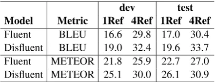
Showing the importance of fluent references for evaluation, Table5shows the performance of flu-ent models as evaluated on the original disfluflu-ent references. Disfluent target scores are the same as in Table2, and have been copied for easy

compar-dev test Model Metric 1Ref 4Ref 1Ref 4Ref

Fluent BLEU 16.6 29.8 17.0 30.4 Disfluent BLEU 19.0 32.4 19.6 33.7 Fluent METEOR 21.8 25.9 22.7 27.0 Disfluent METEOR 25.1 30.0 26.1 30.9

ison. As we would expect, here there is a greater difference in scores. The fluent references have fewer long n-gram matches with disfluencies re-moved, lowering BLEU. The fluent model’s ME-TEOR scores suffer more than BLEU due to the recall calculation; recall on the disfluent references is lower because the fluent model does not produce many of the disfluencies (indeed filler words are not in the vocabulary when trained with the fluent references). Recall is reduced by∼14%with the fluent model, reflecting the approximate distribu-tion of disfluencies in the original data.

The differences in scores with these two metrics do not show the full picture. Outputs generated by the fluent model are on average 13% shorter and contain 1.5 fewer tokens per utterance than the disfluent model, which is significant with av-erage utterance lengths of 10-11 tokens. When scoring the fluent output against the original dis-fluent references, the shorter length significantly contributes to the lower scores, with the BLEU brevity penalty calculated as 0.86 as opposed to 0.96-1.0 for all other conditions. Removing the length penalty from the BLEU score calculation, single-reference scores are boosted to 19.3 and 19.8 from 16.6 and 17.0 for dev and test, respectively (Table5). This is a somewhat fairer comparison of the disfluent and fluent models, as we do not want the fluent output to match the disfluent sequence length, and the disfluent models are not penalized due to length. These BLEU scores are now very similar to those of the disfluent model on the disflu-ent references, though the outputs are very differdisflu-ent (Figure1). The changes here and the difference in trends between the two metrics with respect to the two types of references show that evaluating this task cannot be simply accomplished with one exist-ing metric: dependexist-ing on the combination of metric and references, it’s possible to mask the difference between disfluent and fluent systems, unless you have word-level disfluency annotations, which are more difficult to obtain.

5 Conclusion

Machine translation applications for speech can suffer due to conversational speech phenomena, particularly the presence of disfluencies. Previous work to remove disfluencies in speech translation did so as a separate step between speech recogni-tion and machine translarecogni-tion, which is not possible using end-to-end models. Using clean references

for disfluent data collected bySalesky et al.(2018), we extend their text baseline to speech input and provide first results for direct generation of fluent text from noisy disfluent speech.

While fluent training data enables research on this task with end-to-end models, it is unlikely to have this resource for every corpus and domain and it is expensive to collect. In future work, we hope to reduce the dependence on fluent target data during training through decoder pretraining on external non-conversational corpora or multitask learning. Further, standard metrics alone do not tell the full story for this task; additional work on evaluation metrics may better demonstrate the differences be-tween such systems.

References

Sameer Bansal, Herman Kamper, Karen Livescu, Adam Lopez, and Sharon Goldwater. 2018. Low-resource speech-to-text translation. Proc. of Inter-speech. ArXiv:1803.09164.

Susanne Burger, Victoria MacLaren, and Hua Yu. 2002. The isl meeting corpus: The impact of meeting type on speech style.

William Chan, Navdeep Jaitly, Quoc Le, and Oriol Vinyals. 2016. Listen, attend and spell: A neural network for large vocabulary conversational speech recognition. In Acoustics, Speech and Signal Pro-cessing (ICASSP), 2016 IEEE International Confer-ence on, pages 4960–4964. IEEE.

Eunah Cho, Sarah F¨unfer, Sebastian St¨uker, and Alex Waibel. 2014. A corpus of spontaneous speech in lectures: The kit lecture corpus for spoken language processing and translation.

Eunah Cho, Thanh-Le Ha, and Alex Waibel. 2013. Crf-based disfluency detection using semantic features for german to english spoken language translation.

Michael Denkowski and Alon Lavie. 2014. Meteor uni-versal: Language specific translation evaluation for any target language.

Yarin Gal and Zoubin Ghahramani. 2016. A theoret-ically grounded application of dropout in recurrent neural networks.

David Graff, Shudong Huang, Ingrid Carta-gena, Kevin Walker, and Christopher Cieri. Fisher spanish speech (LDC2010S01). Https://catalog.ldc.upenn.edu/ ldc2010s01.

Matthias Honal and Tanja Schultz. 2005. Auto-matic disfluency removal on recognized sponta-neous speech-rapid adaptation to speaker-dependent disfluencies.

Diederik P Kingma and Jimmy Ba. 2015. Adam: A method for stochastic optimization. Proc. of ICLR. ArXiv:1412.6980.

Philipp Koehn, Hieu Hoang, Alexandra Birch, Chris Callison-Burch, Marcello Federico, Nicola Bertoldi, Brooke Cowan, Wade Shen, Christine Moran, Richard Zens, et al. 2007. Moses: Open source toolkit for statistical machine translation.

Gaurav Kumar, Matt Post, Daniel Povey, and Sanjeev Khudanpur. 2014. Some insights from translating conversational telephone speech.

Adrien Lardilleux and Yves Lepage. 2017. Charcut: Human-targeted character-based mt evaluation with loose differences. Proc. of IWSLT.

Minh-Thang Luong, Hieu Pham, and Christopher D. Manning. 2015. Effective approaches to attention-based neural machine translation.

Graham Neubig, Matthias Sperber, Xinyi Wang, Matthieu Felix, Austin Matthews, Sarguna Pad-manabhan, Ye Qi, Devendra Singh Sachan, Philip Arthur, Pierre Godard, et al. 2018. Xnmt: The extensible neural machine translation toolkit.

arXiv:1803.00188.

Toan Q Nguyen and David Chiang. 2018. Improving lexical choice in neural machine translation. Proc. of NAACL HLT. ArXiv:1710.01329.

Kishore Papineni, Salim Roukos, Todd Ward, and Wei-Jing Zhu. 2002. Bleu: a method for automatic eval-uation of machine translation.

Matt Post, Gaurav Kumar, Adam Lopez, Damianos Karakos, Chris Callison-Burch, and Sanjeev Khu-danpur. 2013. Improved speech-to-text translation with the fisher and callhome spanish–english speech translation corpus.

Daniel Povey, Arnab Ghoshal, Gilles Boulianne, Lukas Burget, Ondrej Glembek, Nagendra Goel, Mirko Hannemann, Petr Motlicek, Yanmin Qian, Petr Schwarz, et al. 2011. The kaldi speech recognition toolkit.

Elizabeth Salesky, Susanne Burger, Jan Niehues, and Alex Waibel. 2018. Towards fluent translations from disfluent speech.Proc. of SLT.

Matthias Sperber, Jan Niehues, Graham Neubig, Se-bastian St¨uker, and Alex Waibel. 2018. Self-attentional acoustic models. Proc. of EMNLP. ArXiv:1803.09519.

Christian Szegedy, Vincent Vanhoucke, Sergey Ioffe, Jon Shlens, and Zbigniew Wojna. 2016. Rethinking the inception architecture for computer vision.

Wen Wang, Gokhan Tur, Jing Zheng, and Necip Fazil Ayan. 2010. Automatic disfluency removal for im-proving spoken language translation.

Ron J Weiss, Jan Chorowski, Navdeep Jaitly, Yonghui Wu, and Zhifeng Chen. 2017. Sequence-to-sequence models can directly transcribe foreign speech. arXiv:1703.08581.

Vicky Zayats, Mari Ostendorf, and Hannaneh Hajishirzi. 2016. Disfluency detection us-ing a bidirectional lstm. Proc. of Interspeech. ArXiv:1604.03209.

Yu Zhang, William Chan, and Navdeep Jaitly. 2017. Very deep convolutional networks for end-to-end speech recognition.

A Appendix. LSTM/NiN Encoder and Training Procedure Details

A.1 Encoder Downsampling Procedure

Weiss et al.(2017) andBansal et al.(2018) use two strided convolutional layers atop three bidirectional long short-term memory (LSTM) (Hochreiter and Schmidhuber,1997) layers to downsample input sequences intime by a total factor of 4. Weiss et al.(2017) additionally downsamplefeature di-mensionality by a factor of 3 using a ConvLSTM layer between their convolutional and LSTM layers. This is in contrast to the pyramidal encoder (Chan et al., 2016) from sequence-to-sequence speech recognition, where pairs of consecutive layer out-puts are concatenated before being fed to the next layer to halve the number of states between layers.

To downsample in time we instead use the LSTM/NiN model used inSperber et al. (2018) andZhang et al.(2017), which stacks blocks con-sisting of an LSTM, a network-in-network (NiN) projection, layer batch normalization and then a ReLU non-linearity. NiN denotes a simple linear projection applied at every timestep, performing downsampling by a factor of 2 by concatenating pairs of adjacent projection inputs. The LSTM/NiN blocks are extended by a final LSTM layer for a total of three BiLSTM layers with the same to-tal downsampling of 4 asWeiss et al.(2017) and

Bansal et al.(2018). These blocks give us the ben-efit of added depth with fewer parameters.

A.2 Training Procedure