Using Multi Sense Vector Embeddings for Reverse Dictionaries

Using Multi-Sense Vector Embeddings for Reverse Dictionaries

Michael A. Hedderich1, Andrew Yates2, Dietrich Klakow1and Gerard de Melo3

1_{Spoken Language Systems (LSV), Saarland Informatics Campus, Saarbr¨ucken, Germany} 2_{Max Planck Institute for Informatics, Saarland Informatics Campus, Germany}

3_{Rutgers University, New Brunswick, NJ, USA}

{mhedderich, dietrich.klakow}@lsv.uni-saarland.de, [email protected], [email protected]

Abstract

Popular word embedding methods such as word2vec and GloVe assign a single vector represen-tation to each word, even if a word has multiple distinct meanings. Multi-sense embeddings instead provide different vectors for each sense of a word. However, they typically cannot serve as a drop-in replacement for conventional single-sense embeddings, because the correct sense vector needs to be selected for each word. In this work, we study the effect of multi-sense embeddings on the task of reverse dictionaries. We propose a technique to easily integrate them into an existing neural network architecture using an attention mechanism. Our experiments demonstrate that large improvements can be obtained when employing multi-sense embeddings both in the input sequence as well as for the target representation. An analysis of the sense distributions and of the learned attention is provided as well.

1

Introduction

One problem with popular word embedding methods such as word2vec (Mikolov et al., 2013) and GloVe (Pennington et al., 2014) is that they assign polysemic or homonymic words the same vector representa-tion, i.e., words that share the same spelling but have different meanings obtain the same representation. For example, the word “kiwi” can signify either a green fruit, a bird or, in informal contexts, the New Zealand dollar, which are three semantically distinct concepts. If only a single vector representation is used, then this representation is likely to primarily reflect the word’s most prominent sense, while ne-glecting other meanings (see Figure 1). More generally, a word vector may be a linear superposition of features of multiple unrelated meanings (Arora et al., 2018), resulting in incoherent vector spaces.

In recent years, several ideas have been proposed to overcome this problem. They have in common that they obtain different vector representations for the different meanings of polysemes or homonyms. Most prior work only evaluates these multi-sense vectors on single word benchmarks, however, and there is comparably little evidence for the benefits of using these embeddings in other applications.

kiwi

fruit banana

papaya pear_lemon guava

kiwifruit

bird emu tui bellbird kiwi chick NZD

greenback

(a)

lender_banker depositor

money shoreline riverside riverbank streambank

creek

bank

(b)

Figure 1: 2D projections of Google News word2vec vectors using t-SNE (Maaten and Hinton, 2008). The vector for the wordkiwiis located near the embedding for the New Zealand dollar (violet) and not near other birds (blue) or fruits (green). For bank, the vector lies in a neighborhood of financial terms (blue), further apart from other river related terms (green).

w

es(wi)

w

d

d

w

em(wi)

w

d

d

d

d

d

Figure 2: Single-sense embedding es compared to multi-sense embeddingemfor a sequence of input wordsw1,w2.

2

Task and Architecture

In this section, we give further details on the different embeddings, the reverse dictionary task and the corresponding architecture. We also motivate the use of multi-sense embeddings for the target and input vectors with qualitative examples and a quantitative analysis.

2.1 Single- and Multi-Sense Word Embeddings

A single-sense word embeddingesmaps a word or token to anl-dimensional vector representation, i.e.

es(wi) = di ∈ Rl for a wordwi. They are often pre-trained on large amounts of unlabeled text and

serve as a fundamental building block in many neural NLP models. Popular word embeddings include word2vec, GloVe and fastText (Bojanowski et al., 2017). If a word has several meanings, these are still mapped to just a single vector representation.

Multi-sense word embeddings emovercome this limitation by mapping each word wi to a list of sense vectors em(wi) = (di1, ...,dik), wherekis the number of senses that one considers wi to have. The

vectordij then represents one sense of the given word. This difference is visualized in Figure 2. Often,

these embeddings can also be pre-trained on unlabeled text. A discussion of different multi-sense word embeddings is given in Section 5.

2.2 Reverse Dictionaries

word (Zock and Bilac, 2004). We create a dataset for this task using the WordNet resource (Miller, 1995). For each word sense in this lexical database, we consider the provided gloss description as the input, and the word as the target.

the size of something as given by the distance around it→circumference

More details about the dataset are given in Section 4.1. Hill et al. (2016) presented a neural network approach for this task and also set it in the wider context of sequence embeddings. Each instance consists of a description, i.e. a sequence of words(w1, ..., wn), and a target vector t. Each word of the input sequence wi is mapped with a single-sense word embedding function es (e.g. word2vec) to a vector representationes(wi). This sequence of vectors is then transformed into a single vector

ˆ_{t=f(es(w1), ..., es(wn)). (1)}

Forf, the authors use—among others—a combination of an LSTM (Hochreiter and Schmidhuber, 1997) and a dense layer. The network is trained with the cosine loss betweentandˆt. During testing or when employed by a user, the model produces a ranking of the vocabulary words(α1, ..., α|V|)by comparing the vector representationes(αi)of each vocabulary wordαi with the predictionˆtin terms of the cosine

similarity measure. Thekmost similar words are returned to the user. We choose this task and architec-ture to show which benefits multi-sense vectors can bring to a downstream application and how they can easily be incorporated into an existing architecture. Two major limitations of single-sense vectors in this approach are presented in the following two subsections.

2.3 Target Vectors

The first limitation is that of the target vector, as exposed in Figure 1b. For the single-sense embedding, the vector for bank lies in a neighborhood consisting of financial terms with words such as banker, lender andmoney. Given a description of a river bankas input (the slope beside a body of water), a model trained on single-sense vectors as targets would have to produce a vectort(red point) that resides in a region of the semantic space that relates to financial institutions (blue points), rather than to nature and rivers (green points) with terms such asriversideorstreambank.

In Figure 3a, we observe that 68% of the target words in our training data have more than one possible sense in WordNet. While the sense distinctions in WordNet tend to be rather fine-grained, this shows that in general the phenomenon of encountering multiple senses for a target word is not limited to only a few instances but affects a large portion of the data.

To cope with this, we propose to rely on multi-sense vectors for the targett. Using these, we can assign the vector corresponding to the correct sense to each target in the training data. During testing, the correct target sense should obviously not be known to the model. We hence use for the ranking a vocabulary that consists of all sense vectors of all words.

2.4 Input Vectors

1 2 3 4 5 6 7 8 9 10 11 12 13 14 15 16 17 18 1920+ number of possible senses

0.00 0.05 0.10 0.15 0.20 0.25 0.30

fraction in training data

(a) Target words

0 1 2 3 4 5 6 7 8 9 10 11 12 13 14 15 16 17 18 1920+ number of possible senses

0.0 0.1 0.2 0.3 0.4

fraction in training data

(b) Description words

Figure 3: Number of possible senses, according to WordNet (see Section 4.2), of the target words (left) and input words (rights) in the training data. Out-of-vocabulary words are listed as having 0 senses.

w

d

d

d

ai2

ai1

ai3

d

d

d

sum

v

context

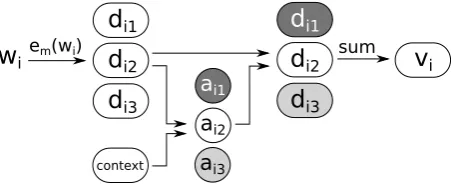
Figure 4: Visualization of the multi-sense vector selection using attention.

The analysis in Figure 3b shows that 38% of the words in the input sequence have more than one possible sense. This is a smaller percentage than in the case of target vectors, mostly due to out-of-vocabulary words and frequently occurring single-sense words such as stopwords. Nevertheless, this shows that multi-sense considerations are relevant for over a third of the words in the input definitions.

In contrast to the target vectors, we cannot directly link each input word to the correct sense vector be-cause annotating every description word with the corresponding sense would be very expensive. Instead, we propose to provide the model with all possible sense vectors for each description input word and to perform the selection directly within the neural network architecture in an end-to-end fashion. Our approach to achieve this in a differentiable way, employing an attention mechanism, is given in the next section.

3

Multi-Sense Vector Selection

The process of selecting multi-sense vectors is visualized in Figure 4. For an input sequence of words

(w1, ..., wn), first a representation of the context is computed. For this, a single-sense word embedding

functionesis used and an LSTM transforms this sequence into a context vectorc:

c=LSTM(es(w1), ..., es(wn))

For each wordwi, the multi-sense embedding functionemprovides one or more sense vectorsem(wi) =

rij =f(σ(c,dij)), (2)

where σ is a similarity function (dot product or cosine similarity in our case) and f is a non-linear function (ReLU in our experiments). The raw attention is normalized to yield attention weights

aij =

exp(rij) P

hexp(rih)

, (3)

and we obtain a new representation

vi = k X

j=1

aijdij. (4)

For each input word, instead ofes(wi), the vector vi is used in the task architecture. Equation 1 then

becomes

ˆ_{t=f(v1, ...,vn). (5)}

4

Experimental Evaluation

In the following, we will detail our experiments to evaluate the effect of multi-sense embeddings both for the input description and for the target words.

4.1 Data

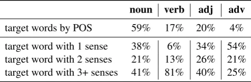
The dataset was created by extracting all single word lemmas from WordNet version 3.01. Each instance consists of a lemma as the target word and its corresponding definition as the description. We make this dataset publicly available2. When creating the data, we used an 80%/10%/10% train/dev/test split of the WordNet synsets. The data was split along synsets and not words to avoid any leakage of information from the test to the training data. For a fairer comparison with the single-sense baseline, we only used instances where the target word was in the vocabulary of the single-sense embedding. This resulted in 85,136 train, 10,521 development and 10,502 test instances. The descriptions were tokenized using SpaCy version 2.0.11 (Honnibal and Montani, 2017). The distribution of the part-of-speech tags of the target words is given in Table 1.

1

We do not use the original dataset by Hill et al. (2016) as it contains a flaw where a substantial part of the ”unseen” test instances are also part of the training data.

noun verb adj adv

target words by POS 59% 17% 20% 4%

target word with 1 sense 38% 6% 34% 54%

target word with 2 senses 21% 13% 26% 21%

target word with 3+ senses 41% 81% 40% 25%

Table 1: The first row shows the distribution of the part-of-speech tags (POS) of the target words in the dataset. The rest of the table contains the distribution of the number of senses, according to WordNet, given a specific POS.

4.2 Embeddings

In this work, we consider as our single-sense embedding es the popular 300-dimensional word2vec vectors trained on the Google News corpus3. For the multi-sense embeddingem, we chose the DeConf embeddings by Pilehvar and Collier (2016), which reside in the same space as the word2vec embeddings. It should be noted that DeConf uses the WordNetgraph structurefor the pre-training of the embeddings, while for our reverse dictionary data we only use the WordNetglossesas definitions.

4.3 Baselines

We compare our multi-sense approach that we introduced in the previous sections to the following baselines:

• For thesingle-sensebaseline, we use the reverse dictionary architecture proposed by Hill et al. (2016), which also serves as the foundation of all the multi-sense models.

• Infirst multi-sense, we experiment with using the first multi-sense vector for every word as a single-sense vector, i.e.vi =di1. This is motivated by the fact that the WordNet-based multi-sense vectors tend to be roughly ordered by frequency of occurrence (see analysis in Section 4.7).

• Random multi-senseevaluates using a randomly selected multi-sense vector.

• The modelnot-pretrainedis based on the approach of Kartsaklis et al. (2018). They recently proposed a method to obtain single-sense and multi-sense vector embeddings during training (in contrast to our use of pre-trained embeddings for both). While one of their experiments also evaluates on a reverse-dictionary setting, their results are unfortunately not directly comparable, as their targets are WordNet synsets and not words. We, therefore, integrate their proposed technique into our architecture in two ways: For the modelnot pre-trained, we use their equivalent version ofvi. This means that we use

their code for the training of the single and multi-sense embeddings as well as for the creation ofvi

based on the context and the multi-sense embedding. The modelonlyespre-traineddiffers from this

in that we use the pre-trained single-sense embedding instead of training it from scratch.

• TheBERTmodel belongs to the class of contextual word embeddings. This approach has been rapidly become popular with works by Peters et al. (2018), Radford et al. (2018), Peters et al. (2018b) and Devlin et al. (2018). Instead of using a direct mapping of words to vector representations, these approaches pre-train a neural language model on a large amount of text. The language model’s internal state for each input word is then used as a corresponding word vector representation for a different task. They can be viewed as inducing word vector representations that are specific to the surrounding context. We compare against the current state-of-the-art model BERT (Devlin et al., 2018). For this, the output of BERT’s last Transformer layer is used as the sequence(v1, ...,vn).

Input Vectors Target Vector MR↓ Acc@10↑ Acc@100↑ MRR↑

single-sense single-sense 535.5 0.115 0.301 0.067

single-sense multi-sense 135 0.203 0.458 0.131

multi-sense single-sense 481 0.121 0.315 0.069

multi-sense multi-sense 107 0.224 0.490 0.144

Table 2: Median rank, accuracy @10 and @100 and mean reciprocal rank of single- compared to multi-sense target vectors. The first row is the model architecture proposed by Hill et al. (2016).

4.4 Hyperparameters

We follow the choices of Hill et al. (2016) with an LSTM layer size of 512, a linear dense layer that maps to the size of the target vector and a batch size of 16. The input descriptions are clipped to a maximum length of 20 words and the number of senses per word is limited to 20. If a word does not exist in the multi-sense embedding, we fall back to the single-sense embedding. The pre-trained single and multi-sense word embeddings have a dimensionality of 300 and are fixed during training. For the embeddings created during training with the method of Kartsaklis et al., we experiment with the same dimensionality of 300 as well as with an embedding size of 150 (as suggested in their work). Apart from this, we follow the configuration of Kartsaklis et al. for their components. For the contextual BERT embeddings, the authors’ pre-trained, uncased model is used in the “base” and “large” variation and the pre-trained embeddings are again fixed. Since the BERT embeddings have a higher dimensionality (768 and 1024 respectively), the model architecture might underfit. We, therefore, experiment with different LSTM layer sizes up to 5,120, as well as with 2 LSTM layers and with adding a layer that transforms the embeddings to the same dimensionality of 300. For optimization, Adam (Kinga and Adam, 2015) is used for all models except foronlyespre-trained, which achieved better results using stochastic gradient descent with a fixed learning rate of 0.01.

4.5 Metrics

For evaluation, the vocabulary is ranked according to the cosine similarity of the produced vectorˆt as explained in Section 2.2. As the vocabulary, we use the union of all target words of the training, development, and test sets. Following Hill et al. (2016), we report the median rank as well as the mean accuracy @10 and @100. We also computed the mean reciprocal rank, which is a common metric in information retrieval.

4.6 Results

Input Vectors MR↓ Acc@10↑ Acc@100↑ MRR↑

single-sense (Hill et al., 2016) 135 0.203 0.458 0.131

first multi-sense 126 0.216 0.470 0.139

random multi-sense 137.5 0.208 0.457 0.136

not pre-trained 150 dim (Kartsaklis et al., 2018) 818 0.060 0.208 0.037

not pre-trained 300 dim (Kartsaklis et al., 2018) 574 0.087 0.260 0.053

onlyespre-trained 162 0.198 0.439 0.128

BERT base LSTM 512 (Devlin et al., 2018) 253.5 0.151 0.373 0.091

BERT base LSTM 4096 (Devlin et al., 2018) 183 0.181 0.423 0.109

BERT large LSTM 512 (Devlin et al., 2018) 249 0.156 0.375 0.093

BERT large LSTM 2048 (Devlin et al., 2018) 220 0.159 0.391 0.098

multi-sense (cosine similarity) 117 0.221 0.480 0.143

multi-sense (dot product similarity) 107 0.224 0.490 0.144

Table 3: Median rank, accuracy @10 and @100 and mean reciprocal rank for the experiments with different input vectors. The multi-sense vectors are used as target vectors.

In Table 3, we report the results for different approaches of handling the input vectors, as introduced in Sections 2.4 and 3. As target vectors, we use multi-sense vectors. Picking a random sense vector tends to perform slightly worse than using the single-sense vector embedding and both are outperformed by picking the first multi-sense vector of every word. This might be due to the fact that the first sense-vector tends to correspond to the most frequently occurring sense and that the representation of this sense is better in the multi-sense setting because it can focus on this meaning.

Using the same LSTM size of 512, the contextual BERT embeddings do not perform well. Adding a learnable linear or ReLU layer to transform them to a lower dimensionality or adding a second LSTM layer does not help either. Increasing the size of the LSTM improves performance until a certain point before it drops again. This might be due to a trade-off between the model underfitting and the learnability of the additional parameters. In the table, we report the best configuration for the ”base” and ”large” variation. In future work, it might also be interesting to experiment with fine-tuning the language model component of this architecture.

The model that uses the embedding training and multi-sense vector selection of Kartsaklis et al. seems to struggle with building good embeddings in this setting with the 300-dimensional embeddings performing somewhat better but still not well. Providing pre-trained single-sense embeddings improves the perfor-mance considerably. Although they are not trained task-specifically, the pre-training of the single-sense embeddings on large amounts of unlabeled data seems to result in a very useful embedding space. This is consistent with other works in the literature, e.g. Qi et al. (2018).

Our attention based multi-sense vector approach using pre-trained single- and multi-sense embeddings obtains the best results with respect to all four metrics, with the dot product similarity function perform-ing somewhat better than cosine similarity. This shows that usperform-ing pre-trained multi-sense vectors and selecting the right sense vectors can be beneficial in sequence embedding tasks.

4.7 Study of Senses and Attention

Model L

random multi-sense 0.25 first multi-sense 0.53

attention 0.31

attention-argmax 0.39

Table 4: Result of the analysis of the probability assigned to the true sense of multi-sense words for different models.

multi-sense embedding each word belongs. This data is made publicly available. Out of 275 words, 157 (57%) only had one vector representation, 18 words (7%) had a sense that was not covered by the corre-sponding multi-sense embedding entry, and 100 (37%) had one sense of the multiple possible meanings provided by the multi-sense embedding. On the latter, we calculated similarly to data likelihood the sum of the probabilities that different models assign to the correct sense:

L(m) =X w

pm(τ(w)|w), (6)

wheremis the model,wis a word andτ(w)is the true sense of the word. Forrandom multi-sense, the probability was the reciprocal of the number of senses of a word. Forfirst multi-sense, the probability was 1 if it was the first sense of a word in the multi-sense embedding and 0 otherwise. Forattention, we used the normalized attentionaof the true sense. Forattention-argmax, probability 1 was assigned to the sense that had the maximum attention. The results are given in Table 4.

As mentioned earlier, the first sense of the multi-sense embedding often reflects the dominant usage, being correct in about half of the cases. The attention approach suffers from the dilution that a soft attention entails. Due to the use of the soft-max function, all senses get at least a small amount of the probability mass. An attention mechanism that uses a more skewed probability distribution might be beneficial here. Fromattention-argmax, we see that the attention method also does not always assign the largest amount of attention to the correct sense. The fact that this architecture still outperforms the others can be explained by the compositional nature of the attention mechanism. Also, some of the senses in the DeConf multi-sense embeddings tend to be very fine-grained. This means that even if not the exact sense is given the most attention, a similar sense might be. For future work, it would be interesting to improve on the context creation and sense selection component, explore options to fine-tune the embeddings as well as experiment with other multi-sense embeddings that might have a smaller number of different senses per word.

5

Related Work

In recent years, several approaches to creating multi-sense vector embeddings have been proposed. Rothe and Sch¨utze (2015), Pilehvar and Collier (2016) and Dasigi et al. (2017) use an existing single-sense word embedding and a lexical resource to induce vectors representing different senses of a word. The latter also employ an attention-based approach for creating vectors based on the context for predicting prepositional phrase attachments. Pilehvar et al. (2017) use the same DeConf multi-sense embedding for integrating them in a downstream application. In contrast to our work, they require, however, a semantic network to do the disambiguation. In Sense2Vec (Trask et al., 2015), the authors create embeddings that distinguish between different meanings given the corresponding part-of-speech or named entity tag. They obtain an embedding that distinguishes e.g. between the location Washington and the person with the same name. The method requires the input data to be tagged with POS or NE tags. Athiwaratkun and Wilson (2017) represent multiple meanings as a mixture of Gaussian distributions. The number of senses per word is fixed globally to the number of Gaussian components. Raganato et al. (2017) and Pesaranghader et al. (2018) use bidirectional LSTMs to learn a mapping between words and multiple senses (not sense vectors) as a supervised sequence prediction task requiring sense-tagged text. An extensive survey on further ideas and work regarding vector representations of meaning is given by Camacho-Collados and Pilehvar (2018).

Tang et al. (2018) analyzed different attention mechanisms in the specific context of ambiguous words in machine translation. They limit their approach, however, to single-sense vectors and the established method of using attention over other parts of the sentence to improve the translation process.

6

Conclusion

In this work, we study the use of multi-sense vector embeddings for the reverse dictionary task. We show that single-sense embeddings such as word2vec do not adequately reflect all meanings of polysemes and homonyms and that improvements can be obtained by using multi-sense embeddings both for the target words and for the words in the input description. For the latter, we proposed a method based on attention that automatically selects the correct sense from a set of pre-trained multi-sense vectors depending on the context in an end-to-end fashion. It outperforms single-sense vectors, multi-sense embeddings trained in a task-specific way as well as pre-trained contextual embeddings. Our analysis of the sense selection process shows avenues for interesting future work.

Acknowledgment

The authors would like to thank the reviewers for their helpful comments. Michael Hedderich thankfully acknowledges the support by the obtained fellowship within the FITweltweit program of the German Academic Exchange Service (DAAD). Gerard de Melo’s research is in part supported by the Defense Advanced Research Projects Agency (DARPA) and the Army Research Office (ARO) under Contract No. W911NF-17-C-0098. Any opinions, findings and conclusions, or recommendations expressed in this material are those of the authors and do not necessarily reflect the views of the funding agencies.

References

Arora, S., Y. Li, Y. Liang, T. Ma, and A. Risteski (2018). Linear algebraic structure of word senses, with applications to polysemy.Transactions of the Association for Computational Linguistics 6, 483–495.

Bastos, A. (2018). Learning sentence embeddings using recursive networks. arXiv preprint arXiv:1810.04805.

Bojanowski, P., E. Grave, A. Joulin, and T. Mikolov (2017). Enriching word vectors with subword information. Transactions of the Association for Computational Linguistics 5, 135–146.

Bosc, T. and P. Vincent (2018). Auto-encoding dictionary definitions into consistent word embed-dings. InProceedings of the 2018 Conference on Empirical Methods in Natural Language Processing (EMNLP).

Camacho-Collados, J. and M. T. Pilehvar (2018). From word to sense embeddings: A survey on vector representations of meaning. Journal of Artificial Intelligence Research.

Dasigi, P., W. Ammar, C. Dyer, and E. Hovy (2017). Ontology-aware token embeddings for prepositional phrase attachment. InProceedings of the 55th Annual Meeting of the Association for Computational Linguistics (ACL).

Devlin, J., M.-W. Chang, K. Lee, and K. Toutanova (2018). Bert: Pre-training of deep bidirectional transformers for language understanding.arXiv preprint arXiv:1810.04805.

Hill, F., K. Cho, A. Korhonen, and Y. Bengio (2016). Learning to understand phrases by embedding the dictionary. Transactions of the Association for Computational Linguistics 4, 17–30.

Hochreiter, S. and J. Schmidhuber (1997). Long short-term memory. Neural computation 9(8), 1735– 1780.

Honnibal, M. and I. Montani (2017). spacy 2: Natural language understanding with bloom embeddings, convolutional neural networks and incremental parsing.

Kartsaklis, D., M. T. Pilehvar, and N. Collier (2018). Mapping text to knowledge graph entities using multi-sense lstms. InProceedings of the 2018 Conference on Empirical Methods in Natural Language Processing (EMNLP).

Kinga, D. and J. B. Adam (2015). Adam: A method for stochastic optimization. In International Conference on Learning Representations (ICLR), Volume 5.

Maaten, L. v. d. and G. Hinton (2008). Visualizing data using t-sne. Journal of machine learning research 9(Nov), 2579–2605.

Mikolov, T., K. Chen, G. Corrado, and J. Dean (2013). Efficient estimation of word representations in vector space. arXiv preprint arXiv:1301.3781.

Miller, G. A. (1995). Wordnet: a lexical database for english. Communications of the ACM 38(11), 39–41.

Pennington, J., R. Socher, and C. D. Manning (2014). Glove: Global vectors for word representa-tion. InProceedings of the 2014 Conference on Empirical Methods in Natural Language Processing (EMNLP).

Pesaranghader, A., A. Pesaranghader, S. Matwin, and M. Sokolova (2018). One single deep bidirectional lstm network for word sense disambiguation of text data. In E. Bagheri and J. C. Cheung (Eds.), Advances in Artificial Intelligence, Cham, pp. 96–107. Springer International Publishing.

Peters, M., M. Neumann, L. Zettlemoyer, and W.-t. Yih (2018b). Dissecting contextual word embed-dings: Architecture and representation. InProceedings of the 2018 Conference on Empirical Methods in Natural Language Processing (EMNLP).

Pilehvar, M. T., J. Camacho-Collados, R. Navigli, and N. Collier (2017). Towards a seamless integration of word senses into downstream nlp applications. InProceedings of the 55th Annual Meeting of the Association for Computational Linguistics (ACL).

Pilehvar, M. T. and N. Collier (2016). De-conflated semantic representations. InProceedings of the 2016 Conference on Empirical Methods in Natural Language Processing (EMNLP).

Qi, Y., D. Sachan, M. Felix, S. Padmanabhan, and G. Neubig (2018). When and why are pre-trained word embeddings useful for neural machine translation? In Proceedings of the 2018 Conference of the North American Chapter of the Association for Computational Linguistics: Human Language Technologies (NAACL-HLT).

Radford, A., K. Narasimhan, T. Salimans, and I. Sutskever (2018). Improving language understanding by generative pre-training. Technical report, OpenAI.

Raganato, A., C. Delli Bovi, and R. Navigli (2017). Neural sequence learning models for word sense disambiguation. InProceedings of the 2017 Conference on Empirical Methods in Natural Language Processing (EMNLP).

Rothe, S. and H. Sch¨utze (2015). Autoextend: Extending word embeddings to embeddings for synsets and lexemes. InProceedings of the 53rd Annual Meeting of the Association for Computational Lin-guistics (ACL).

Scheepers, T., E. Kanoulas, and E. Gavves (2018). Improving word embedding compositionality using lexicographic definitions. InProceedings of the 2018 World Wide Web Conference (WWW).

Tang, G., M. M¨uller, A. Rios, and R. Sennrich (2018). Why self-attention? a targeted evaluation of neural machine translation architectures. InProceedings of the 2018 Conference on Empirical Methods in Natural Language Processing (EMNLP).

Trask, A., P. Michalak, and J. Liu (2015). sense2vec-a fast and accurate method for word sense disam-biguation in neural word embeddings. arXiv preprint arXiv:1511.06388.