54
Language Discrimination and Transfer Learning for Similar Languages:
Experiments with Feature Combinations and Adaptation
Nianheng Wu Eric DeMattos Kwok Him So Pin-zhen Chen C¸ a˘grı C¸ ¨oltekin University of T¨ubingen
Department of Linguistics
{nianheng.wu|eric.demattos|kwok-him.so|pinzhen.chen}@student.uni-tuebingen.de [email protected]
Abstract
This paper describes the work done by team tearsofjoy participating in the VarDial 2019 Evaluation Campaign. We developed two systems based on Support Vector Machines: SVM with a flat combination of features and SVM ensembles. We participated in all language/dialect identification tasks, as well as the Moldavian vs. Romanian cross-dialect topic identification (MRC) task. Our team achieved first place in German Dialect identi-fication (GDI) and MRC subtasks 2 and 3, sec-ond place in the simplified variant of Discrim-inating between Mainland and Taiwan vari-ation of Mandarin Chinese (DMT) as well as Cuneiform Language Identification (CLI), and third and fifth place in DMT traditional and MRC subtask 1 respectively. In most cases, the SVM with a flat combination of features performed better than SVM ensem-bles. Besides describing the systems and the results obtained by them, we provide a ten-tative comparison between the feature combi-nation methods, and present additional exper-iments with a method of adaptation to the test set, which may indicate potential pitfalls with some of the data sets.
1 Introduction
Language identification is a text classification task that has been studied extensively in the field of Natural Language Processing. The general con-cept and common implementations are described
in the recent survey byJauhiainen et al.(2018c). A
more challenging task is discerning closely related languages or dialects of the same language. In re-cent years, the VarDial Evaluation Campaign has organized a multitude of shared tasks on
classify-ing these with textual and spoken data (Malmasi
et al., 2016; Zampieri et al., 2017, 2018). This
year’s VarDial evaluation campaign (Zampieri
et al.,2019) featured one rerun (Swiss German
di-alect identification) and three new closely-related language identification tasks (Mainland vs. Tai-wan varieties of Mandarin, Romanian vs. Molda-vian, and cuneiform language identification, with the latter covering seven related languages within a wide historical time frame). Our focus has been German dialect identification (GDI) and discrimi-nating between mainland and Taiwan varieties of Mandarin (DMT). However, we submitted predic-tions for all language identification tasks.
While closely-related languages (or dialects) pose a challenge for language identification, they also provide opportunities for cross-lingual trans-fer where available resource and tools in one lan-guage is adapted to another, similar lanlan-guage va-riety. This year’s evaluation campaign also
fea-tures two cross-lingual transfer tasks. Namely,
cross-lingual morphological analysis (CMA), and cross-lingual topic identification between Roma-nian and Moldavian (MRC). The CMA is a sub-stantially different task than language identifica-tion. However, the MRC subtasks on cross-lingual topic identification can be solved by the very same text classification models used for language iden-tification. Hence, we also participated in the cross-lingual classification subtasks of the MRC.
Our base model is a linear support vector ma-chine (SVM) classifier with sparse character and word n-gram features. These models have been found to be successful in earlier instances of Var-Dial language identification tasks; in fact, they were found to be more effective than more
re-cent neural classifiers (C¸ ¨oltekin and Rama,2016;
Clematide and Makarov,2017;Medvedeva et al.,
2017). A successful variation of these linear
clas-sifiers is an ensemble of clasclas-sifiers with different n-gram orders used both for language
discrimi-nation (Malmasi and Zampieri,2017b,a), and
na-tive language identification (Malmasi and Dras,
the overlapping n-gram features, we also used an ensemble approach in some of the tasks, providing a tentative comparison between these two related methods.
An interesting result of last year’s VarDial evaluation campaign was SUKI team’s success
on Indo-Aryan language identification (Jauhiainen
et al., 2018b) and GDI (Jauhiainen et al., 2018a) tasks with a rather large margin, which was likely because of the adaptation mechanism they used at prediction time. We adopted a similar adapta-tion approach to our SVM systems. Besides the curious difference in the GDI data set last year, the adaptation idea is also a good fit for the cross-lingual topic identification task (MRC).
The remainder of this paper introduces the tasks and data sets, describes our systems, and presents the results obtained followed by a brief discussion.
2 Tasks and Data
2.1 CLI: Cuneiform Language Identification
The provided datasets for Cuneiform Language
Identification (Jauhiainen et al., 2019) consisted
of a training set and a development set. The
training data contained cuneiform texts written in Sumerian (SUX) and six Akkadian dialects: Old Babylonian (OLB), Middle Babylonian peripheral (MPB), Standard Babylonian (STB), Neo Babylo-nian (NEB), Late BabyloBabylo-nian (LTB), and Neo As-syrian (NEA). The data for the shared task con-tained only Unicode transcriptions of the docu-ments without token boundaries or any other vi-sual features. The data set exhibited a large class
imbalance, ranging from 3 803 instances for Old
Babylonian to53 673instances for Sumerian. The
training data contained a total of139 421text
sam-ples, while the development set contained 668
lines for each language or dialect.
2.2 DMT: Discriminating between Mainland and Taiwan variation of Mandarin
The Discriminating between Mainland and Tai-wan variation of Mandarin Chinese (DMT) task consisted of classifying sentences extracted from news articles into classes of two major
Man-darin variations: Putonghua (Mainland China)
andGuoyu(Taiwan). The task has two tracks: tra-ditional and simplified.
In Mandarin Chinese, there are many
mutu-ally intelligible regional variations. Putonghua
and Guoyu are more distinguishable in spoken
language due to systematic phonetic differences, while they are more ambiguous in written text with no overt morphological, syntactic, and lexical preferences in language use, especially in formal text. It is considered challenging even for native speakers to distinguish between them, and since the shared task data offered only textual informa-tion with no phonetic transcripinforma-tion, it was partic-ularly interesting to explore possible solutions to the problem.
In contemporary written Chinese, there are two scripts: traditional and simplified. The only dis-tinction between the two writing systems is the visual form of the characters. As the name sug-gests, characters in simplified Chinese usually ap-pear simpler than their traditional counterparts, while some are identical which may lead to per-formance variations based on different system de-signs. A text in traditional Chinese can always be transformed verbatim into its simplified counter-part without any content change and vice versa. Two corpora, one using traditional script and one simplified, were provided to investigate the perfor-mance of the discrimination task on the two dif-ferent scripts, which will be further discussed in
Section5.
The DMT data comes from the news domain for both varieties. The datasets contained a train-ing and development set for both simplified
Chi-nese (McEnery and Xiao, 2003) and traditional
Chinese (Chen et al., 1996). The training set
consisted of18 770samples for both Chinese
va-rieties, whereas the development set contained
2 000samples each. The texts contained no punc-tuation and were (automatically) segmented by the task organizers.
2.3 GDI: German Dialect Identification
As in previous years, the GDI data set is based on
the corpus introduced inSamardˇzi´c et al. (2016),
consisting of samples from four regions around Bern (BE), Basel (BS), Lucerne (LU) and Zurich (ZH). Besides transcriptions of the audio record-ings, we were also provided with 400-dimensional i-vectors representing the acoustic features of each sample, and automatically obtained normalization data where words are paired with their standard German spelling. In our submissions, we used the text transcripts and i-vectors.
There were 14 279training and4 530
sets included a fair amount of class imbalance.
2.4 MRC: Moldavian vs. Romanian Cross-dialect Topic identification
The MRC task involved discrimination between two closely written language varieties, Romanian and Moldavian, and cross-variety topic classifica-tion. The first subtask was a binary classification problem, discriminating between the two language varieties. The second and third tasks required clas-sifying the documents in one variety using training data from the other variety into six topics: culture, finance, politics, science, sports and technology. The second subtask used Moldavian as the source language and Romanian as the target language in the transfer task. Task 3 had the same setup, but the source and target languages were swapped. Topic classification tasks are formulated as multi-class problems (in contrast to multi-label multi- classi-fication common in the field), where each text is assigned to only one class. Named entities in the data set were anonymized.
The training data for subtask 1 consisted of
21 701texts with a slight class imbalance (11 740
Romanian,9 961Moldavian), with a development
set of 11 834 instances approximately following
the same class distribution. Training sets for
sub-tasks 1 and 2 included9 961and11 740texts, and
development sets included5 432 and 6 402 texts,
respectively. All subtasks shared a test set of5 918
texts, although subtasks 2 and 3 were evaluated on subsets of the test set. Further information on the
data can be found inButnaru and Ionescu(2019).
3 Methods and experimental setting
Our main submissions were based on two SVM systems that differ in the way they combine the n-gram features: SVM with flat feature combina-tions and SVM ensembles. We employed both
character and word n-gram features.
Depend-ing on the task, the character n-grams varied be-tween 1 to 9 and the word n-grams varied from 1 to 3. The features were weighted with either
tf-idf or BM25 (Robertson et al., 2009)
weight-ing schemes. The flat combination is similar to
C¸ ¨oltekin and Rama(2016) and the ensemble
ap-proach is similar to Malmasi and Dras (2015).
Both methods were implemented in Python using
the scikit-learn library (Pedregosa et al.,2011).
We also experimented with recurrent neural classifiers and considered a system similar to HeLi
(Jauhiainen et al.,2016), which was also used in earlier VarDial evaluation campaigns. However, we only submitted results with the SVM classi-fiers described in more detail below, and we will limit our discussion to the results obtained by the SVM classifiers.
3.1 SVM with flat combinations of features
For all tasks, we submitted predictions generated by SVM classifiers where a range of overlapping character and word n-grams are combined into a single feature matrix. The features are weighted using BM25, although a plain tf-idf weighing scheme produced similar results on the develop-ment set. In all tasks, we optimized the model hyperparameters through random search, using 5-fold cross validation on combined training and de-velopment sets. Random search was stopped
af-ter approximately 1 000 draws from the space of
random parameters, and picking the best average
F1-score over the5folds. This is simply the same
approach taken in a series of earlier VarDial
evalu-ation campaigns (C¸ ¨oltekin and Rama,2016;Rama
and C¸ ¨oltekin, 2017; C¸ ¨oltekin and Rama, 2017;
C¸ ¨oltekin et al.,2018).
Following the adaptation idea used by
Jauhi-ainen et al.(2018a,b) in last year’s VarDial eval-uation campaign, we also employed an adaptation approach in some of the tasks. At test time, we produced a set of first-level predictions based on the best model tuned for the task on the train-ing/development set, and retrained the model af-ter adding the predictions with high-confidence to the training set. In our case, predictions with high-confidence means the test instances that are
farther than a threshold — in this case, 0.50 —
from the decision boundary for binary classifica-tion, and the instances that are claimed by only one of the one-vs-rest classifiers for the multi-class problems. Intuitively, this is useful for the adapta-tion subtasks of MRC, and in case the distribuadapta-tion of the test instances diverge from the distribution in the training/development sets.
All tasks we participated in involved text
clas-sification. However, the GDI data set also
by BM25, before feeding them to the SVM
clas-sifiers. As SVMs are sensitive to the scale of
the data, we introduced a weight parameter and searched for its optimum value during tuning.
3.2 SVM ensembles
SVM ensembles are generally considered more
ro-bust than single classifiers (Oza and Tumer,2008).
An ensemble system makes use of decisions from multiple classifiers on every input entity. The deci-sions are congregated through a fusion method, re-evaluated, and a final decision is made. There are
various fusion methods (Malmasi and Dras,2015),
but the one we chose was mean probability rule,
an approach that is considered stable and simple (Kuncheva, 2004) as well as resistant to
estima-tion errors (Kittler,1998). Each classifier returns
a prediction with the probability of each test in-stance belonging to each label. The final decision is the label with the highest average probability.
Each classifier was trained on the standard train-ing set ustrain-ing strain-ingle n-gram order. We performed binary search on the DMT simplified training de-velopment set in the range of [0, 1000] in order to determine the ideal penalty value C. The F1-score increased with increasing C value, and plateaued
when C≥100, so we adopted C =100as the
opti-mal value. Table2lists the score of each classifier
using the DMT simplified development set.
Since SVMs separate classes by maximizing
the margin from items to the hyperplane (Burges,
1998), there is no natural probabilistic
interpreta-tion of the decision funcinterpreta-tion of an SVM classi-fier. Therefore, we applied the technique of
cal-ibration suggested byPlatt et al.(1999), a method
that maps the outputs of SVM to probabilities, as implemented in the scikit-learn library.
We used grid search to find the optimal combi-nation of n-gram features for each task. For DMT simplified, the final ensemble system we selected utilized five parallel classifiers, each of them gen-erated with different parameters: character-based bigrams, trigrams, 4-grams, 5-grams, and word-based unigrams. For DMT traditional, the com-bination additionally included character-based
un-igrams. For GDI, we used character-based
bi-grams, tribi-grams, 4-bi-grams, 5-bi-grams, word-based unigrams, and the audio i-vectors.
task (model) F1-macro rank F1-diff
DMT-S (flat) 87.38 2 −1.91
DMT-S (ens.) 84.45 NA −4.84
DMT-T (flat) 88.44 3 −2.41
DMT-T (ens.) 85.61 NA −5.24
GDI (flat) 75.93 1 0.52
GDI (ens.) 65.17 NA −10.76
MRC 1 (flat) 75.73 5 −13.92
MRC 2 (flat) 61.15 1 5.26
MRC 3 (flat) 55.33 1 13.23
MRC 1 (flat)∗ 96.20 NA 6.70
MRC 2 (flat)∗ 69.08 NA 7.93
MRC 3 (flat)∗ 81.93 NA 26.60
CLI (flat) 76.32 2 −0.63
Table 1: Official results obtained by our models on all tasks we participated. The column F1-diff indicates the macro F1-score difference from the top score if the result is not the top score, or the difference from the second best scores otherwise. Our submissions in the MRC task had an error, causing a shift of labels after a certain index. The scores marked with ∗ are post-evaluation results with the gold labels released by the organizers after the evaluation period.
4 Results
We list the results obtained by our systems on the
official test sets in Table 1. The results clearly
show that the simple linear classifiers we used are competitive with other (best) participating sys-tems. Furthermore, in our experiments, the flat combination often worked better than the ensem-ble method. However, we do not provide a more conclusive, systematic comparison at this time. In the remainder of this section, we will first de-scribe some of the interesting results in each task, and also present a series of additional experiments with the adaptation method described above.
4.1 DMT
For both DMT tasks, we submitted at least one classifier with a combined feature matrix (flat) and at least one model with parallel classifiers (ensem-ble). Our submissions with a combined feature matrix using character n-grams of order 1 to 4 combined with word unigrams and bigrams con-sistently outperformed the parallel classifiers.
on the order of approximately 87–89 % accuracy with no significant jump in accuracy using any particular combination. However, the most gains were observed when combining a large number of
character n-grams with1 ≤n ≤5and word
uni-grams. Word bigrams already resulted in a signif-icant loss of accuracy in the SVM ensemble (pos-sibly overfitting due to large number of features, and large C value selected in the earlier step).
Feature Types n F1 macro
character 1 77.41
character 2 83.77
character 3 87.19
character 4 86.99
character 5 83.75
word 1 76.63
[image:5.595.308.530.172.368.2]word 2 33.33
Table 2: F1 scores achieved by SVM with single fea-tures, tested on development set (Simplified Chinese)
During development, we observed that train-ing and testtrain-ing our model on traditional Chinese consistently performed slightly better than training and testing on simplified Chinese. Combining the traditional training set with the simplified training set did not yield any significant gains and in fact slightly hindered the model’s performance.
Our flat SVM model placed second for simpli-fied and third for traditional. Other teams also saw higher F1-scores for traditional compared to sim-plified which suggests that the traditional script carries more information that proves useful in
dis-tinguishing between the two dialects. Despite
this, our model misidentified the Taiwanese vari-ant roughly twice as often as its Mainland
coun-terpart using both scripts (simplified: 166vs. 88,
traditional:151vs.80).
4.2 GDI
The same models used for DMT were slightly modified for the German Dialect Identification task. Our flat model using character n-grams of order 1 to 5, word unigrams and bigrams, and the i-vector features achieved first place with an
F1-score of75.93, which was very closely followed
by the second and third place entries.
The confusion matrix presented in Figure 1
demonstrates that Basel was most easily identified
(recall: 91.99). Lucerne was the dialect most
of-ten misclassified (recall:62.41), usually confused
with Bern. Consequently, Bern had the lowest
pre-cision (69.39) while Basel and Zurich enjoyed the
highest (tied with80.81). This distribution mirrors
the results of last year’s GDI task (Ciobanu et al.,
2018;Ali, 2018; Benites et al., 2018; Barbaresi,
2018).
BE BS LU ZH
Predicted label BE
BS
LU
ZH
True label
943
30
110
108
22
1103
33
41
358
34
734
50
36
198
105
838
Confusion Matrix
[image:5.595.105.257.202.324.2]0.0 0.2 0.4 0.6 0.8
Figure 1: Confusion matrix for GDI. Abbreviation key: Bern (BE), Basel (BS), Lucerne (LU), Zurich (ZH).
In the development set, the SVM ensemble with
character n-grams of2 ≤n ≤5, word unigrams,
and audio i-vectors outperformed the flat feature combination. The ensemble system yielded an
F1-score of65.35in comparison to a44.24F1-score
obtained by the flat combination. This is likely due to the fact that ensemble systems are partic-ularly effective when the individual classifiers are independent, and features from text and audio pro-vide more independent predictions in comparison
to the overlapping n-gram features.1
4.3 CLI
We submitted predictions using only the flat fea-ture combination for the cuneiform language iden-tification task. Our submission with adaptation
came in a close second with an F1-score of76.32.
Since the data did not include any word bound-aries, our system combines only character n-grams
(of order1to5). We also experimented with two
unsupervised segmentation methods (C¸ ¨oltekin and
Nerbonne,2014;Virpioja et al.,2013). However,
using tokens obtained through both segmentation methods as (additional) features did not improve the results on the development set.
On the CLI data, the adaptation method is highly effective. Our submission with no
adapta-tion performed much worse (53.18F1-score). We
will present more results with adaptation in
Sec-tion4.5and discuss it further in Section5.
The confusion matrix from our official
submis-sion is presented in Figure2, which depicts some
effects of the historical proximity of the languages.
LTB MPB NEA NEB OLB STB SUX
Predicted label LTB
MPB
NEA
NEB
OLB
STB
SUX
True label
942
13 2
1
23 4
6
825 44 15 22 38 35
4
7
890 44 1
20 19
22 36 212 593 4
94 24
23 39 71 12 736 37 67
17 28 206 128 17 516 73
6
10 37 8
52 99 773
Confusion Matrix
[image:6.595.76.295.236.432.2]0.0 0.2 0.4 0.6 0.8
Figure 2: Confusion matrix for CLI. Abbreviations: Late Babylonian (LTB), Middle Babylonian peripheral (MPB), Neo Assyrian (NEA), Neo Babylonian (NEB), Old Babylonian (OLB), Standard Babylonian (STB), Sumerian (SUX).
4.4 MRC
We submitted predictions with only the flat com-bination for the MRC tasks. Our submissions in this task had an error, causing a shift of labels af-ter a certain index. Despite this shift (with some effort from the organizers to guess the location of the missing predictions) our submissions ob-tained first rank in subtasks 2 and 3. After rectify-ing the problem post-evaluation, F1-macro scores
increased by up to 30%, reaching 96.20 for
sub-task 1,69.08in subtask 2, and81.93in subtask 3.
The high rate of success in discriminating between such close linguistic varieties is interesting. How-ever, the primary objective in MRC was cross-lingual learning in the last two subtasks which we
discuss further in Section4.5.
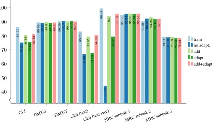
4.5 Adaptation to target data
In this instance of the VarDial evaluation cam-paign, we employed a method of adaptation to the test data. Among the tasks in which we partici-pated, the clear cases for adaptation are MRC sub-tasks 2 and 3. These sub-tasks are transfer learning tasks, hence some sort of adaptation is expected to help. In other cases, we do not expect substantial gains from adaptation unless test sets diverge from the training substantially and systematically.
Our official submissions did not always include results from the identical models with and without adaptation, and as such does not clearly indicate the utility of it. Here, we present results from more systematic experiments conducted on the develop-ment sets using our SVM model with flat combi-nations of features. The intuition here is that if the distribution of the test instances diverge from the training set, we can adapt to the test set either by using a small amount of data with gold-labels, or predictions with high confidence at prediction time. The first method (adding gold target data) is not an option during the shared task evaluation. Therefore, we tested both options on the desig-nated development sets. For the second method (adaptation at prediction time), our method is
sim-ilar to, but simpler than, the method ofJauhiainen
et al. (2018a,b). We trained a base classifier on the training data, and re-trained the system af-ter adding the test instances predicted with high-confidence to the training data. For binary tasks, we picked the training instances with a distance
greater than 0.50 to the decision boundary. For
multi-class classification problems, we picked the instances that are claimed by only one of the one-vs-rest classifiers as confident predictions.
Figure 3 presents five sets of results on all
CLI DMT-S
[image:7.595.78.509.63.316.2]DMT-T GDI(text) GDI(text+v ec) MRCsubtask 1 MRCsubtask 2 MRCsubtask 3 40 50 60 70 80 90 100 86 . 59 89 . 59 90 . 39 83 . 23 99 . 48 95 . 08 90 . 59 79 . 54 75 . 05 89 . 2 90 . 7 66 . 89 44 . 24 95 . 77 92 . 35 79 . 12 80 . 88 89 . 9 90 . 4 79 . 65 94 95 . 88 93 . 25 79 . 19 75 . 82 89 . 2 90 . 7 67 . 68 79 . 65 95 . 74 92 . 19 78 . 54 81 . 42 89 . 6 90 . 3 80 . 92 95 . 63 95 . 84 92 . 3 78 . 62 train no adapt. add adapt add+adapt
Figure 3: Results of adaptation experiments. The graph presents macro averaged F1-scores of five experiments on each task. ‘train’ indicates average of 5-fold CV on training set; ‘no adapt.’ indicates no adaptation, train only on the training set; ‘add’ indicates adding half of the gold-labeled data from the development set, and testing on the other half; ‘adapt’ is adaptation during training by adding predictions with high-confidence to the training set and re-training the model; and ‘add+adapt’ combines the last two options.
a large amount of data from the source domain, with a small amount of data from the target do-main. The training instances from the source and target are equally weighted in our experiments. In the fourth set of experiments (adapt), the base clas-sifier is trained on the training data, and testing is done adaptively on the second part of the develop-ment set. The final bar (add+adapt) combines the last two. The base system is trained with the com-bination of the training set and the first half of the development set, and tested on the second part of the development set using adaptation.
The scores illustrated in Figure3for both DMT
tasks and MRC subtask 1 (language identification) are as expected. The cross-validation scores on the training set are slightly better than scores on the test (part of official development) set, and adap-tion opadap-tions give a slight boost in most cases. In MRC subtask 2, the F1-score on the test set is bet-ter than the training set. This is particularly inbet-ter- inter-esting, as this is a language transfer task where the test set is expected to diverge. All scores we ob-tained in this subtask are also much higher than the
(corrected) official test set score (69.08) presented
in Table1. Adaptation, however, seems to help if
data with gold labels are added. In MRC subtask
3, which reverses the languages in MRC subtask 2, adaptation does not seem to be useful either.
The results of CLI and, especially, GDI tasks are particularly surprising. In these tasks, adap-tation, and especially the addition of gold-labeled data, seem to improve the results drastically. The difference likely indicates a systematic difference between the training and development sets (and possibly test). We provide further discussion of
these results for the GDI, in Section5.
5 Summary and Discussion
DMT task, and discuss the potential reasons for the effectiveness of adaptation methods.
Observations on the DMT task. The relation-ship from traditional Mandarin to simplified is generally bijective, but there are some cases where
the relation is many-to-one. Thus, a machine
is better able to predict using traditional over simplified. Consequently, this explains why our model always produced 1-2% better results with
the traditional script. To illustrate this,
con-sider the following example: 「雲」‘cloud’ and
「云」‘speak’ in traditional Mandarin are both
written as 「云」in simplified, which indicates
that the simplified character「云」carries the
meaning of both ‘cloud’ and ‘speak’. In other words, simplified Mandarin has more homonyms, which makes it more difficult for the model to make an accurate prediction.
The texts converted from simplified to tradi-tional are different from traditradi-tional to
simpli-fied. In traditional Mandarin, both「后」and
「後」can be converted to 「后」in simplified
Mandarin. If we convert the word「后面」‘in
the back’ from simplified to traditional, it could
be either「后面」or「後面」. Hence, we might
erroneously select「后面」‘the face of a queen’,
where「後面」would be the semantically correct
answer. Converting data from traditional to sim-plified would prevent this type of noise.
Chinese is a language with many compound words, whose tokenization require special atten-tion. Some compounds are used only in Mainland China, but not in Taiwan. However, when split, the individual tokens might all be used in Taiwan, but not the original compound word. Therefore, this would be detrimental to its discrimination ac-curacy. For example, the word ‘microeconomics’
is 「個體經濟學」in Taiwan, but 「微觀經濟
學」on the mainland. It is a compound word
com-posed of「個體」and「經濟學」in Taiwan and
「微觀」「經濟學」in Mainland China. But we
should not categorize「微觀」and「經濟學」as
Mainland Chinese, because when they are treated as two tokens, they are two words that are com-monly used in Taiwan. This is not a unique exam-ple, and similar cases of segmentations of com-pounds are likely to have detrimental effects on identification.
Adaptation to test set. Another interesting find-ing in this work is the impact of adaptation in the
CLI and GDI tasks, especially when using the i-vectors. A potential explanation for this is the ex-istence of other systematic variation in the data. For the GDI task, our hypothesis is that the sec-ond systematic variation is the (limited number of) speakers. Since the data contains multiple utter-ances from each speaker (and each speaker speaks only one dialect), a classifier relying on speaker specific features in the training set will also do well on identifying his/her dialect. Such a clas-sifier, then, will have difficulty classifying the ut-terances from different speakers in the test set.
As a result, the scores of the models with no
adaptation in Figure3drop drastically when they
are trained on the training set, and tested on a test set with utterances from different speakers. On the GDI data, this is true of models using text-only and text and i-vector features. However, it be-comes more striking when i-vectors are included, as they are well-known for their ability of speaker identification. Although the model can achieve al-most perfect dialect identification on the training
data, the F1-score drops to44.24 when tested on
different speakers. The success on the training set and the drop on the test set is less drastic for text-only data. In both cases, the models perform clearly better than random. Hence, the models learn something about the dialects as well. How-ever, the success of our (and other participants’) adaptation methods, are likely not (only) finding dialectal differences, but rely more on speaker-specific features by incorporating features of oth-erwise unknown speakers into the training set.
The experiments presented in Figure 3also
in-dicate a likely additional source of variation in the CLI data as well. Without more information about the data and its division, the source of this varia-tion is not clear. On the other hand, ineffectiveness of the adaptation method on MRC subtasks 2 and 3 is unexpected. However, we are not able to offer a potential explanation at this time.
Future work. Although the flat feature combi-nation worked better in our experiments here, our experiments are far from conclusive. We intend to extend our work on ensemble models to cover different combination methods and more diverse architectures.
Acknowledgments
References
Mohamed Ali. 2018. Character Level Convolutional Neural Network for German Dialect Identification.
In Proceedings of the Fifth Workshop on NLP for
Similar Languages, Varieties and Dialects (Var-Dial), pages 174–175.
Adrien Barbaresi. 2018. Computationally efficient dis-crimination between language varieties with large feature vectors and regularized classifiers. In Pro-ceedings of the Fifth Workshop on NLP for Similar Languages, Varieties and Dialects (VarDial), pages 167–168.
Fernando Benites, Ralf Grubenmann, Pius von Daniken, Dirk von Grunigen, Jan Deriu1, and Mark Cieliebak. 2018. Twist Bytes - German Dialect Identification with Data Mining Optimization. In
Proceedings of the Fifth Workshop on NLP for
Sim-ilar Languages, Varieties and Dialects (VarDial),
page 224.
Christopher JC Burges. 1998. A tutorial on support vector machines for pattern recognition. Data min-ing and knowledge discovery, 2(2):121–167. Andrei Butnaru and Radu Tudor Ionescu. 2019.
MO-ROCO: The Moldavian and Romanian Dialectal Corpus. arXiv preprint arXiv:1901.06543.
C¸ a˘grı C¸ ¨oltekin, Taraka Rama, and Verena Blaschke. 2018. T¨ubingen-Oslo team at the VarDial 2018 eval-uation campaign: An analysis of n-gram features in language variety identification. In Proceedings of the Fifth Workshop on NLP for Similar Languages, Varieties and Dialects (VarDial 2018), pages 55–65. C¸ a˘grı C¸ ¨oltekin and Taraka Rama. 2016. Discriminat-ing Similar Languages with Linear SVMs and Neu-ral Networks. In Proceedings of the Third Work-shop on NLP for Similar Languages, Varieties and Dialects (VarDial3), pages 15–24, Osaka, Japan. C¸ a˘grı C¸ ¨oltekin and Taraka Rama. 2017. T¨ubingen
system in VarDial 2017 shared task: experiments with language identification and cross-lingual pars-ing. InProceedings of the Fourth Workshop on NLP for Similar Languages, Varieties and Dialects (Var-Dial), pages 146–155, Valencia, Spain.
Keh-Jiann Chen, Chu-Ren Huang, Li-Ping Chang, and Hui-Li Hsu. 1996. SINICA CORPUS : Design Methodology for Balanced Corpora. InLanguage, Information and Computation : Selected Papers from the 11th Pacific Asia Conference on Language, Information and Computation : 20-22 December
1996, Seoul, pages 167–176, Seoul, Korea. Kyung
Hee University.
Alina Ciobanu, Shervin Malmasi, and Liviu P. Dinu. 2018. German Dialect Identification Using Classi-fier Ensembles. In Proceedings of the Fifth Work-shop on NLP for Similar Languages, Varieties and Dialects (VarDial), page 291.
Simon Clematide and Peter Makarov. 2017. CLUZH at VarDial GDI 2017: Testing a variety of machine learning tools for the classification of Swiss German dialects. InProceedings of the Fourth Workshop on NLP for Similar Languages, Varieties and Dialects (VarDial), pages 170–177, Valencia, Spain.
Tommi Jauhiainen, Heidi Jauhiainen, Tero Alstola, and Krister Lind´en. 2019. Language and dialect identi-fication of cuneiform texts. InProceedings of the Sixth Workshop on NLP for Similar Languages, Va-rieties and Dialects (VarDial).
Tommi Jauhiainen, Heidi Jauhiainen, and Krister Lind´en. 2018a. HeLI-based experiments in Swiss German dialect identification. InProceedings of the Fifth Workshop on NLP for Similar Languages, Va-rieties and Dialects (VarDial 2018), pages 254–262. Association for Computational Linguistics.
Tommi Jauhiainen, Heidi Jauhiainen, and Krister Lind´en. 2018b. Iterative language model adapta-tion for Indo-Aryan language identificaadapta-tion. In Pro-ceedings of the Fifth Workshop on NLP for Similar
Languages, Varieties and Dialects (VarDial 2018),
pages 66–75. Association for Computational Lin-guistics.
Tommi Jauhiainen, Krister Lind´en, and Heidi Jauhi-ainen. 2016. HeLI, a Word-Based Backoff Method for Language Identification. InProceedings of the Third Workshop on NLP for Similar Languages, Va-rieties and Dialects (VarDial3), pages 153–162, Os-aka, Japan.
Tommi Jauhiainen, Marco Lui, Marcos Zampieri, Tim-othy Baldwin, and Krister Lind´en. 2018c. Auto-matic language identification in texts: A survey.
arXiv preprint arXiv:1804.08186.
Josef Kittler. 1998. Combining classifiers: A theoret-ical framework. Pattern analysis and Applications, 1(1):18–27.
Ludmila I Kuncheva. 2004. Combining pattern classi-fiers: methods and algorithms. John Wiley & Sons. Shervin Malmasi and Mark Dras. 2015. Language identification using classifier ensembles. In Pro-ceedings of the Joint Workshop on Language Tech-nology for Closely Related Languages, Varieties and
Dialects (LT4VarDial), pages 35–43, Hissar,
Bul-garia.
Shervin Malmasi and Mark Dras. 2018. Native lan-guage identification with classifier stacking and en-sembles. Computational Linguistics, 44(3):403– 446.
Shervin Malmasi and Marcos Zampieri. 2017b. Ger-man dialect identification in interview transcrip-tions. In Proceedings of the Fourth Workshop on NLP for Similar Languages, Varieties and Dialects (VarDial), pages 164–169, Valencia, Spain.
Shervin Malmasi, Marcos Zampieri, Nikola Ljubeˇsi´c, Preslav Nakov, Ahmed Ali, and J¨org Tiedemann. 2016. Discriminating between similar languages and Arabic dialect identification: A report on the third dsl shared task. In Proceedings of the 3rd Workshop on Language Technology for Closely Re-lated Languages, Varieties and Dialects (VarDial), Osaka, Japan.
A. M. McEnery and R. Z. Xiao. 2003. The Lancaster corpus of Mandarin Chinese.
Maria Medvedeva, Martin Kroon, and Barbara Plank. 2017. When sparse traditional models outperform dense neural networks: the curious case of discrimi-nating between similar languages. InProceedings of the Fourth Workshop on NLP for Similar Languages,
Varieties and Dialects (VarDial), pages 156–163,
Valencia, Spain.
Nikunj C Oza and Kagan Tumer. 2008. Classifier en-sembles: Select real-world applications. Informa-tion Fusion, 9(1):4–20.
Fabian Pedregosa, Ga¨el Varoquaux, Alexandre Gram-fort, Vincent Michel, Bertrand Thirion, Olivier Grisel, Mathieu Blondel, Peter Prettenhofer, Ron Weiss, Vincent Dubourg, et al. 2011. Scikit-learn: Machine learning in Python. Journal of machine learning research, 12(Oct):2825–2830.
John Platt et al. 1999. Probabilistic outputs for sup-port vector machines and comparisons to regularized likelihood methods. Advances in large margin clas-sifiers, 10(3):61–74.
Taraka Rama and C¸ a˘grı C¸ ¨oltekin. 2017. Fewer features perform well at native language identification task.
InProceedings of the 12th Workshop on Innovative
Use of NLP for Building Educational Applications,
pages 255–260, Copenhagen, Denmark.
Stephen Robertson, Hugo Zaragoza, et al. 2009. The probabilistic relevance framework: BM25 and be-yond.Foundations and TrendsR in Information
Re-trieval, 3(4):333–389.
Tanja Samardˇzi´c, Yves Scherrer, and Elvira Glaser. 2016. ArchiMob – a corpus of spoken Swiss Ger-man. InProceedings of LREC.
Sami Virpioja, Peter Smit, Stig-Arne Gr¨onroos, Mikko Kurimo, et al. 2013. Morfessor 2.0: Python im-plementation and extensions for Morfessor baseline. Technical Report 25/2013.
Marcos Zampieri, Shervin Malmasi, Nikola Ljubeˇsi´c, Preslav Nakov, Ahmed Ali, J¨org Tiedemann, Yves Scherrer, and No¨emi Aepli. 2017. Findings of the VarDial Evaluation Campaign 2017. InProceedings
of the Fourth Workshop on NLP for Similar Lan-guages, Varieties and Dialects (VarDial), Valencia, Spain.
Marcos Zampieri, Shervin Malmasi, Preslav Nakov, Ahmed Ali, Suwon Shuon, James Glass, Yves Scherrer, Tanja Samardˇzi´c, Nikola Ljubeˇsi´c, J¨org Tiedemann, Chris van der Lee, Stefan Grondelaers, Nelleke Oostdijk, Antal van den Bosch, Ritesh Ku-mar, Bornini Lahiri, and Mayank Jain. 2018. Lan-guage Identification and Morphosyntactic Tagging: The Second VarDial Evaluation Campaign. In Pro-ceedings of the Fifth Workshop on NLP for Similar Languages, Varieties and Dialects (VarDial), Santa Fe, USA.
Marcos Zampieri, Shervin Malmasi, Yves Scherrer, Tanja Samardˇzi´c, Francis Tyers, Miikka Silfverberg, Natalia Klyueva, Tung-Le Pan, Chu-Ren Huang, Radu Tudor Ionescu, Andrei Butnaru, and Tommi Jauhiainen. 2019. A report on the third VarDial eval-uation campaign. InProceedings of the Sixth Work-shop on NLP for Similar Languages, Varieties and
Dialects (VarDial). Association for Computational
Linguistics.
C¸ a˘grı C¸ ¨oltekin and John Nerbonne. 2014. An explicit statistical model of learning lexical segmentation us-ing multiple cues. In Proceedings of EACL 2014 Workshop on Cognitive Aspects of Computational