86
A Framework for Decoding Event-Related Potentials from Text
Shaorong Yan
Department of Brain and Cognitive Sciences University of Rochester
Rochester, NY 14627, USA
Aaron Steven White Deparment of Linguistics
University of Rochester Rochester, NY 14627, USA
Abstract
We propose a novel framework for modeling event-related potentials (ERPs) collected dur-ing readdur-ing that couples pre-trained convolu-tional decoders with a language model. Using this framework, we compare the abilities of a variety of existing and novel sentence process-ing models to reconstruct ERPs. We find that modern contextual word embeddings under-perform surprisal-based models but that, com-bined, the two outperform either on its own.
1 Introduction
Understanding the mechanisms by which compre-henders incrementally process linguistic input in real time has been a key endeavor of cognitive sci-entists and psycholinguists. Due to its fine time resolution, event-related potentials (ERPs) are an effective tool in probing the rapid, online cog-nitive processes underlying language comprehen-sion. Traditionally, ERP research has focused on how the properties of the language input affect dif-ferent ERP components (seeVan Petten and Luka, 2012;Kuperberg,2016, for reviews).1
While this approach has been fruitful, re-searchers have also long been aware of the po-tential drawbacks to this component-centric ap-proach: a predictor’s effects can be too transient to detect when averaging ERP amplitudes over a wide time window—as is typical in component-based approaches (seeHauk et al.,2006, for dis-cussion). Different predictors can affect ERP in the same time window as an established compo-nent but have slightly different temporal (Frank and Willems, 2017) or spatial (DeLong et al.,
1
Examples of such components include the N1/P2 (Sereno et al.,1998;Dambacher et al.,2006); N250 (Grainger et al.,2006); N400 (Kutas and Hillyard,1980;Hagoort et al.,
2004;Lau et al.,2008); and P600 (Osterhout and Holcomb,
[image:1.595.306.525.230.398.2]1992;Kuperberg et al.,2003;Kim and Osterhout,2005)
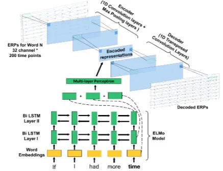
Figure 1: An instance of our framework using a bidi-rectional language model as the text encoder.
2005) profiles. This means that the definition of a component strongly affects interpretation.
There are two typical approaches to resolving these issues. The first is to plot the data and use vi-sual inspection to select an analysis plan, introduc-ing uncontrollable researcher degrees of freedom (Gelman and Loken,2014). Another approach is to run separate models for each time point (or even each electrode) to look for the emergence of an ef-fect. This necessitates complex statistical tests to monitor for inflated Type I error (see, e.g., Blair and Karniski,1993;Laszlo and Federmeier,2014, for discussion) and to control for autocorrelation across time points (Smith and Kutas,2015a,b).
under an autoencoding objective. The decoder CNN can then be decoupled from its encoder and recoupled with any language processing model, thus enabling explicit quantitative comparison of such models. We demonstrate the efficacy of this framework by using it to compare existing sen-tence processing models based on surprisal and/or static word embeddings with novel models based on contextual word embeddings. We find that surprisal-based models actually outperform con-textual word embeddings on their own, but when combined, the two outperform either model alone.
2 Models
All of the models we present have two compo-nents: (i) a pre-trained CNN for decoding raw EEG measurements time-locked to each word in a sentence; and (ii) a language model from which features can be extracted for each word—e.g. the surprisal of that word given previous words or its contextual word embedding. An example model structure using ELMo embeddings (Peters et al., 2018) is illustrated in Figure1.
Convolutional decoder For all models, we use a convolutional decoder pre-trained as a component of an autoencoder. To reduce researcher degrees of freedom, the decoder architecture is selected from a set of possible architectures by cross-validation of the containing autoencoder.
The autoencoder consists of two parts: (a) a convolutional encoder that finds a way to best compress the ERP signals; and (b) a convolutional decoder with a homomorphic architecture that re-constructs the ERP data from the compressed rep-resentation. ERPs were organized into a 2D ma-trix (channel × time points). For the encoder, we pass the ERPs through multiple interleaved 1D convolutional and max pooling layers with re-ceptive fields along the time dimension, shrinking the number of latent channels at each step. Cor-respondingly, for the decoder part, we use a ho-momorphic series of 1D transposed convolutional layers to reconstruct the ERP data.
At train time, the decoder weights are frozen, and the encoder is replaced by one of the language models described below. This entails fitting an in-terface mapping—a linear transformation for each channel produced by the encoder—from the fea-tures extracted from the language model into the representation space output by the encoder.
Language models We consider a variety of fea-tures that can be extracted from a language model.
Surprisal We use the lexical surprisal
−logp(wi |w1, . . . , wi−1)obtained from a RNN
trained byFrank et al.(2015).
Semantic distance Following Frank and Willems(2017), we point-wise average the GloVe embedding (Pennington et al.,2014) of each word prior to a particular word to obtain a context embedding and then calculate the cosine distance between the context embedding and the word
embedding for that word. We use the GloVe
embeddings trained on Wikipedia 2014 and Gigaword 5 (6B tokens, 400K vocabulary size).
Static word embeddings We also consider the GloVe embedding dimensions as features. We do not tune the GloVe embeddings using an ad-ditional recurrent neural network (RNN), instead just passing the them through a multi-layer percep-tron with one hidden layer of tanh nonlinearities. The idea here is that the GloVe-only model tells us how much the distributional properties of a word, outside of the current context, contribute to ERPs.
Contextual word embeddings We consider contextual word embeddings generated from ELMo (Peters et al.,2018) using theallennlp package (Gardner et al.,2017). ELMo produces contextual word embeddings using a combination of character-level CNNs and bidirectional RNNs trained against a language modeling objective, and thus it is a useful contrast to GloVe, since it cap-tures not only a word’s distributional properties, but how they interact with the current context.
We take all three layers of the hidden layer out-put in the ELMo model and concatenate them. To ensure a fair comparison with the surprisal- and GloVe-based models, we use the same tuning pro-cedure employed for the static word embeddings. Further, because sentences are presented incre-mentally in ERP experiments and because ELMo is bidirectional and thus later words in the sen-tence will affect the word embeddings of previous words, we do not obtain an embedding for a par-ticular word on the basis of the entire sentence, in-stead using only the portion of the sentence up to and including that word to obtain its embedding.
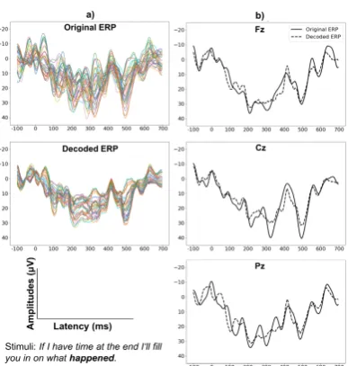
se-Figure 2: Original ERPs and ERPs decoded from the trained autoencoder of an example trial. a) ERPs from all 32 channels (denoted by color). b) Original (solid) and decoded ERPs (dashed) for example electrodes.
mantic distance. The latter features were concate-nated onto the tuned word embeddings before be-ing passed to the interface mappbe-ing.
3 Experiments
We use the EEG recordings collected and modeled by Frank and Willems(2017). In their study, 24 subjects read sentences drawn from natural text. Sentences were presented word-by-word using a rapid serial visual presentation paradigm. We use the ERPs of each word epoched from -100 to 700ms and time-locked to word onset from all the 32 recorded scalp channels. After artifact rejection (provided by Frank and Willems with the data), this dataset contains 41,009 training instances.
Pre-training To select which decoder to use, we compare the performance of two CNN architec-tures motivated by well-known properties of EEG. The first architecture has 5 latent channels and9 time steps. Given the sampling rate and size of the input (250Hz, 200 time steps), this roughly corresponds to filtering the EEG data with alpha band frequency (∼ 10Hz). The other has 10 la-tent channels and20time steps, thus lying within the range of beta band activity (∼ 25Hz). In ad-dition to these two architectures, we also examine whether including subject- and electrode-specific random intercepts improves model performance.
We conduct a 5-fold cross-validation for each architecture to find the one that has the best per-formance in reconstructing ERP data. As shown in Table1, the beta models perform better overall
than alpha models, since they likely capture both alpha and beta band activities. Adding subject-specific intercept, on the other hand, did not greatly improve the model performance.
Model No Intercept Intercept
alpha 49.9 (0.532) 49.7 (0.533)
[image:3.595.84.278.60.264.2]beta 33.5 (0.686) 32.7 (0.692)
Table 1: Mean MSE andR2(in parentheses).
Figure2shows the reconstructed ERPs of the beta model on one trial. The autoencoder can recon-struct the ERP signal very well. The selected channels are illustrative of the reconstruction ac-curacy across all channels. We thus selected the beta model without subject-specific intercept as the decoder for our consequent models.
Training The interface mapping and (where ap-plicable) word embedding tuner are trained un-der an MSE loss using mini-batch gradient de-scent (batch size = 128) with the Adam optimizer (learning rate=0.001and default settings forbeta1,beta2, andepsilon) implemented inpytorch(Paszke et al.,2017). Each model is trained for 200 epochs. Since we need at least one preceding word to compute contextual word em-beddings, we do not include the first word of the sentence. This left ERPs for 1,618 word tokens per subject (638 word types). After excluding tri-als containing artifacts, a total of 37,112 training instances remain.
Development To avoid overfitting, we use early stopping and report the models with the best per-formance on the development set. We did a pa-rameter search over three different weight decays: 1e-5, 1e-3, 1e-1. For each model, we chose the weight decay that produced the best mean performance on held-out data in a 5-fold cross-validation.
Baselines As a baseline we train an intercept-only model that passes a constant input (optimized to best predict the data) to the decoder. In addi-tion, we fit a baseline model that only has word frequency as a feature. Frequency is also included as an additional feature in all models.
Metrics To account for the fact that our model performance is bounded by the performance of the autoencoder, we report a modified form of R2 to evaluate the overall model performance.
R2mod= 1− MSEmodel−MSEautoencoder
[image:3.595.325.503.127.172.2]Model R2
mod 95% CI
Frequency 19.5 [18.5,20.7]
F + Surp 37.4 [36.5,38.3]
F + SemDis 36.1 [32.3,38.4]
F + GLoVE 35.0 [31.8,38.2]
F + ELMo 35.2 [34.3,36.2]
F + S + SD 46.6 [43.5,49.7]
F + S + SD + GloVe 47.1 [43.2,49.4]
[image:4.595.83.280.61.190.2]F + S + SD + ELMo 49.5 [48.9,50.1]
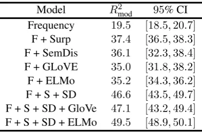
Table 2: Proportion variance explained by each model (×100) and confidence interval across folds computed by a nonparametric bootstrap. F = frequency, S(urp) = surprisal, S(em)D(is) = semantic distance.
4 Results
Table2shows theR2modmetric for each model. We see that both surprisal and semantic distance out-perform both types of word embedding features, all of which outperform frequency alone. When combined, surprisal and semantic distance outper-form either alone, and further gains can be made with the addition of either static (GloVe) or con-textual (ELMo) embedding features. The addition of contextual embedding features increases perfor-mance more than the addition of static word em-bedding features, such that there is some benefit to capturing context over and above that provided by surprisal and semantic distance.
Time course analysis To understand where in time each predictor improved model performance, we examine the increase in correlation over the in-tercept model at each time point (Figure3). There are roughly three regions where the language mod-els outperform the intercept model. The first is right after 100ms post word onset: correspond-ing to the N1 component, which is typically con-sidered to reflect perceptual processing; the sec-ond is between 200 and 350ms: correspsec-onding to the N250 component, which correlates with lexi-cal access (Grainger et al.,2006;Laszlo and Fe-dermeier, 2014); and the third is between 300ms and 500ms: corresponding to the N400, which is typically associated with semantic processing.
[image:4.595.307.527.62.186.2]Consistent with previous findings (Hauk et al., 2006; Laszlo and Federmeier, 2014; Yan and Jaeger, 2019), adding frequency into the model improved model performance in all three time windows. Also consistent with the literature, adding surprisal and semantic distance improved model performance in the N400 time window
Figure 3: Increase in Pearson’s R between predicted and actual ERPs. Lines show GAM smooth over time.
(Frank and Willems,2017;Yan and Jaeger,2019). Models with word embeddings do not differ much from the models containing only frequency, surprisal, and semantic distance, with the biggest difference around 300ms post word onset. This might indicate an effect in the early N400 time window. This could also indicate that processes commonly associated with the N250 may be bet-ter captured by the models containing word em-beddings. If so, it is less expected and potentially interesting, since most of our models have no ac-cess to perceptual properties of the input—with the possible exception of ELMo, whose charCNN may capture orthographic regularities. These ef-fects could reflect our models’ ability to capture top-down lexical processing (see, e.g., Penolazzi et al.,2007;Yan and Jaeger,2019) or possibly sys-tematic correlations between higher-level features and perceptual features.
Predictor βˆ t
Intercept −0.0013 −0.225
Word Type (Content) 0.0030 2.01 ∗
Frequency 0.0110 21.2 ∗∗
Surprisal 0.0050 13.0 ∗∗
Semantic Distance 0.0040 11.60 ∗∗
GloVe Embeddings 0.0040 10.3 ∗∗
ELMo Embeddings 0.0040 10.1 ∗∗
Freq : Word Type −0.0010 −2.43 ∗
Surp : Word Type 0.0001 0.24
SemDis : Word Type −0.0003 −0.70
GloVe : Word Type 0.0002 0.55
[image:5.595.72.292.63.245.2]ELMo : Word Type 0.0007 −1.85 +
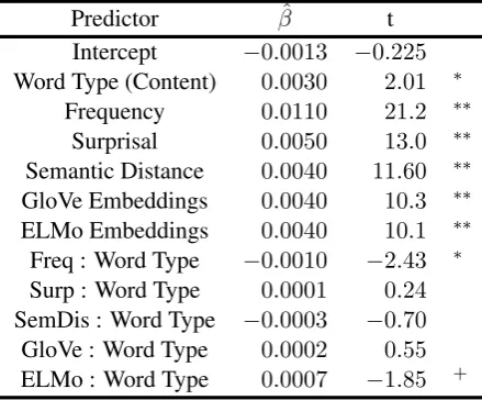
Table 3: Model estimates and t statistics from mixed-effects model.∗∗:p <0.01;∗:p <0.05;+ :p <0.1
types (function=-1, content=1).
Table3shows the resulting coefficients. Over-all, models display better performance for content words than for function words (βˆ = 0.003, t = 2.01,p < 0.05), consistent with previous find-ings (Frank et al., 2015). Including each type of information also significantly increased model fit (ts > 10.1,p < 0.01). There was a signifi-cant interaction between frequency and word type (βˆ = −0.001, t = −2.43,p < 0.02): including frequency increased model performance for func-tion words more than for content words. There was also a marginally significant interaction be-tween ELMo and word type (βˆ = 0.0007, t =
−1.85,p < 0.064), suggesting that including ELMo embeddings increased model performance for content words more than for function words.
We also examine the interaction between each type of information and each part-of-speech. Overall, the models had worse performance for particles (βˆ = −0.017, t = −3.37,p < 0.01), nouns (βˆ = −0.007, t = −1.95,p < 0.051) and pronouns (βˆ = −0.012, t = −1.76,p < 0.08). Including each type of information increased over-all model fit (ts > 6.05,p < 0.01). While including frequency increased overall model fit, it increased the model fit for verbs less (βˆ =
−0.003, t = −2.04,p < 0.05). No other effects reached significance.
5 Related Work
Traditionally, ERP studies of language process-ing use coarse-grained predictors like cloze rates, which often lack the precision to differentiate dif-ferent neural computational models (for
discus-sion, seeYan et al.,2017;Rabovsky et al.,2018). To overcome such limitations, a main line of attack has been to extract measures from probabilistic language models and evaluate them against ERP amplitudes (Frank et al., 2015; Brouwer et al., 2017;Rabovsky et al.,2018;Delaney-Busch et al., 2019;Fitz and Chang,2018;Szewczyk and Wod-niecka,2018;Biemann et al.,2015).
While prior studies have also predicted ERPs from language model-based features (Broderick et al.,2018;Frank and Willems,2017;Hale et al., 2018), they fit to aspects of the EEG signals that are unlikely to be related to language processing. Our approach threads the needle by first finding abstract structure in the ERPs with a CNN, then using that knowledge in predicting that structure from linguistic features. We are not the first to use CNNs to model EEG/ERPs (Lawhern et al.,2016; Schirrmeister et al., 2017; Seeliger et al., 2018; Acharya et al., 2018; Moon et al., 2018), but to our knowledge, no other work has yet used CNNs for modeling ERPs during reading.
6 Conclusion
We proposed a novel framework for modeling ERPs collected during reading. Using this frame-work, we compared the abilities of a variety of existing and novel sentence processing models to reconstruct ERPs, finding that modern contextual word embeddings underperform surprisal-based models but that, combined, the two outperform ei-ther on its own.
ERP data provides a rich testbed not only for comparing models of language processing, but po-tentially also for probing and improving the rep-resentations constructed by natural language pro-cessing (NLP) systems. We provided one example of how such probing might be carried out by ana-lyzing the differences among models as a function of processing time, but this analysis only scratches the surface of what is possible using our frame-work, especially for understanding the more com-plex neural models used in NLP.
Acknowledgments
References
U Rajendra Acharya, Shu Lih Oh, Yuki Hagiwara, Jen Hong Tan, and Hojjat Adeli. 2018. Deep convo-lutional neural network for the automated detection and diagnosis of seizure using EEG signals. Com-puters in biology and medicine, 100:270–278.
Stanislaw Antol, Aishwarya Agrawal, Jiasen Lu, Mar-garet Mitchell, Dhruv Batra, C Lawrence Zitnick, and Devi Parikh. 2015. VQA: Visual Question An-swering. In Proceedings of the IEEE international
conference on computer vision, pages 2425–2433.
Chris Biemann, Steffen Remus, and Markus J Hof-mann. 2015. Predicting word ‘predictability’ in cloze completion, electroencephalographic and eye movement data. InProceedings of natural language processing and cognitive science, pages 83–93. Li-breria Editrice Cafoscarina.
R Clifford Blair and Walt Karniski. 1993. An alterna-tive method for significance testing of waveform dif-ference potentials. Psychophysiology, 30(5):518– 524.
Michael P Broderick, Andrew J Anderson, Giovanni M Di Liberto, Michael J Crosse, and Edmund C Lalor. 2018. Electrophysiological correlates of semantic dissimilarity reflect the comprehension of natural, narrative speech.Current Biology, 28(5):803–809.
Harm Brouwer, Matthew W Crocker, Noortje J Ven-huizen, and John CJ Hoeks. 2017. A neurocompu-tational model of the N400 and the P600 in language processing.Cognitive Science, 41:1318–1352.
Michael Dambacher, Reinhold Kliegl, Markus Hof-mann, and Arthur M Jacobs. 2006. Frequency and predictability effects on event-related potentials dur-ing readdur-ing. Brain Research, 1084(1):89–103.
Nathaniel Delaney-Busch, Emily Morgan, Ellen Lau, and Gina R Kuperberg. 2019. Neural evidence for bayesian trial-by-trial adaptation on the N400 during semantic priming. Cognition, 187:10–20.
Katherine A DeLong, Thomas P Urbach, and Marta Kutas. 2005. Probabilistic word pre-activation dur-ing language comprehension inferred from electri-cal brain activity. Nature Neuroscience, 8(8):1117– 1121.
Hartmut Fitz and Franklin Chang. 2018. Sentence-level erp effects as error propagation: A neurocom-putational model.PsyArXiv.
Stefan L Frank, Leun J Otten, Giulia Galli, and Gabriella Vigliocco. 2015. The ERP response to the amount of information conveyed by words in sen-tences. Brain and Language, 140:1–11.
Stefan L Frank and Roel M Willems. 2017. Word predictability and semantic similarity show distinct patterns of brain activity during language compre-hension. Language, Cognition and Neuroscience, 32(9):1192–1203.
Matt Gardner, Joel Grus, Mark Neumann, Oyvind Tafjord, Pradeep Dasigi, Nelson F. Liu, Matthew Peters, Michael Schmitz, and Luke S. Zettlemoyer. 2017. AllenNLP: A Deep Semantic Natural Lan-guage Processing Platform.
Andrew Gelman and Eric Loken. 2014. The statistical crisis in science. The best writing on mathematics, 102(6):460–465.
Jonathan Grainger, Kristi Kiyonaga, and Phillip J Hol-comb. 2006. The time course of orthographic and phonological code activation. Psychological Sci-ence, 17(12):1021–1026.
Peter Hagoort, Lea Hald, Marcel Bastiaansen, and Karl Magnus Petersson. 2004. Integration of word meaning and world knowledge in language compre-hension. Science, 304(5669):438–441.
John Hale, Chris Dyer, Adhiguna Kuncoro, and Jonathan Brennan. 2018. Finding syntax in human encephalography with beam search. In Proceed-ings of the 56th Annual Meeting of the Association for Computational Linguistics (Volume 1: Long
Pa-pers), pages 2727–2736. Association for
Computa-tional Linguistics.
Olaf Hauk, Matthew H Davis, M Ford, Friedemann Pulverm¨uller, and William D Marslen-Wilson. 2006. The time course of visual word recognition as re-vealed by linear regression analysis of ERP data.
Neuroimage, 30(4):1383–1400.
MD. Zakir Hossain, Ferdous Sohel, Mohd Fairuz Shi-ratuddin, and Hamid Laga. 2019. A comprehen-sive survey of Deep Learning for Image Captioning.
ACM Comput. Surv., 51(6):118:1–118:36.
Albert Kim and Lee Osterhout. 2005. The indepen-dence of combinatory semantic processing: Evi-dence from event-related potentials. Journal of
Memory and Language, 52(2):205–225.
Gina R Kuperberg. 2016. Separate streams or proba-bilistic inference? what the N400 can tell us about the comprehension of events. Language, Cognition
and Neuroscience, 31(5):602–616.
Gina R Kuperberg, Tatiana Sitnikova, David Caplan, and Phillip J Holcomb. 2003. Electrophysiological distinctions in processing conceptual relationships within simple sentences. Cognitive Brain Research, 17(1):117–129.
Marta Kutas and Steven A Hillyard. 1980. Reading senseless sentences: Brain potentials reflect seman-tic incongruity. Science, 207(4427):203–205.
Sarah Laszlo and Kara D Federmeier. 2014. Never seem to find the time: evaluating the physiological time course of visual word recognition with regres-sion analysis of single-item event-related potentials.
Language, Cognition and Neuroscience, 29(5):642–
Ellen F Lau, Colin Phillips, and David Poeppel. 2008. A cortical network for semantics:(de) con-structing the N400. Nature Reviews Neuroscience, 9(12):920–933.
Vernon J Lawhern, Amelia J Solon, Nicholas R Way-towich, Stephen M Gordon, Chou P Hung, and Brent J Lance. 2016. EEGnet: A compact convo-lutional network for EEG-based bracomputer in-terfaces. arXiv preprint arXiv:1611.08024.
Seong-Eun Moon, Soobeom Jang, and Jong-Seok Lee. 2018. Convolutional neural network approach for EEG-based emotion recognition using brain connec-tivity and its spatial information. In 2018 IEEE International Conference on Acoustics, Speech and
Signal Processing (ICASSP), pages 2556–2560.
IEEE.
Anna C Nobre and Gregory McCarthy. 1994. Language-related erps: Scalp distributions and mod-ulation by word type and semantic priming.Journal of Cognitive Neuroscience, 6(3):233–255.
Lee Osterhout and Phillip J Holcomb. 1992. Event-related brain potentials elicited by syntactic anomaly. Journal of Memory and Language, 31(6):785–806.
Adam Paszke, Sam Gross, Soumith Chintala, Gre-gory Chanan, Edward Yang, Zachary DeVito, Zem-ing Lin, Alban Desmaison, Luca Antiga, and Adam Lerer. 2017. Automatic differentiation in pytorch.
Jeffrey Pennington, Richard Socher, and Christopher Manning. 2014. Glove: Global vectors for word representation. InProceedings of the 2014 confer-ence on empirical methods in natural language
pro-cessing (EMNLP), pages 1532–1543.
Barbara Penolazzi, Olaf Hauk, and Friedemann Pul-verm¨uller. 2007. Early semantic context integration and lexical access as revealed by event-related brain potentials. Biological Psychology, 74(3):374–388.
Matthew Peters, Mark Neumann, Mohit Iyyer, Matt Gardner, Christopher Clark, Kenton Lee, and Luke Zettlemoyer. 2018. Deep contextualized word repre-sentations. InProceedings of the 2018 Conference of the North American Chapter of the Association for Computational Linguistics: Human Language
Technologies, Volume 1 (Long Papers), volume 1,
pages 2227–2237.
Milena Rabovsky, Steven S Hansen, and James L Mc-Clelland. 2018. Modelling the N400 brain potential as change in a probabilistic representation of
mean-ing. Nature Human Behaviour, 2(9):693–705.
Robin Tibor Schirrmeister, Jost Tobias Springenberg, Lukas Dominique Josef Fiederer, Martin Glasstet-ter, Katharina Eggensperger, Michael Tangermann, Frank Hutter, Wolfram Burgard, and Tonio Ball. 2017. Deep learning with convolutional neural net-works for EEG decoding and visualization. Human
Brain Mapping, 38(11):5391–5420.
Katja Seeliger, Matthias Fritsche, Umut G¨uc¸l¨u, Sanne Schoenmakers, Jan-Mathijs Schoffelen, Sander Bosch, and Marcel van Gerven. 2018. Convolu-tional neural network-based encoding and decoding of visual object recognition in space and time.
Neu-roImage, 180:253–266.
Sara C Sereno, Keith Rayner, and Michael I Posner. 1998. Establishing a time-line of word recognition: evidence from eye movements and event-related po-tentials. Neuroreport, 9(10):2195–2200.
Nathaniel J Smith and Marta Kutas. 2015a. Regression-based estimation of ERP wave-forms: I. the rERP framework. Psychophysiology, 52(2):157–168.
Nathaniel J Smith and Marta Kutas. 2015b. Regression-based estimation of ERP waveforms: Ii. nonlinear effects, overlap correction, and practical considerations. Psychophysiology, 52(2):169–181.
Jakub M Szewczyk and Zofia Wodniecka. 2018. The mechanisms of prediction updating that impact pro-cessing of upcoming words – an event-related study on sentence comprehension. PsyArXiv.
Cyma Van Petten and Barbara J Luka. 2012. Pre-diction during language comprehension: Benefits, costs, and ERP components. International Journal of Psychophysiology, 83(2):176–190.
Shaorong Yan and T. Florian Jaeger. 2019. (Early) context effects on event-related potentials over natu-ral inputs. Language, Cognition and Neuroscience, pages 1–22.