Modelling multi modal sound transmission from point sources in ducts with flow using a wave based method

FROM POINT SOURCES IN DUCTS WITH FLOW USING

A WAVE-BASED METHOD

Gareth J. Bennett, Ciar´an J. O’Reilly, Hao Liu

Dept. of Mechanical and Manufacturing Engineering, Trinity College, Dublin 2, Ireland. email: [email protected]

Ulf Tapken

German Aerospace Center (DLR),

Institute of Propulsion Technology, Engine Acoustics Branch, Muller-Breslau-Str. 8, 10623 Berlin, Germany.

An understanding of the multi-modal propagation of acoustic waves in ducts is of practical interest for use in the control of noise in, for example, aero-engines, automotive exhaust and ventilation systems. In this paper, the propagation of sound from point sources in hard-walled ducts is modelled using a numerical wave-based approach, referred to as the wave expansion method. This is a highly efficient full-domain discretisation method, which requires as few as two-to-three mesh points per wavelength. An inhomogeneous potential flow may be easily included in the method. The numerical solution for point sources embedded in the wall of a circular duct with non-reflective end-conditions and a uniform axial flow is compared with an analytical Green’s function solution. A modal decomposition technique is used to provide de-tailed information about the modal content of the sound field. This study provides an insightful comparison between an analytical and numerical solution to the acoustic field in a duct. The accuracy and robustness of the wave expansion method is assessed for this benchmark problem before its versatility is demonstrated with examples.

1.

Introduction

2.

Description of Mode Propagation in Hard Walled Cylindrical Flow

Ducts

For acoustic propagation in an infinite hard walled cylindrical duct with superimposed constant

mean flow velocity U, the pressurep=p(r, θ, x, t), in cylindrical coordinates, is found as a solution

of the homogeneous convective wave equation,

1

c2

D2_p

Dt2 −

∂2_p

∂x2 −

1 r ∂ ∂r r∂p ∂r − 1 r2

∂2_p

∂θ2 = 0 (1)

where the substantive derivative is defined to be

D

Dt =

∂

∂t +U.∇

This solution is found as a combination of the characteristic functions of equation (1) each of which satisfy specific boundary conditions. Rigorous treatments of the derivation of the separation-of-variables solution can be found in the literature [3, 4, 5] . For the following assumptions that;

• The flow is incompressible and isentropic with negligible temperature gradients

• The mean flow speed, U= (Ux,0,0)is stationary with time

• The axial mean flow profile as well as the duct cross-sectional area are invariant in the axial

direction

• The mean temperature and the density are stationary in space and time

the solution to the wave equation for the complex pressure can be given by a linear superposition of modal terms:

ˆ

p(x, r, ϕ) =

∞

X

m=−∞ ∞

X

n=0

h A+m,ne(

−_jk+_m,nx)

+A−m,ne(+

jk−m,nx)

i

fm,n(r)e(jmϕ) (2)

whereA+

m,n andA

−

m,n are the complex amplitudes of the modes,k+m,nxandk

−

m,nxare the axial wave

numbers, and m and n are the azimuthal and radial mode indices respectively. The + superscript

refers to the direction of flow whereas the−superscript indicates the parameter to be defined counter

to the flow direction. In the case of hard-walled acoustic boundary conditions, the modes form an orthogonal eigensystem, with a modal shape factor given by

fm,n(r) =

Jm(σmnr/R)

p Nm,n

(3)

for a non-annular cylinder. In equation (3), Jm is a Bessel function of the first kind of orderm with

associated hard-walled cylindrical eigenvalueσmn. R is the duct outer radius and in order to satisfy

orthogonality the normalisation factor is calculated to be

Nmn = 2π

Z R

0

J2_m(σmnr/R)r dr =πR2 J2m(σmn)−Jm−₁(σ_mn)J_m+1(σ_mn)

(4)

The normalisation transforms the orthogonal mode eigensystem into an orthonormal mode eigensys-tem. A mean flow can be accommodated in the formulation by modification of the axial wave numbers

which are a function of the mode eigenvalueσmnand the free field propagation wave number, k, which

are defined as follows

k±

mn =k

−Mx±αmn

β2 where αmn =

s 1− βσmn kR 2

and β =p1−M2

3.

Wave Expansion Method

If the mean flow is assumed to be irrotational and inhomogeneous then it can be modelled as a

potential flow, and the governing field equation for the velocity potential,φis given by

1

ρ∇.(ρ∇φ)−L

1

c2Lφ

= 0 (6)

whereLis the complex linear operator(iω+U.∇)andU,ρ,c, are the local mean velocity, density,

and speed of sound respectively. The acoustic parts of the velocity potential and pressure are related by

ˆ

p=−ρjωφ−ρU.∇φ (7)

The velocity potential at a discrete point,φ0, (the subscript ‘0’ denotes the value at the point in

question) may be computed from the amplitude and phase of M neighbouring points. The potential

at each point in a domain may be approximated by the superposition of the field generated by N

hypothetical plane waves of strengthγnand with unit propagation in directiondnsuch that

φ0 =

N

X

n=1

γnexp [−iq(d.x0)] = hγ (8)

wherehn = exp [−iq(d.x0)],

q = iB0.d±

q

4K2

0 1−(M0.d)

2

−(B0.d)2

2 1−(M0.d)2 (9)

where

B= 2ikM+U.∇

1

c2

U+ 1

c2U.∇U−

1

ρ∇ρ (10)

K2 ₌ ω2

c2 −iωU.∇

1

c2 (11)

and whereM = U/c. Similarly, the velocity potential at a neighbouring point,m, in the

computa-tional lattice, wherem= 1,2, .., M, is given as

φm =

N

X

n=1

γnexp [−iq(d.xm)] = Hγ (12)

IfH+is the pseudo-inverse ofHthen

γ=H+φm, (13)

and substituting this back into equation (8) leads to

φ0−hH+φm = 0. (14)

If the he local stiffness vector for a computational lattice isκ0 =−hH+, then

which may be rewritten as

1 κ0

φ0

φm

= 0. (16)

For the total computational domain, with a source vector,f, added to the right-hand-side and where

κis the overall stiffness matrix, a linear system of equations may be defined of the form

κφ=f. (17)

This may, with the addition of appropriate boundary conditions (see [6]), be solved for φ, a vector

containing the velocity potential at each point in the overall computational lattice.

4.

Analytical Solution in Terms of Point Source Distribution

In order to have a benchmark case against which the Wave Based Method could be compared, results from an exact analytical solution were generated. The frequency-domain Green’s function for a duct with an axial irrotational mean flow must satisfy

∇2−Mx2

∂2

∂x2 −2ikMx

∂ ∂x +k

2

G(x,y) =−δ(x−y) (18)

and for a hard-walled boundary condition

∂G

∂n = 0 (19)

where n is a unit vector normal to the surface of the duct.

Following the formulation of Goldstein [7], the sound pressure generated at position (x, r, ϕ)

due to a single monopole source with volume velocity q0 = v0A located at (xq0, rq0, ϕq0) can be

expressed as

p(⇆₎

(x, r, ϕ|xq0, rq0, ϕq0) = −jωρq0g(

⇆₎

(x, r, ϕ|xq0, rq0, ϕq0) (20)

=q0

ρc

2

∞

X

m=−∞ ∞

X

n=0

Jm(σmnr/R)Jm(σmnrq0/R)

αmnNmn

e−im(φ−φq0)e−ik

±

mn(x−xq0)

(21)

whereq0 is the source volume velocity,ρandcare the density and speed of sound of the propagation

medium.

Whereas a single monopole source will excite all modes, specific modes can be excited by locat-ing multiple sources around the duct and by adjustlocat-ing their phases appropriately uslocat-ing the expressions of equation 22. The total sound field is found through superposition of equation 21 for each source.

q(θl) =qme(im

2πl

S ) where

l = 0,1, . . . ,(S−1);

θl =

2πl

S

(22)

5.

Results and Analysis

results for a comparison between the analytical solution and those from the WEM for a Helmholtz number of 5.9. The agreement is seen to be very good both on the wall surface and within the volume of the duct.

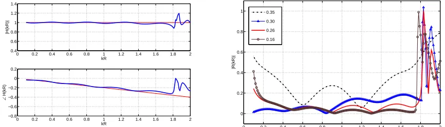
Some investigation of the sensitivity of the results as a function of mesh density for the WEM was carried out, the results of which can be seen in figure 2. The theoretical and numerical results

for the transfer function for a mesh nodal spacing of 0.26m is shown in figure 2(a). Using a two

microphone technique such as that of Chung and Blaser’s [8], the reflection coefficient for the plane wave frequency range can be calculated, results of which are shown in figure 2(b). As can be seen, the results are improved upon by increasing the number of points per wavelength, however, if the density is too great the low frequency results disimprove. This is due to ill-conditioning in the system matrices. Thus, an optimum density must be employed for the frequency range of interest.

The next comparison was performed with eight monopole sources to excite a specific azimuthal

mode, in this caseAm =A1. Figures 3 and 4 show the comparison between the pressure fields for two

Helmholtz numbers, the higher one being above the cut-on frequency of the first radial mode. Again

the comparison is excellent although being180degrees out of phase with each other presumably due

to a phase shift in the monopole phases between the two cases.

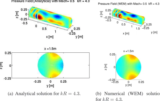
The model’s capability to incorporate a mean flow is demonstrated in figure 5. In both cases, which agree closely, the wavelengths are modified upstream and downstream of the monopole source.

5.1 Acoustic Modal Decomposition in Hard Walled Cylindrical Flow Ducts

The gain some deeper insight into the pressure field comparisons, a modal decomposition was performed using both sets of data. The method employed in this paper is based on the approach

proposed by ˚Abom [9] and further details can be found in Bennett [10, 11], where this technique

was implemented with both experimental and numerical data. Similar to the techniques described by Enghardt et al. [12] and Tapken and Enghardt [13], the procedure uses an array of axially and azimuthally distributed wall surface location measurements, and consists of solving equation (2) for

the modal amplitudes,A±

m,n. The configuration for the “microphone” arrays are four axial locations

separated by0.05mof ten sensors equispaced around the circumference of the0.5mdiameter duct.

The results are presented in figure 6. Qualitatively the results agree well for the most part with some minor differences. However, the magnitudes do not agree. Further work will have to be performed to determine the correct monopole volume source magnitude. In addition, although not plotted, the reflected radial modes from the WEM data, are in some instances very large, in contrast to the modes decomposed from the analytical data which are correctly close to zero for the infinite duct case. It is thought that the reason for this is that the radiation condition which was inherited from a free field configuration is inappropriate for the duct.

5.2 Versatility of the Wave Expansion Method.

Figure 7 shows a simple example of how the WEM method may be used to study a complex duct shape. Although the results are not verified here, qualitatively they appear to be correct with the higher modes clearly seen to be cut-off leaving only plane wave modes when the Helmholtz number

is reduced to belowkR= 1.83in figure 7(b).

A second interesting result is seen in figure 8, where theAm =A3mode is excited below its

6.

Conclusions

In this paper, the propagation of sound from point sources in hard-walled ducts is modelled using a numerical wave-based approach, referred to as the wave expansion method. The results are compared to an analytical Green’s function solution. The pressure fields are found to compare extremely well when either specific or all acoustic modes are excited. The numerical solution is found to be sensitive to the mesh density with diminishing returns to be gained with increasing density. An acoustic modal decomposition was performed on the data, in both cases, with good qualitative agreement found for the azimuthal and incident radial modes. However, the reflected modes are erroneously high. This is thought to be due to a badly defined radiation condition at the end of the duct. Also, the monopole source magnitudes will have to be more correctly calculated to improve the agreement in the modal magnitudes. The versatility of the numerical (WEM) solution is demonstrated by examining a duct geometry of varying duct diameter and by its ability to study evanescent waves.

(a) Analytical solution forkR= 5.9. (b) Numerical (WEM) solution for kR = 5.9.

Figure 1. Pressure field in a duct excited by a single monopole source located on the duct surface at

(x, y, z) = (0,−0.25,0)

0 0.2 0.4 0.6 0.8 1 1.2 1.4 1.6 1.8 2 0.4

0.6 0.8 1 1.2 1.4

kR

|H(kR)|

0 0.2 0.4 0.6 0.8 1 1.2 1.4 1.6 1.8 2 −0.8

−0.6 −0.4 −0.2 0 0.2

kR

∠

H(kR)

(a) Transfer function between two points on duct at same azimuthal angle separated axially by0.05m. The-ory versus numerical results with mesh density of

0.26m.

0 0.2 0.4 0.6 0.8 1 1.2 1.4 1.6 1.8 2 0

0.2 0.4 0.6 0.8 1

kR

|R(kR)|

0.35 0.30 0.26 0.16

(b) Reflection coefficient as a function of mesh density.

(a) Analytical solution for kR= 2.5.

(b) Numerical solution (WEM) forkR= 2.5.

Figure 3. Pressure field in a duct excited by eight monopole sources located equidistant around the duct surface atx= 0. Phases of monopoles adjusted to exciteAm=A1.

(a) Analytical solution for kR = 5.9.

(b) Numerical solution (WEM) forkR= 5.9.

Figure 4. Pressure field in a duct excited by eight monopole sources located equidistant around the duct surface atx= 0. Phases of monopoles adjusted to exciteAm=A1.

(a) Analytical solution forkR= 4.3. (b) Numerical (WEM) solution forkR= 4.3.

Figure 5. Pressure field in a duct excited by a single monopole source located on the duct surface at

0 1 2 3 4 5 6 0 20 40 60 |Aplus(kR)|

Azimuthal Modes Decomposition (Incident)

0 1 2 3 4 5 6

0 20 40 60

|Aplus(kR)|

Radial Modes Decomposition (Incident)

kR Modes 0

Modes ±1 Modes ±2 Modes±3 Modes ±4

(0,0) ( ±1,0) ( ±2,0) (±3,0) (±4,0) (±1,1) ( 0,1)

(a) Modal decomposition using analytical data.

0 1 2 3 4 5 6

0 0.5 1 1.5

|Aplus(kR)|

Azimuthal Modes Decomposition (Incident)

0 1 2 3 4 5 6

0 0.5 1 1.5 kR |Aplus(kR)|

Radial Modes Decomposition (Incident) (0,0)

( ±1,0) ( ±2,0) (±3,0) (±4,0) (±1,1) ( 0,1) Modes 0 Modes ±1 Modes ±2 Modes±3 Modes ±4

(b) Modal decomposition using numerical (WEM) data.

Figure 6. Azimuthal and radial (incident) modal decomposition in the duct excited by a monopole source.

−0.5 0 0.5 1 1.5 2 2.5 −0.10 0.1 −0.1 0 0.1 y [m] x [m]

WEM Sound Field kR = 4.1

z [m]

(a)kR= 4.1for larger diameter reducing tokR= 2.05

for the smaller diameter.

−0.5 0 0.5 1 1.5 2 2.5 −0.10 0.1 −0.1 0 0.1 y [m] x [m]

WEM Sound Field kR = 3.2

z [m]

(b) kR= 3.2for larger diameter reducing tokR= 1.6

for the smaller diameter.

Figure 7. Pressure field in a cylindrical duct of non-constant diameter, excited by a single monopole source. Numerical (WEM) solution.

−0.5 0

0.5 1

1.5 −0.250 0.25 −0.25 0 0.25 y [m] x [m] z [m]

−0.25 0 0.25 −0.25

0 0.25

x =0.00m

z [m]

−0.25 0 0.25 −0.25 0 0.25 y [m] x =0.25m z [m]

−0.25 0 0.25 −0.25 0 0.25 y [m] x =1.5m z [m]

REFERENCES

1 _{J. E. Caruthers, R. C. Engels, and G. K. Ravinprakash. A wave expansion computational method}

for discrete frequency acoustics within inhomogeneous flows. In AIAA/CEAS 2nd Aeroacoustics

Conference, State College, Pennsylvania, USA, 1996. AIAA-1996-1684.

2 _{L. Barrera Rolla and H.J. Rice. A forward-advancing wave expansion method for numerical}

so-lution of large-scale sound propagation problems. Journal of Sound and Vibration, 296(1-2):406– 415, 2006.

3 _{P. Mungur and G. M. L. Gladwell. Acoustic wave propagation in a sheared fluid contained in a}

duct. Journal of Sound and Vibration, 9:28–48, 1969.

4 _{M. L. Munjal. Acoustics of Ducts and Mufflers. John Wiley and Sons, 1987.}

5 _{L. E. Kinsler, A. R. Frey, A. B. Coppens, and J. V. Sanders. Fundamentals of Acoustics. John}

Wiley and Sons, fourth edition, 2000.

6 _{G. Ruiz. Numerical vibro/acoustic analysis at higher frequencies. PhD thesis, University of}

Dublin, Trinity College, 2002.

7 _{M. E. Goldstein. Aeroacoustics. McGraw-Hill International Book, 1976.}

8 _{J. Y. Chung and D. A. Blaser. Transfer function method of measuring in-duct acoustic properties.}

i. theory. J. Acoust. Soc. Am., 68(3):907–913, 1980.

9 _{Mats ˚Abom. Modal decomposition in ducts based on transfer function measurements between}

mi-crophone pairs. Technical Report Report TRITA-TAK-8702, Department of Technical Acoustics, Royal Institute of Technology, Stockholm, Sweden, 1987.

10 _{G. J. Bennett. Noise Source Identification For Ducted Fans. PhD thesis, Trinity College Dublin,}

2006.

11 _{Gareth J. Bennett, Ciaran O’Reilly, Ulf Tapken, and John Fitzpatrick. Noise source location in}

turbomachinery using coherence based modal decomposition. In 15th AIAA /CEAS Aeroacoustics

Conference, number AIAA-2009-3367, Miami, Florida, May 11-13 2009.

12 _{Lars Enghardt, Yanchang Zhang, and Wolfgang Neise. Experimental verification of a radial mode}

analysis technique using wall-flush mounted sensors. In 137th Meeting of the Acoustical Society

of America, Berlin, March 1999.

13 _{U. Tapken and L. Enghardt. Optimization of sensor arrays for radial mode analysis in flow ducts.}