YNU HPCC at SemEval 2017 Task 4: Using A Multi Channel CNN LSTM Model for Sentiment Classification

(1)

YNU-HPCC at SemEval 2017 Task 4: Using A Multi-Channel

CNN-LSTM Model for Sentiment Classification

Haowei Zhang, Jin Wang, Jixian Zhang, Xuejie Zhang

School of Information Science and Engineering

Yunnan University

Kunming, P.R. China

Contact: xjzhang@ynu.edu.cn

Abstract

In this paper, we propose a multi-channel convolutional neural network-long short-term memory (CNN-LSTM) model that consists of two parts: multi-channel CNN and LSTM to analyze the sentiments of short English messages from Twitter. Un-like a conventional CNN, the proposed model applies a multi-channel strategy that uses several filters of different length to ex-tract active local n-gram features in differ-ent scales. This information is then sequen-tially composed using LSTM. By combin-ing both CNN and LSTM, we can consider both local information within tweets and long-distance dependency across tweets in the classification process. Officially re-leased results show that our system outper-forms the baseline algorithm.

1 Introduction

Social network services (SNSs) such as Twitter, Fa-cebook, and Weibo are used daily to express thoughts, opinions, and emotions. In Twitter, 6000 short messages (tweets) are posted by users every second1_{. Therefore, Twitter is considered as one of}

the most concentrated opinion-expressing venues on the Internet. Subjective analysis of this type of user-generated content has become a vital task for politics, social networking, marketing, and adver-tising.

The potential application of sentiment analysis has been the motivation behind the SemEval 2017 Task 4, which is a competition involving a series of subtasks that focus on Twitter sentiment classifica-tions. Subtask A involves message polarity classi-fication, which requires a system to classify

1_{http://www.internetlivestats.com/twitter-statistics/}

whether a message is of positive, negative, or neu-tral sentiment. Subtasks B and C involve topic-based message polarity classification, which re-quire a system to classify a message on two- and five-point scales toward a certain topic.

Various approaches have been proposed to ana-lyze sentiment of text, and deep neural network has achieved state-of-the-art results in recent years. Proven successful text classification methods in-clude convolutional neural networks (CNN)

(LeCun et al., 1990; Y. Kim, 2014; Kalchbrenner

et al., 2014) and Long Short-Term Memory

(LSTM) (Hochreiter et al, 1997; Tai et al., 2015). In general, CNN applies a convolutional layer to extract active local n-gram features, but lost the or-der of words. By contrast, LSTM can sequentially model texts. However, it focuses only on past in-formation and draws conclusions from the tail part of texts. It fails to capture the local response from temporal data.

In this paper, we propose a multi-channel CNN-LSTM model for sentiment classification. It con-sists of two parts: multi-channel CNN, and LSTM. Unlike a conventional CNN model, we apply a multi-channel strategy that uses several filters of different length. The model is thus able to extract active n-gram features of different scales. LSTM is then applied to compose those features sequentially. By combining both CNN and LSTM, both local in-formation within tweets and long-distance depend-ency across tweets can be considered in the classi-fication process. To train the proposed neural model effectively using many parameters, we pre-trained the model using a distant supervision ap-proach (Go et al., 2009).In our experiment, we pre-sented our participation of the proposed model for

(2)

the SemEval 2017 Task 4 Subtasks A, B, and C (Rosenthal et al., 2017).

The remainder of this paper is organized as fol-lows. In Section 2, we detail the architecture and multi-channel strategy of our model. Section 3 summarizes the comparative results of our pro-posed model against the baseline algorithm. Sec-tion 4 offers a conclusion.

[image:2.595.91.520.73.346.2]

2 Multi-Channel CNN-LSTM Model

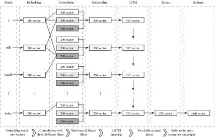
Figure 1 shows the architecture of our model. The model consists of six types of layers: embedding, convolution, max-pooling, LSTM, dense, and soft-max. First, a tweet is input as a series of vectors of constituent words and transformed into a feature matrix by an embedding layer. The feature matrix is then passed into three parallel CNNs having dif-ferent filter lengths. The max pooling layer extracts the max-over different CNNs results that are in-tended to be the salient features, and input them to the LSTM layer. Then, normal dense and softmax layers use outputs from LSTM and output the final classification result.

2.1 Embedding Layer

The embedding layer is the first layer of the model. Each tweet is regarded as a sequence of word to-kens t1, t2, …, tN, where N is the length of the token

vector. According to statistics of tweets collected

from twitter in Section 3.1, about 95% tweets is shorter than 30 words. Thus, we empirically limit the maximum of N to 30. Any tweet longer than 30 tokens is truncated to 30, and any tweet shorter than 30 is padded to 30 using zero padding. Every word is mapped to a d-dimension word vector. The out-put of this layer is a matrix N d

T  .

2.2 CNN Layer

In each CNN layer, m filters are applied to a sliding window of width w over the matrix of previous em-bedding layer. Let w d

F  denote a filter matrix

and b a bias. Assuming that Ti:i+j denotes the token

vectors ti, ti+1, …, ti+j (if k > N, tk= 0), the result of

each filter will be _{, where the}i-th element of f is generated by:

: 1

i i i w

f



T

_{ }

 

F b

(1)

where



denotes convolution action. Before pro-cessing f to the next layer, a nonlinear activation function is applied. Here, we use ReLU function (Nair and Hinton, 2010) for faster calculation. Con-volving filters with window width w can extract w -gram feature. By applying multiple convolving fil-ters in this layer, we can extract active local n-gram features in different scales. To keep output sizes of different filters identical, we apply zero padding to token vectors before convolution.

d

f

Figure 1:Architecture of the proposed CNN-LSTM model.

200 vector

200 vector 200 vector 512 vector

200 vector

200 vector Embedding

Words Convolution Max pooling LSTM Dense Softmax

Embedding words into vectors

Convolution with three di fferent filters

Max-over di fferent filters

LSTM encoding

Two fully connect layers

Softmax to multi catogeries and output I

will

watch

(3)

2.3 Max-over Pooling Layer

In this layer, the maximum value from different fil-ters is taken as the most salient feature. Because the CNN layer with window width w can extract w -gram features, the maximum values of the output from CNN layer are considered the most salient in-formation in the target tweet. We choose max rather than mean pooling because the salient feature rep-resents the most distinguishing trait of a tweet.

2.4 LSTM Layer

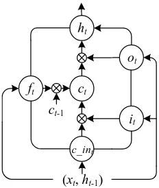
The architecture of a recurrent neural network (RNN) is suitable for processing sequential data. However, a simple RNN is usually difficult to train because of the gradient vanishing problem. To ad-dress this problem, LSTM introduces a gating structure that allows for explicit memory updates and deliveries. As shown in Figure 2, LSTM calcu-lates hidden state ht using the following equations:  Gates:

1

( )

t xi t hi t i

t xf t hf t f

t xo t ho t i

i W x W h b f W x W h b o W x W h b

  



  

(2)

 Input transformation:

c 1 _

_ _t tanh( _x _t _{hc t} _{c in})

c in  W x W h_ b (3)

 State update:

1 _

tanh( )

t t t t t

t t t

c f c i c in

h o c



   

  (4)

where xt is the input vector; ct is the cell state vector; W, U, and b are layer parameters; ft, it, and ot are

gate vectors; and σ is a sigmoid function. Note that



denotes the Hadamard product.

2_{Emoji and emoticons list are based on}

https://en.wikipe-dia.org/wiki/List_of_emoticons

2.5 Hidden Layer

This is a fully connected layer. It multiplies results from the previous layer with a weight matrix and adds a bias vector. The ReLU activation function is also applied. The result vectors are finally input to the output layer.

2.6 Output Layer

This layer outputs the final classification result. It is a fully connected layer using softmax as an acti-vation function. The output of this layer is a vector calculated by:

1

( | )

T j

x w

K x w

k

e P y j x

e 

 



(5)

where x is the input vector, w is the weight vector, and K is the number of classes. Thus, the final clas-sification result 𝑦̂ will be:

ˆ arg max ( | )

j

y P y j x (6)

3 Experiments and Evaluation

3.1 Data Preparation

We implemented a simple tokenizer to process tweets into array of tokens. Because we are only participating in English tasks, all characters other than English letters or punctuations are ignored. Every tweet is applied with the patterns shown in Table 1. We applied the first four patterns and low-ered all letters to accommodate the known tokens in GloVe (Pennington et al., 2014) pretrained word vectors.

Before training on given tweets, we pretrained the model using data with distant supervision. Two external datasets were used. The first was crawled from Twitter. Thanks to the streaming API kindly provided by Twitter, we collected approximately 428 million tweets (all tweets were published be-tween Nov. 2016 and Jan. 2017). Approximately one sixth of them had only one emoji or emoticon2_,

which perfectly fit the condition for weak labeled. it

ct

ft

ht

ot

ct-1

[image:3.595.306.523.72.139.2]

(xt, ht-1) c_int

Figure 2: Architecture of LSTM cell.

Content Example Result

Usernames start with @ @username1 <user> URLs http://t.co/short <url>

Numbers 12,450 <number>

Hashtags #topic <hashtag>

Slash / or

[image:3.595.125.241.76.213.2]

(4)

The second dataset was from Sentiment140, which provided 1.6 million balanced-distribution tweets.

We used GloVe pretrained data3_{to initialize the}

weight of the embedding layer. GloVe is a popular unsupervised machine learning algorithm to ac-quire word embedding vectors. It is trained on global word co-occurrence counts and achieves state of the art performance on word analogy da-tasets. In this competition, we used the 200-dimen-sion word vectors that were pretrained on two bil-lion tweets.

3.2 Implementation

We used Keras with Theano (Bergstra et al., 2010) backend, which can fully utilize the GPU compu-ting resource. CUDA (Nickolls et al., 2008) and cuDNN (Chetlur and Woolley, 2014) were used to accelerate the system. The optimizer we used was Adadelta (Zeiler, 2012).

The hyper-parameters were tuned in train and dev sets using the scikit-learn (Pedregosa et al., 2012) grid search function, which can iterate through all possible parameter combinations to identify the best performance. The best-tuned pa-rameters include as follows. The CNN filter count is m = 200; the length of multi-convolving filters are 1, 2, and 3; and the dimension of the hidden layer in LSTM is 512. To prevent over-fitting, we also applied dropout (Tobergte and Curtis, 2013) after LSTM layer and fully connected layer at rate of 0.5. The training also runs with early stopping

(Prechelt, 1998), terminating processing if

valida-tion loss has not improved within the last 5 epochs.

3.3 Evaluation Metrics

We evaluated our system on Subtasks A, B, and C. Subtask A was a message polarity classification of three points. Subtasks B and C involved ordinal sentiment classification of two and five points. Metrics of Subtasks A and B were average F1-score,

3_{http://nlp.stanford.edu/projects/glove/}

average recall, and accuracy. The F1-score was

cal-culated as:

1

2 p p

p

p p

F     

 , (7)

where ₁p

F is the F1-score of one class (p denotes

positive here as an example), p

and p_denote

precision and recall, respectively.

Metrics of subtask C were MAEM_and_MAEμ_,

which were calculated as:

1

1 1

( , ) ( )

i j

C M

i i

j jx Te

MAE h Te h x y

C  Te 





 (8)

1

( )

i

i i

x Te

MAE h x y

Te 







 (9)

where yi is the true label of item xi, h(xi) is the

pre-dicted label, and Tej is the set of test documents

whose true class is cj. A higher F1-score, recall,

ac-curacy, and a lower MAEμ_and_MAEM _{value indicate}

more accurate forecasting performance.

3.4 Results and Discussion

To prove the advantages of our system architecture, we ran a 5-fold cross validation on different sets of layers excepting embedding and hidden layers. A single LSTM achieved 0.617 accuracy on train and dev data. A single CNN achieved 0.606, a multi-channel CNN 0.563, and a single CNN with LSTM 0.603. Our multi-channel CNN with LSTM outper-formed all other architecture with a 0.640 accuracy.

Table 2 presents the detailed results of our eval-uation against the baseline algorithm. That our sys-tem achieved 0.647 accuracy on Subtask A is note-worthy, as the best score for this subtask was 0.651. The evaluation results revealed that our proposed system is considerably improved than the average baseline, which we attribute to our multi-channel CNN with LSTM architecture and distant supervi-sion training. The proposed system can effectively

Subtask Metrics Final Result Baseline Rank Participants

A

Average Recall 0.633 0.333 12 39

Average F1-Score 0.612 0.135 15 39

Accuracy 0.647 0.333 7 39

B

Average Recall 0.834 0.5 6 23

Average F1-Score 0.816 0.317 10 23

Accuracy 0.818 0.5 10 23

C MAE

M _0.925 _1.6 ₁₂ ₁₅

[image:4.595.112.486.74.179.2]

MAEμ 0.567 1.315 8 15

Table 2: The evaluation results on Subtask A, B, C of

(5)

extract features from tweets and classify sentiments of them.

4 Conclusion

In this paper, we described our system submissions to the SemEval 2017 Workshop Task 4, which in-volved sentiment analysis in Twitter. The proposed multi-channel CNN-LSTM model combines CNN and LSTM to extract both local information within tweets and long-distance dependency across tweets. A large number of tweets with distant supervision were leveraged to pretrain the model. Officially re-leased results revealed that our system outper-formed all baseline algorithms, and ranked 14th on Subtask A, 10th on Subtask B, and 8th on MAEμ _of

Subtask C. In the future, we will attempt to enhance the tokenizer and model architecture to achieve an improved classification system.

Acknowledgements

This work is supported by The Natural Science Foundation of Yunnan Province (Nos. 2013FB010).

References

James Bergstra, Olivier Breuleux, Frederic Frédéric Bastien, Pascal Lamblin, Razvan Pascanu, Guillaume Desjardins, Joseph Turian, David Warde-Farley, and Yoshua Bengio. 2010. Theano: a CPU and GPU math compiler in Python. Proceedings of the Python for Scientific Computing Conference (SciPy)(Scipy):1–7.

Sharan Chetlur and Cliff Woolley. 2014. cuDNN: Efficient Primitives for Deep Learning. arXiv preprint arXiv: …:1–9.

Alec Go, Richa Bhayani, and Lei Huang. 2009. Twitter Sentiment Classification using Distant Supervision.

Processing, 150(12):1–6. https://doi.org/10.1016/j.sedgeo.2006.07.004.

Sepp Hochreiter and Jürgen Schmidhuber. 1997. Long Short-Term Memory. Neural Computation,

9(8):1735–1780, November.

https://doi.org/10.1162/neco.1997.9.8.1735. Nal Kalchbrenner, Edward Grefenstette, and Phil

Blunsom. 2014. A Convolutional Neural Network for Modelling Sentences. In Proceedings of the 52nd Annual Meeting of the Association for Computational Linguistics (Volume 1: Long Papers), pages 655–665, Stroudsburg, PA, USA. Association for Computational Linguistics.

https://doi.org/10.3115/v1/P14-1062.

Yoon Kim. 2014. Convolutional Neural Networks for Sentence Classification. Proceedings of the 2014

Conference on Empirical Methods in Natural Language Processing (EMNLP 2014):1746–1751. https://doi.org/10.1109/LSP.2014.2325781. L. D. Le Cun Jackel, B. Boser, J. S. Denker, D.

Henderson, R. E. Howard, W. Hubbard, Bb Le Cun, Js Denker, and D. Henderson. 1990. Handwritten Digit Recognition with a Back-Propagation Network. Advances in Neural Information

Processing Systems, 39(1pt2):396–404. https://doi.org/10.1111/dsu.12130.

Vinod Nair and Geoffrey E Hinton. 2010. Rectified Linear Units Improve Restricted Boltzmann Mach-ines. Proceedings of the 27th International Confer-ence on Machine Learning(3):807–814.

https://doi.org/10.1.1.165.6419.

John Nickolls, Ian Buck, Michael Garland, and Kevin Skadron. 2008. Scalable parallel programming with CUDA. ACM SIGGRAPH 2008 classes on - SIGGRAPH ’08(April):1.

https://doi.org/10.1145/1401132.1401152.

Fabian Pedregosa, Gaël Varoquaux, Alexandre Gramfort, Vincent Michel, Bertrand Thirion, Olivier Grisel, Mathieu Blondel, Peter Prettenhofer, Ron Weiss, Vincent Dubourg, Jake Vanderplas, Alex-andre Passos, David Cournapeau, Matthieu Brucher, Matthieu Perrot, and Édouard Duchesnay. 2012. Scikit-learn: Machine Learning in Python. Journal of Machine Learning Research, 12:2825–2830. https://doi.org/10.1007/s13398-014-0173-7.2. Jeffrey Pennington, Richard Socher, and Christopher D

Manning. 2014. GloVe: Global Vectors for Word Representation. Proceedings of the 2014 Confer-ence on Empirical Methods in Natural Language Processing:1532–1543.

https://doi.org/10.3115/v1/D14-1162.

Lutz Prechelt. 1998. Automatic early stopping using cross validation: quantifying the criteria. Neural Networks, 11(4):761–767, June.

https://doi.org/10.1016/S0893-6080(98)00010-0. Sara Rosenthal, Noura Farra, and Preslav Nakov. 2017.

SemEval-2017 Task 4: Sentiment Analysis in Twitter. In Proceedings of the 11th International Workshop on Semantic Evaluation, Vancouver, Canada. Association for Computational Linguistics. Kai Sheng Tai, Richard Socher, and Christopher D. Manning. 2015. Improved semantic representations from tree-structured long short-term memory networks. Proceedings of ACL:1556–1566.

https://doi.org/10.1515/popets-2015-0023.

(6)