Proceedings of the 6th Workshop on Balto-Slavic Natural Language Processing, pages 3–13, Valencia, Spain, 4 April 2017. c2017 Association for Computational Linguistics
Clustering of Russian Adjective-Noun Constructions Using
Word Embeddings
Andrey Kutuzov
University of Oslo Norway
Elizaveta Kuzmenko
Higher School of Economics Russia
Lidia Pivovarova
University of Helsinki Finland
Abstract
This paper presents a method of automatic construction extraction from a large cor-pus of Russian. The term ‘construction’ here means a multi-word expression in which a variable can be replaced with an-other word from the same semantic class, for example,a glass of [water/juice/milk]. We deal with constructions that consist of a noun and its adjective modifier. We propose a method of grouping such con-structions into semantic classes via 2-step clustering of word vectors in distributional models. We compare it with other clus-tering techniques and evaluate it againstA Russian-English Collocational Dictionary of the Human Body that contains man-ually annotated groups of constructions with nouns denoting human body parts. The best performing method is used to cluster all adjective-noun bigrams in the Russian National Corpus. Results of this procedure are publicly available and can be used to build a Russian construction dictionary, accelerate theoretical studies of constructions as well as facilitate teaching Russian as a foreign language.
1 Introduction
Constructionis a generalization of multi-word ex-pression (MWE), where ‘lexical variables are re-placeable but belong to the same semantic class, e.g., sleight of [hand/mouth/mind]’ (Kopotev et al., 2016). Constructions might be considered as sets of collocations, but they are more abstract units than collocations since they do not have a clear surface form and play an intermediate role between lexicon and grammar. A language can be seen as a set of constructions that are organized hi-erarchically. Thus, a speaker forms an utterance as
a combination of preexisting patterns.
This view has been developed into Construc-tion Grammar, the theory that sees grammar as a set of syntactic-semantic patterns, as opposed to more traditional interpretation of grammar as a set of rules (Fillmore et al., 1988).
Let us, for instance, consider English near-synonyms strongandpowerful. It is well-known that they possess different distributional prefer-ences manifested in collocations like strong tea andpowerful car(but not vice versa)1. These
col-locations are idiosyncratic and, frankly speaking, should be a part of the lexicon.
On the other hand, it is possible to look at these examples from the constructional point of view. In this sense, the former collo-cation would be a part of the construction ‘strong [tea/coffee/tobacco/...]’, while the latter would be a part of the construction ‘ power-ful [car/plane/ship/...]’. Thus, collocations like strong tea can be considered to be parts of more general patterns, and all collocations that match the same pattern, i.e. belong to the same construc-tion, can be processed in a similar way. This is the central idea of the constructional approach: lan-guage grammar consists of more or less broad pat-terns, rather than of general rules and vast amount of exceptions, as it was seen traditionally.
A constructional dictionary might be useful for both language learners and NLP systems that of-ten require MWE handling as a part of semantic analysis. Manual compiling of construction lists is time-consuming and can be done only for some specific narrow tasks, while automatic construc-tion extracconstruc-tion seems to be a more difficult task than collocation extraction due to the more ab-stract nature of constructions.
In this paper, we present a novel approach to
1See (Church et al., 1991) for more examples and discus-sion on how such regularities may be automatically extracted from corpus.
construction extraction using word embeddings and clustering. We focus on adjective-noun con-structions, in particular on a set of 63 Russian nouns denoting human body parts and their adjec-tive modifiers. For each noun, the task is to clus-ter its adjectival modifiers into groups, where all members of a group are semantically similar, and each group as a whole is a realization of a certain construction2.
Our approach is based on the distributional hypothesis suggesting that word co-occurrence statistics extracted from a large corpus can repre-sent the actual meaning of a word (Firth, 1957, p. 11). Given a training corpus, each word is represented as a dense vector (embedding); these vectors are defined in a multi-dimensional space in which semantically similar words are located close to each other. We use several embedding models trained on Russian corpora to obtain infor-mation about semantic similarity between words. Thus, our approach is fully unsupervised and does not rely on manually constructed thesauri or other semantic resources.
We compare various techniques to perform clustering and evaluate them against an estab-lished dictionary. We then apply the best perform-ing method to cluster all adjective-noun bigrams in the Russian National Corpus and make the ob-tained clusters publicly available.
2 Related Work
Despite the popularity of the constructional ap-proach in corpus linguistics (Gries and Stefanow-itsch, 2004), there were few works aimed at auto-matic building of construction grammar from cor-pus. Borin et al. (2013) proposed a method of extracting construction candidates to be included into the Swedish Constructicon, which is devel-oped as a part of Swedish FrameNet. Kohonen et al. (2009) proposed using the Minimum De-scription Length principle to extract constructional grammar from corpus. The common disadvan-tage of both studies is the lack of formal evalua-tion, which is understandable given the complex lexical-syntactic nature of constructions and the difficulty of the task.
Another line of research is to focus on one particular construction type, for example, light
2A group may consist of a single member, since a pure idiosyncratic or idiomatic bigram is considered an extreme case of construction with only one surface form.
verbs (Tu and Roth, 2011; Vincze et al., 2013; Chen et al., 2015) or verb-particle construc-tions (Baldwin and Villavicencio, 2002). This ap-proach allows to make a clear task specification and build a test set for numerical evaluation. Our study sticks to the latter approach: we focus on the adjective-noun constructions, and, more specifi-cally, on the nouns denoting body parts, because manually compiled gold standard exists for these data only.
To the best of our knowledge, the presented re-search is the first attempt on automatic construc-tion extracconstruc-tion for Russian. The approach we em-ploy was first elaborated on in (Kopotev et al., 2016). Their paper demonstrated (using several Russian examples) that the notion of construc-tion is useful to classify automatically extracted MWEs. It also proposed an application of distri-butional semantics to automatic construction ex-traction. However, the study featured a rather sim-plistic clustering method and shallow evaluation, based on (rather voluntary) manual annotation.
Distributional semantics has been previously used in the MWE analysis, for example, to mea-sure acceptability of word combinations (Vecchi et al., 2016) or to distinguish idioms from literal expressions (Peng et al., 2015); in the latter work, word embeddings were successfully applied.
Vector space models for distributional seman-tics have been studied and used for decades (see (Turney and Pantel, 2010) for an exten-sive review). But only recently, Mikolov et al. (2013) introduced the highly efficient Continu-ous skip-gram (SGNS) and Continuous Bag-of-Words (CBOW) algorithms for training the so-called predictive distributional models. They be-came a de facto standard in the NLP world in the recent years, outperforming state-of-the-art in many tasks (Baroni et al., 2014). In the present research, we use the SGNS implementation in the Gensimlibrary ( ˇReh˚uˇrek and Sojka, 2010).
3 Data Sources
2 data sources were employed in the experiments:
1. A Russian-English Collocational Dictionary of the Human Body (Iordanskaja et al., 1999)3, as a gold standard for evaluating our
approaches;
3http://russian.cornell.edu/body/
2. Russian National Corpus4 (further RNC),
to train word embedding models and as a source of quantitative information on word co-occurrences in the Russian language. We now describe these data sources in more de-tails.
3.1 Gold Standard
Our gold standard isA Russian-English Colloca-tional Dictionary of the Human Body(Iordanskaja et al., 1999). This dictionary focuses on the Rus-sian nouns that denote body parts (‘рука’ (hand),
‘нога’ (foot), ‘голова’ (head), etc.). Each
dictio-nary entry contains, among other information, the list of words that are lexically related to the entry noun (further headword). These words or collo-catesare grouped into syntactic-semantic classes, containing ‘adjective+noun’ bigrams, like ‘лысая голова’ (bald head).
For example, for the headword ‘рука’ (hand)
the dictionary gives, among others, the following groups of collocates:
∙ Size and shape, aesthetics: ‘длинные’
(long), ‘узкие’ (narrow), ‘пухлые’ (pudgy),
etc.
∙ Color and other visible properties: ‘белые’
(white), ‘волосатые’ (hairy), ‘загорелые’
(tanned), etc.
The authors do not employ the term ‘construc-tion’ to define these groups; they use the no-tion of lexical functions rooted in the Meaning-Text Theory, known for its meticulous analysis of MWEs (Mel’cuk, 1995). Nevertheless, we as-sume that their groups can be roughly interpreted as constructions; as we are unaware of any other Russian data source suitable to evaluate our task, the groups from the dictionary were used as the gold standard in the presented experiments. Note that only ‘adjective + noun’ constructions were ex-tracted from the dictionary; we leave other types of constructions for the future work. All the head-words and collocates were lemmatized and PoS-tagged usingMyStem(Segalovich, 2003).
3.2 Utilizing the Russian National Corpus The aforementioned dictionary is comparatively small; though it can be used to evaluate clus-tering approaches, its coverage is very limited.
4http://ruscorpora.ru/en
Thus, we used the full RNC corpus (209 million tokens) to extract word collocations statistics in the Russian language: first, to delete non-existing bigrams from the gold standard, and second, to compute the strength of connection between head-words and collocates. In particular, we calculated Positive Point-Wise Mutual Information (PPMI) for all pairs of headwords and collocates.
It is important to remove the bigrams not present in the RNC from the gold standard, since the dictionary contains a small amount of adjec-tives, which cannot naturally co-occur with the corresponding headword and thus are simply a noise (e.g. ‘остроухий’ (sharp-eared) cannot
co-occur with ‘ухо’ (ear)). In total, we removed 36
adjectives.
After this filtering, the dataset contains 63 nom-inal headwords and 1 773 adjectival collocates, clustered into groups. There is high variance among the headwords both in terms of collo-cates number—from 2 to 140, and the number of groups—from 1 to 16. We believe that the variety of the data represents the natural diversity among nouns in their ability to attach adjective modifiers. Thus, in our experiments we had to use clustering techniques able to automatically detect the number of clusters (see below).
We experimented with several distributional se-mantics models trained on the RNC with the Continuous Skip-Gram algorithm. The models were trained with identical hyperparameters, ex-cept for the symmetric context window size. The first model (RNC-2) was trained with the win-dow size 2, thus capturing synonymy relations between words, and the second model (RNC-10) with the window size 10, thus more likely to cap-ture associative relations between words rather than paradigmatic similarity (Levy and Goldberg, 2014). Our intention was to test how it influ-ences the task of clustering collocates into con-structions. For reference, we also tested our ap-proaches on the models trained on the RNC and Russian Wikipedia shuffled together (with win-dow 10); however, these models produced sub-optimal results in our task (cf. Section 6).
consider them suitable for downstream semantic-related tasks.
4 Clustering Techniques
We now briefly overview several clustering tech-niques used in this study.
4.1 Affinity Propagation
In most of our experiments we use the Affinity Propagation algorithm (Frey and Dueck, 2007). We choose Affinity Propagation because it de-tects the number of clusters automatically and supports assigning weights to instances providing more flexibility in utilizing various features.
In this algorithm, during the clustering process all data points are split into exemplars and in-stances; exemplars are data points that represent clusters (similar to centroids in other clustering techniques), instances are other data points that belong to these clusters. At the initial step, each data point constitutes its own cluster, i.e. each data point is an exemplar. At the next steps, two types of real-valued messages are exchanged be-tween data points: 1) an instance𝑖sends to a can-didate exemplar𝑘a responsibilitythat is a likeli-hood of𝑘 to be an exemplar for 𝑖given similar-ity (squared negative euclidean distance) between embeddings for𝑖and𝑘and other potential exem-plars for𝑖; 2) a candidate exemplar 𝑘 sends to𝑖
anavailabilitythat is a likelihood of𝑖to belong to the cluster exemplified by𝑘given other potential exemplars. The particular formulas for responsi-bility and availaresponsi-bility rely on each other and can be computed iteratively until convergence. Dur-ing this process, the likelihood of becomDur-ing an ex-emplar grows for some data points, while for the others it drops below zero and thus they become instances.
One of the most important parameters of the algorithm is preference, which affects the initial probability of each data point to become an exem-plar. It can be the same for each data point, or assigned individually depending on external data.
The main disadvantage of this algorithm is its computational complexity: it is quadratic, since at every step each data point sends a message to all other data points. However, in our case this draw-back is not crucial, since we have to cluster only few instances for each headword (the maximum number of collocates is about 150).
4.2 Spectral Clustering
Since the number of clusters is different for each headword, we cannot use clustering techniques with a pre-defined number of clusters, like k-meansand other frequently used techniques. That is why we employ a cascade approach where the first algorithm defines the optimal number of clus-ters and this number is used to initialize the sec-ond algorithm. TheSpectral Clustering(Ng et al., 2001) was used for the second step; essentially, it performs dimensionality reduction over the initial feature space and then runsk-meanson top of the new feature space.
4.3 Community Detection
For comparison, we test community detection al-gorithms (Fortunato, 2010) that take as an in-put a graph where nodes are words and edges are weighted by their pairwise similarities (in our case, cosine similarities).
TheSpin glassalgorithm (Reichardt and Born-holdt, 2006) is based on the idea of spinadopted from physics. Each node in a graph has a spin that can be in 𝑞 different states; spins tend to be aligned, i.e. neighboring spins prefer to be in the same state. However, other types of interactions in the system lead to the situation where various spin states exist at the same time within homogeneous clusters. For any given state of the system, its overall energy can be calculated using mathemati-cal apparatus from statistimathemati-cal mechanics; spins are initialized randomly and then the energy is mini-mized by probabilistic optimization. This model uses both topology of the graph and the strength of pairwise relations. The disadvantage is that this algorithm works with connected graphs only.
random trajectory is minimal.
The algorithm works in an agglomerative fash-ion: first, each node is assigned to its own module. Then, the modules are randomly iterated and each module is merged with the neighboring module that resulted in maximum decrease of description length; if such a merge is impossible, the module stays as it is. This procedure is repeated until the state where no module can be used. Weights on the edges linking to a particular node may increase or decrease the probability of a walker to end up at this node.
5 Proposed Methods
The input of a clustering algorithm consists of nominal headwords accompanied with several ad-jectival collocates (one headword, obviously, cor-responds to several collocates). For each head-word, the task is to cluster its collocates in an un-supervised way into groups maximally similar to those in the gold standard5. The desired number
of clusters is not given and should be determined by the clustering algorithm.
In this paper, we test 2 novel approaches com-pared with a simple baseline and with a commu-nity detection technique. These methods include:
1. Baseline: clustering collocates with the Affin-ity Propagation using their vectors in word embedding models as features.
2. Fine-tuning preference parameter in the Affinity Propagationby linking it to word fre-quencies, thus employing them as pointers to the selection of cluster centers.
3. Cascade: detecting the number of clusters with the Affinity Propagation (using collo-cates’ embeddings as features), and then us-ing the detected clusters number in spectral clustering of the same feature matrix.
4. Clustering collocates usingcommunity detec-tion methods on semantic similarity graphs where collocates are nodes.
Below we describe these approaches in detail.
5It is also possible to instead use adjectives as entry words and to cluster nouns. In theory, each utterance may be under-stood as a set of corresponding and hierarchically organized constructions; e.g., any ADJ+NOUN phrase is a combination of two constructions: ADJ+X and X+NOUN. However, there is no gold standard to evaluate the latter task. The dictionary contains noun entries only, and many adjectives appear only in a couple of entries.
5.1 Baseline
The baseline approach uses Affinity Propagation with word embeddings as features and with de-fault settings, as implemented in the scikit-learn library (Pedregosa et al., 2011).
In all our methods—the baseline and the ap-proaches proposed in the next sections—the head-word itself participates in the clustering, as if it was a collocate; at the final stage of outputting the clustering results, it is eliminated. In our experi-ments, this strategy consistently improved the per-formance. The possible explanation is that includ-ing the headword as a data point structures the net-work of collocates and makes it more ‘connected’; the headword may also give a context and to some extend help to disambiguate polysemantic collo-cates.
5.2 Clustering with Affinity Propagation We introduce two improvements over the baseline: fine-tuning of theAffinity Propagationand using it in pair with the spectral clustering.
5.2.1 Fine-tuningAffinity Propagation
Many clusters in the gold standard contain one highly frequent word around which the others group. It should be beneficial for the cluster-ing algorithm to take this into account. There is the preferenceparameter in theAffinity Propaga-tion, which defines the probability for each node to become an exemplar. By default, preference is the same for all instances and is equal to the median negative Euclidean distance between in-stances, meaning all instances (words) have ini-tially equal chances to be selected as exemplars.
Instead, we make each word’spreference pro-portional to its logarithmic frequency in the cor-pus. Thus, frequent words now have higher prob-ability to be selected as exemplars, which also in-fluences the produced number of clusters6.
All the other hyperparameters of the Affinity Propagationalgorithm were kept default.
5.2.2 Cascade clustering
The clustering techniques that require a pre-defined number of clusters, such as spectral clus-tering, cannot be directly applied to our data. Thus, we employAffinity Propagationto find out the number of clusters for a particular headword,
6We tried using corpus frequencies of full bigrams to this end; it performed worse than with the collocates’ frequencies, though still better than the baseline.
1500 1000 500 0 500 1000 1000 500 0 500 1000 broad rough soft narrow sweaty large smooth small tender tough calloused crisscrossed hard warm pink olive-skinned hot damp cold palm palm (estimated number of clusters: 3)
Figure 1: Clustering of the collocates for ‘ладонь’ (palm) by theTwo-Step algorithm; the
measure units on the axes are artificial coordi-nates used only for the 2-d projection of high-dimensional word embeddings.
and then the clustering itself is done by the spec-tral clustering algorithm7 with the default
hyper-parameters.
We further refer to this method as Two-Step. Figure 1 shows at-SNE(Van der Maaten and Hin-ton, 2008) two-dimensional projection of an ex-ample clustering of the collocates for ‘ладонь’
(palm), with ‘шершавый’ (rough), ‘широкий’
(broad) and ‘мягкий’ (soft) chosen as exemplars
(large dots on the plot). Note that the Russian data was used to obtain clustering; dictionary-based English translations serve only as labels in this and the following plot.
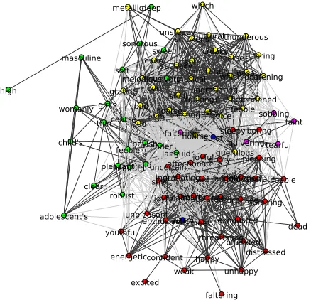
5.3 Clustering with the Spin Glass Community Detection on Graphs
For comparison with Affinity Propagation meth-ods, we use community detection algorithms on semantic similarity graphs. First, a graph is con-structed, in which the words (the headword and its collocates) are vertexes. Then, for each pair of vertexes, we calculate their cosine similarity in the current word embedding model. If it exceeds a pre-defined threshold, an edge between these two vertexes is added to the graph with the cosine sim-ilarity value as the edge weight.8
TheSpin glasscommunity detection algorithm
7In our preliminary experiments, we tried to useK-Means for the second step, but it performed worse than spectral clus-tering.
8The threshold is automatically adapted for each head-word separately, based on the average cosine similarity be-tween pairs of its collocates; thus, in more semantically ‘dense’ sets of collocates, the threshold is higher.
excited boyish surprised boring girl's joyful creaky soft affectionate quiet shrill youthful faltering sweet deafening masculine happy unnaturally faltering beautiful adolescent's husky frightened robust smoker's thunderous unhappy which angry hoarse exhausted womanly hoarse joyful sad tearful croaking coarse velvety offended hoarse hearty sonorous deadened pleasant soft angry sleepy distressed old admiring ingratiating quivering faltering weak sobbing feeble which child's feeble enthusiastic musical metallicdeep faint loud ingratiating agitatedtired dead grating uncertain warm feeble querulous loud desperate pleading unsteady languid squeaky clear thin tender nasal guttural high meek high shy threatening piercing confident energetic calm loud unpleasant even muffled melodious voice
Figure 2: Clustering of the collocates for ‘голос’
(voice) by theSpin glassalgorithm.
was employed to find clusters in the graph. Spin glasscannot process unconnected graphs; thus, if this is the case (about 10-15% of the headwords in the gold standard), we fall back to theInfomap community detection algorithm; with connected graphs, it performs worse thanSpin glass. We use the implementations of the community detection algorithms in the Igraph library (Csardi and Ne-pusz, 2006), and the whole gold standard as a de-velopment set to fine-tune the hyperparameters of the algorithms. Figure 2 shows the results of graph clustering for ‘голос’ (voice) headword, with
dif-ferent clusters shown in colors and edge widths representing cosine similarities. The visualization shows that the similarities between words belong-ing to one cluster are on average higher than those on the inter-cluster edges.
6 Results
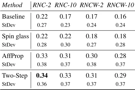
[image:6.612.317.536.42.253.2]Table 1: Clustering evaluation, average ARI and standard deviation
Method RNC-2 RNC-10 RNCW-2 RNCW-10 Baseline 0.22 0.17 0.17 0.16
StDev 0.27 0.23 0.24 0.24
Spin glass 0.22 0.22 0.18 0.18
StDev 0.28 0.30 0.27 0.28
AffProp 0.33 0.31 0.30 0.28
StDev 0.38 0.37 0.38 0.37
Two-Step 0.34 0.33 0.31 0.29
StDev 0.36 0.37 0.37 0.37
perfect correspondence between the gold standard and the clustering; -1 means negative correlation; 0 means the clustering and the gold standard are not related to each other.
We compute ARI individually for each head-word and then average over all 63 entries. The Table 1 presents the evaluations results. RNC-2 and RNC-10 stand for the word embedding mod-els trained on the RNC with symmetric window 2 and 10 respectively; RNCW stands for the respec-tive models trained on the RNC and the Russian Wikipedia together.Spin glassis the method using communities detection on graphs (Section 5.3), AffProp is the single-step Affinity Propagation clustering (Section 5.2), andTwo-Stepis our pro-posed approach of cascade clustering. We also re-port the standard deviation of the individual head-words ARI for each approach (StDev).
As can be seen from the table, the baseline, which is a simple clustering of word embeddings, is difficult to beat. The graph-based community detection algorithm performs on par with the base-line on the models with window size 2 and only slightly outperforms it on the models with win-dow 10. However, using the fine-tuned Affin-ity Propagation makes a huge difference, push-ing ARI higher by at least 10 decimal points for all models. Feeding the number of clusters de-tected by theAffinity Propagationinto the spectral clustering algorithm (ourTwo-Stepapproach) con-sistently increases the performance by one point more. Note that theTwo-Stepmethod is also con-siderably faster than the graph-basedSpin glass al-gorithm.
It is worth noticing that the larger window
mod-els consistently perform worse in this task. It seems that the reason is exactly that they pay more attention to broad associative relatedness between words and less to direct functional or paradigmatic similarity. But this is precisely what is important in the task of clustering collocates: we are try-ing to find groups of adjectives which can roughly substitute each other in modifying the headword noun. For example, ‘beautiful’ and ‘charming’ are equally suitable to characterize a pretty face, but ‘beloved face’ does not belong to the same con-struction; however, in the models with larger win-dow size ‘beautiful’ and ‘beloved’ are very close and will fall into the same cluster.
At the same time, the variance among head-words may be higher than the variance be-tween models. For example, in our experiments, for the headword ‘ступня’ (foot/sole), all four
methods—two-step and spin glass on the RNC2 and the RNC10—yield ARI 0.816 and produce identical results. At the same time, for the head-word ‘живот’ (stomach/belly) all four methods
produced negative ARI, which probably means that clustering for this headword is especially dif-ficult to predict.
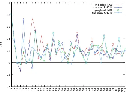
In Figure 3 we present individual headwords ARI for the 4 best performing methods. The head-words in the plot are sorted by the number of col-locates. The headwords with less than 10 collo-cates are excluded from the plot: these smaller entries are more diverse and in many cases yield ARI=0 or ARI=19. It can be seen from the figure
that for many headwords ARI from different meth-ods are almost identical and there are clear ‘easy’ and ‘difficult’ headwords. The more collocates the headword has the closer are the results produced by different approaches. Similar variability among headwords was observed before in various MWE-related tasks (Pivovarova et al., 2018); we assume that this can be at least partially explained by dif-ferent abilities of words to form stable MWEs. Nevertheless, it can be seen from Figure 3 that in most cases ARI is higher than zero, pointing at sig-nificant correlation between the gold standard and the automatic clustering.
Another interesting finding is that the models trained on the RNC and Wikipedia together show worse results than the models trained on the RNC only, as can be seen from Table 1. Thus, despite
9However, all 63 headwords were used to compute the average values in Table 1.
-0.4 -0.2 0 0.2 0.4 0.6 0.8 1
10 13 14 14 15 15 17 18 19 20 22 22 25 25 29 29 30 33 33 33 34 36 37 38 39 43 46 49 50 53 58 59 63 66 73 81 100 123 140
ARI
number of collocates
[image:8.612.85.521.41.359.2]two-step RNC2 two-step RNC10 spinglass RNC2 spinglass RNC10
Figure 3: Individual headwords ARI for 4 best-performing methods; the headwords are sorted by the number of collocates.
the fact that the training corpus was more than two times larger, it did not result in better embeddings. This seems to support the opinion in (Kutuzov and Andreev, 2015) that when training distributional models, versatile and balanced nature of the cor-pus might be at least as important as its size.
Using our Two-Step algorithm and the RNC-2 model, we produced clusterings for all ‘adjec-tive+noun’ bigrams in the RNC with PPMI more than 1, the corpus frequency of the bigram more than 10 and the frequency of the nominal head-word more than 1 000. This corresponds to 6 036 headwords and 143 314 bigrams (headwords with only 1 collocate were excluded). We publish this dataset online together with our gold standard on the home page of the CoCoCo project10. For
bet-ter cross-linguistic comparability, all PoS tags in these datasets were converted to the Universal PoS Tags standard (Petrov et al., 2012).
This clustering was evaluated against our gold
10Collocations, Colligations, Corpora, http://cosyco.ru/cococo/
standard (A Russian-English Collocational Dictio-nary of the Human Body) as well. We had to work only with the intersection of the gold standard data and the resulting clustering, thus only a part of the gold standard was actually used for the eval-uation (59 headwords out of 63, and 966 collo-cations out of 1758). It produced ARI=0.38 cal-culated on all headwords and ARI=0.31after we excluded 6 headwords that have only one collo-cate in this dataset—their evaluation always pro-duces ARI=1, independent of what the clustering algorithm outputs. These results confirm that the proposed algorithm performs well not only on the limited artificial data from the gold standard, but on the real world data.
Note that this is partial evaluation and many bigrams are left unattended. For example, for the headword ‘лицо’ (face), the collocates
‘увядший’ (withered) and ‘морщинистый’
tion to compute ARI. However, in the complete clustering results these collocates are also grouped together with some other words not present in the gold standard: ‘сморщенный’ (withered) and
‘иссохший’ (exsiccated), which is probably
cor-rect, and ‘отсутствующий’ (absent), which is
obviously wrong. As the dictionary lacks these collocates, they cannot affect the evaluation re-sults, whether they are correct or incorrect. After analyzing the data, we can suggest that the clus-tering quality of the complete RNC data is more or less the same as it was for the dictionary data, but more precise evaluation would require a man-ual linguistic analysis.
7 Conclusion
The main contributions of this paper are the fol-lowing:
1. We investigated MWE analysis techniques beyond collocation extraction and proposed a new approach to automatic construction ex-traction;
2. Several word embedding models and vari-ous clustering techniques were compared to obtain MWE clustering similar to manual grouping with the highest ARI value being 0.34;
3. We combined two clustering algorithms, namely the Affinity Propagation and the Spectral Clustering, to obtain results higher than can be achieved by each of this methods separately;
4. The best algorithm was then applied to clus-ter all frequent ‘adjective+noun’ bigrams in the Russian National Corpus. The obtained clusterings are publicly available and could be used as a starting point for constructional studies and building construction dictionar-ies, or utilized in various NLP tasks.
The main inference from our experiments is that the task of clustering Russian bigrams into constructions is a difficult one. Partially it can be explained by the limited coverage of the gold standard, but the main reason is that bigrams are grouped in non-trivial ways, that combine seman-tic and syntacseman-tic dimensions. Moreover, the num-ber of clusters in the gold standard varies among headwords, and thus should be detected at the test
time, adding to the complexity of the task. How-ever, it seems that distributional semantic mod-els can still be used to at least roughly reproduce manual grouping of collocates for particular head-words.
We believe that automatic construction extrac-tion is a fruitful line of research that may be help-ful both in practical applications and in corpus lin-guistics, for better understanding of constructions as lexical-semantic units.
In future we plan to explore other constructions besides ‘adjective + noun’; first of all we plan to start with the ‘verb+noun’ constructions, since they are also present in the dictionary used as the gold standard. We would also try to find or com-pile other gold standards, since the dictionary we use is limited in its coverage; for example, the authors allowed only literal physical meanings of the words in the dictionary, intentionally ignoring metaphors.
In all our experiments, we used embeddings for individual words. However, it seems natu-ral to learn embeddings for bigrams since they may have quite different semantics than individ-ual words (Vecchi et al., 2016). It is crucial to de-termine bigrams that need a separate embedding and/or try to utilize already learned embeddings for individual words11.
Another interesting topic would be cluster la-beling, which is finding the most typical rep-resentative of a construction, or a construction name. The Affinity Propagation outputs exem-plars for each cluster, but these exemexem-plars are not always suitable as cluster labels. For example, for the headword ‘ступня’ (foot) the algorithm
correctly identifies the following group of adjec-tive modifiers: [‘широкий’ (wide), ‘узкий’ (
nar-row), ‘большой’ (large), ‘маленький’ (small),
‘изящный’ (elegant)] with ‘узкий’ (narrow)
be-ing the exemplar for this class. However, in the dictionary this group is labeled ‘Size and shape; aestetics’, which is more suitable from the human point of view. Some kind of an automatic hyper-nym finding technique is necessary for this task.
Finally, we plan to use hierarchical cluster-ing algorithms to obtain a more natural structure of high-level constructions split into smaller sub-groups.
References
Timothy Baldwin and Aline Villavicencio. 2002. Ex-tracting the unextractable: A case study on verb-particles. InProceedings of the 6th conference on Natural language learning, volume 20, pages 1–7. Association for Computational Linguistics.
Marco Baroni, Georgiana Dinu, and Germán Kruszewski. 2014. Don’t count, predict! a systematic comparison of context-counting vs. context-predicting semantic vectors. InProceedings of the 52nd Annual Meeting of the Association for Computational Linguistics (Volume 1: Long Papers), pages 238–247.
Lars Borin, Linnéa Bäckström, Markus Forsberg, Ben-jamin Lyngfelt, Julia Prentice, and Emma Sköld-berg. 2013. Automatic identification of construc-tion candidates for a Swedish Constructicon. In
Proceedings of the workshop on lexical semantic re-sources for NLP at NODALIDA 2013, number 088, pages 2–11. Linköping University Electronic Press. Wei-Te Chen, Claire Bonial, and Martha Palmer. 2015.
English light verb construction identification using lexical knowledge. InAAAI, pages 2368–2374. Kenneth Church, William Gale, Patrick Hanks, and
Donald Kindle. 1991. Using statistics in lexical analysis. Lexical acquisition: exploiting on-line re-sources to build a lexicon, page 115.
Gabor Csardi and Tamas Nepusz. 2006. The Igraph software package for complex network research. In-terJournal, Complex Systems, 1695(5):1–9.
Charles J. Fillmore, Paul Kay, and Mary Catherine O’Connor. 1988. Regularity and idiomaticity in grammatical constructions: The case of let alone.
Language, pages 501–538.
John R. Firth. 1957. A synopsis of linguistic theory, 1930-1955. studies in linguistic analysis. Oxford: Philological Society. [Reprinted in Selected Papers of J.R. Firth 1952-1959, ed. Frank R. Palmer, 1968. London: Longman].
Santo Fortunato. 2010. Community detection in graphs.Physics reports, 486(3):75–174.
Brendan J. Frey and Delbert Dueck. 2007. Clustering by passing messages between data points. Science, 315(5814):972–976.
Stefan Th. Gries and Anatol Stefanowitsch. 2004. Ex-tending collostructional analysis: A corpus-based perspective on alternations’. International journal of corpus linguistics, 9(1):97–129.
Lawrence Hubert and Phipps Arabie. 1985. Compar-ing partitions. Journal of classification, 2(1):193– 218.
Lidija Iordanskaja, Slava Paperno, Lesli LaRocco, Jean MacKenzie, and Richard L. Leed. 1999.A Russian-English Collocational Dictionary of the Human Body. Slavica Publisher.
Oskar Kohonen, Sami Virpioja, and Krista Lagus. 2009. Constructionist approaches to grammar infer-ence. In NIPS Workshop on Grammar Induction, Representation of Language and Language Learn-ing, Whistler, Canada.
Mikhail Kopotev, Lidia Pivovarova, and Daria Ko-rmacheva. 2016. Constructional generalization over Russian collocations. Mémoires de la Société néophilologique de Helsinki, Collocations Cross-Linguistically:121–140.
Andrey Kutuzov and Igor Andreev. 2015. Texts in, meaning out: neural language models in semantic similarity task for Russian. InComputational Lin-guistics and Intellectual Technologies: papers from the Annual conference "Dialogue", volume 14(21). RGGU.
Ira Leviant and Roi Reichart. 2015. Separated by an un-common language: Towards judgment language informed vector space modeling. arxiv preprint.
arXiv preprint arXiv:1508.00106.
Omer Levy and Yoav Goldberg. 2014. Dependency-based word embeddings. InProceedings of the 52nd Annual Meeting of the Association for Computa-tional Linguistics (Volume 2: Short Papers), pages 302–308.
Igor Mel’cuk. 1995. Phrasemes in language and phraseology in linguistics. Idioms: Structural and psychological perspectives, pages 167–232. Tomas Mikolov, Ilya Sutskever, Kai Chen, Greg S.
Cor-rado, and Jeff Dean. 2013. Distributed representa-tions of words and phrases and their compositional-ity. InAdvances in Neural Information Processing Systems 26, pages 3111–3119. Curran Associates, Inc.
Jeff Mitchell and Mirella Lapata. 2008. Vector-based models of semantic composition. In Proceedings of ACL-08: HLT, pages 236–244. Association for Computational Linguistics.
Andrew Y. Ng, Michael I. Jordan, and Yair Weiss. 2001. On spectral clustering: Analysis and an al-gorithm. InAdvances in Neural Information Pro-cessing Systems, pages 849–856. MIT Press. F. Pedregosa, G. Varoquaux, A. Gramfort, V. Michel,
B. Thirion, O. Grisel, M. Blondel, P. Prettenhofer, R. Weiss, V. Dubourg, J. Vanderplas, A. Passos, D. Cournapeau, M. Brucher, M. Perrot, and E. Duch-esnay. 2011. Scikit-learn: Machine learning in Python. Journal of Machine Learning Research, 12:2825–2830.
Jing Peng, Anna Feldman, and Hamza Jazmati. 2015. Classifying idiomatic and literal expressions using vector space representations. In Proceedings of the International Conference Recent Advances in Natural Language Processing, pages 507–511. IN-COMA Ltd. Shoumen, BULGARIA.
Slav Petrov, Dipanjan Das, and Ryan McDonald. 2012. A universal part-of-speech tagset. In Proceedings of the Eighth International Conference on Language Resources and Evaluation (LREC-2012). ELRA. Lidia Pivovarova, Daria Kormacheva, and Mikhail
Kopotev. 2018. Evaluation of collocation extraction methods for the Russian language. InQuantitative Approaches to the Russian Language. Routledge. Radim ˇReh˚uˇrek and Petr Sojka. 2010. Software
Framework for Topic Modelling with Large Cor-pora. InProceedings of the LREC 2010 Workshop on New Challenges for NLP Frameworks, pages 45– 50, Valletta, Malta. ELRA.
Jörg Reichardt and Stefan Bornholdt. 2006. Statis-tical mechanics of community detection. Physical Review E, 74(1):016110.
Martin Rosvall, Daniel Axelsson, and Carl T. Bergstrom. 2009. The map equation.The European Physical Journal Special Topics, 178(1):13–23. Ilya Segalovich. 2003. A fast morphological algorithm
with unknown word guessing induced by a dictio-nary for a Web search engine. In MLMTA, pages 273–280.
Yuancheng Tu and Dan Roth. 2011. Learning En-glish light verb constructions: contextual or statis-tical. InProceedings of the Workshop on Multiword Expressions: from Parsing and Generation to the Real World, pages 31–39. Association for Compu-tational Linguistics.
Peter D. Turney and Patrick Pantel. 2010. From frequency to meaning: Vector space models of se-mantics. Journal of artificial intelligence research, 37(1):141–188.
Laurens Van der Maaten and Geoffrey Hinton. 2008. Visualizing data using t-SNE. Journal of Machine Learning Research, 9(2579-2605):85.
Eva M. Vecchi, Marco Marelli, Roberto Zamparelli, and Marco Baroni. 2016. Spicy adjectives and nom-inal donkeys: Capturing semantic deviance using compositionality in distributional spaces. Cognitive science.
Veronika Vincze, Istvan T. Nagy, and Richárd Farkas. 2013. Identifying English and Hungarian light verb constructions: A contrastive approach. In Proceed-ings of the 51st Annual Meeting of the Association for Computational Linguistics (Volume 2: Short Pa-pers), pages 255–261.