Developing a Surrogate-Based Time-Averaged
Momentum Source Model from 3D CFD
Simulations of Small Scale Propellers
Joseph Carroll,
Member, IAENG
and David Marcum
Abstract—Many Miniature Aerial Vehicles (MAV) are driven by small scale, fixed blade propellers which can have significant impact on MAV aerodynamics. In the design and analysis process for MAVs, numerous computational fluid dynamic (CFD) simulations of the coupled aircraft and propeller are often conducted which require a time averaged, steady-state approximation of the propeller for computational efficiency. Most steady state propeller models apply an actuator disk of momentum sources to model the thrust and swirl imparted to the flowfield by a propeller. The majority of these momentum source models are based on blade element theory. Blade element theory discretizes the blade into airfoil sections and assumes them to behave as two-dimensional (2D) airfoils. Blade element theory neglects 3D flow effects that can greatly affect propeller performance limiting its accuracy and range of application.
In this paper, surrogate models for the time averaged thrust and swirl produced by each blade element are trained from a database of time-accurate, high-fidelity 3D CFD propeller simulations. Since the surrogate models are trained from these high-fidelity CFD simulations, various 3D effects on propellers are inherently accounted for such as tip loss, hub loss, post stall effect, and element interaction. These surrogate models are functions of local flow properties at the blade elements and are embedded into 3D CFD simulations as locally adaptive momentum source terms. Results of the thrust profiles for the steady-state surrogate propeller model are compared to the time-dependent, high-fidelity 3D CFD propeller simulations coupled to an aircraft. This surrogate propeller model which is dependent on local flowfield properties simulates the time-averaged flowfield produced by the propeller and captures the 3D effects and accuracy of time-dependent 3D CFD propeller blade simulations but at a much lower cost.
Index Terms—Surrogate, Propeller, blade element, computa-tional fluid dynamics.
I. INTRODUCTION
M
INIATURE Aerial Vehicles (MAV) are becoming increasingly popular in the military and domestic sectors. Many of these MAVs use small scale, fixed blade propellers for propulsion. Computational Fluid Dynamic (CFD) analysis is heavily used in the design and analysis process for these aircraft. Hundreds of CFD simulations are often conducted to determine the aerodynamic coefficients of the aircraft. Depending on the mounting configuration and sizing of the propeller, the propeller-aircraft interaction can be strongly coupled thus the propeller and aircraft must be simulated together. In many instances, the aerodynamic performance of the aircraft is significantly affected by theManuscript received on Feb 26, 2013; accepted on March 19, 2013 Joseph Carroll is a Ph.D. student with the Department of Mechanical En-gineering at Mississippi State University funded through CAVS, Starkville, MS, 39762 USA e-mail: [email protected]
David Marcum is a Professor with the Department of Mechanical Engi-neering at Mississippi State University, e-mail: [email protected]
wake of the propeller and thus an accurate model of the flow produced by the propeller is needed.
The CFD simulation of a propeller can be performed in various ways ranging in levels of complexity. The most detailed and accurate method is to use high-fidelity 3D CFD of viscous, compressible flow to conduct a time-dependent simulation in which the propeller is rotated relative to the aircraft. For compactness, this method will be referred to in this paper as the High-Fidelity Blade Model (HFBM). HFBM gives a highly detailed, time-accurate flowfield so-lution which comes at a great computational expense. The high cost often makes this detailed and accurate method of modeling infeasible when numerous simulations are needed as is the case in determining the aerodynamic coefficients for an aircraft.
A steady-state, computationally efficient method of simu-lating a propeller is to view the propeller in a time-averaged sense as a source of momentum imparted to the flow. The time averaged thrust and swirl produced by a propeller is implemented into 3D CFD by embedding momentum source terms in the propeller region of the mesh. These momentum source terms are based on simplified propeller theories such as blade element theory. Blade element theory momentum source term models are well documented in literature [1]– [3]. However, these simplified theories fail to capture many of the complex 3D flow characteristics which can affect propeller performance, limiting their accuracy and range of applicability. A need exists for a low cost, steady-state propeller model which captures the accuracy of HFBM but is applied at the momentum source level of detail.
II. 3D EFFECTS ON APROPELLER
Propeller aerodynamics are quite complicated and have highly 3D flowfields. The finiteness of the blade yields complex flows around the tip. Flow circulates from the high pressure to the low pressure side causing tip vortices to be introduced into the propeller wake. These tip vortices have a detrimental effect on the thrust of a blade in the tip region; this is known as tip loss. Different blade tip geometries and propeller operating conditions result in different tip losses. In addition to tip loss, flow around the hub can also introduce vortices or flow in the spanwise direction which affects propeller performance by altering the local flow characteristics at the blade similar to a tip vortex.
The rotation of the propeller causes significant centrifugal and coriolis forces on the blade and thus on the fluid particles close to the blade surface through viscous effects. Centrifugal force causes the boundary layer to have large outward spanwise components. The coriolis force is stabilizing to the boundary layer much like a favorable pressure gradient [4]. Due to the effects of these rotational forces in the boundary layer, separation on a 3D rotating propeller blade is postponed to higherαcompared to that of a nonrotational flowfield. This effect known as stall-delay is strongest near the root and decreases towards the tip proportional to increas-ing radial position. This delayed separation caused by 3D rotational effects has a favorable effect on propeller thrust.
III. BLADEELEMENTTHEORY
Blade element theory is the most common method for propeller modeling. It divides the blade into many sections in the spanwise direction which are assumed to be independent of one another. The blade elements are assumed to operate as a 2D wing in a 2D flowfield. Lift and drag characteristics of the airfoil at each blade element are used to calculate the thrust and swirl imparted to the flowfield as functions of the localα,Re, andM. The flight velocity and rotational speed of the propeller are known, however the induced velocity components are unknown. Therefore, blade element theory must be combined with another theoretical model to calculate these induced velocities. Many models exists for calculating the induced velocities such as those based on momentum theory, lifting-line theory, and a number of vortex models which describe the propeller wake in varying levels of detail. Fundamentally, the blade element theory assumes the flow over each element to be independent and 2D in nature. However, as previously discussed, propeller aerodynamics can be highly 3D and thus not accurately predicted by 2D airfoil data. Correction models must be coupled with the blade element theory in order to compensate for errors from the simplifying 2D flow assumption and the theoretical induction models. Numerous tip loss, hub loss, and stall-delay models exist in an attempt to correct blade element models for 3D effects. However, these correction models are often empirically based and have a very limited range of applicability.
IV. COMPARINGBLADEELEMENTTHEORY TOHFBM
To show the error associated with blade element models, the popular Glauret’s Blade Element Momentum (BEM) model and HFBM are applied to a small scale, two blade
Fig. 1: Small scale propeller used for simulation
propeller with a 25.4 cm diameter shown in Figure 1 . The thrust profile obtained from the blade element code is compared to a HFBM of the propeller in uniform flow with no other bodies in the domain. Prandtl’s tip and hub loss correction models are applied to Glauret’s BEM model which are widely. Details for the Glauret’s model along with the correction factors can be found in the cited reference [5].
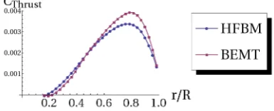
[image:2.595.330.523.479.557.2]For a direct comparison, the 2D airfoil simulations used in the blade element code and the HFBM simulation are both conducted using an in-house code at Mississippi State University (MSU) called CHEM [6]. CHEM is a second-order accurate, cell-centered finite volume CFD code and has been validated and applied to a wide range of problems. All CFD simulations are compressible, viscous and assumed to be turbulent using Menters shear stress transport (SST) turbulence model. While theReis low (<150,000), the SST turbulence model is used to achieve settled solutions since unsteady vortex shedding occurs in regions of separation on the blade. A y+ < 5 is maintained in the first cell off the viscous surfaces for all simulations, and the point spacing for the mesh on the 2D airfoil and any blade cross section on the 3D mesh is similar. The 2D airfoil data base spans a sufficient range ofαandRewhich is experienced by all the blade elements. Mach number is not varied since the tip mach number is sufficiently small to neglect compressibility effects (<0.15). A moderate advance ratio of 0.29 is simulated to prevent large regions of separation on the blade. Figure 2 shows the thrust profile comparison. A combination of post
Fig. 2: BEM model vs. HFBM
stall and hub effects are seen near the root as BEM under predicts the thrust in this inboard region. In addition, the tip effect on this propeller affects a significant portion (r/R > 0.6) of blade. Even though Prandtl’s tip loss model is used in the BEM code, there is significant error in the tip region. Many small scale propellers have low aspect ratio blades which exaggerate the tip loss. The average error over all the blade elements is quantified using a Root Mean Square Error (RMSE) which is normalized by the total thrust produced by the propeller in HFBM as shown in equation 1 .
RM SE= 1
T hrusttotal 1
N N
X
i=1
q
(fi−fˆi)2 (1)
in accurately predicting small propeller thrust profiles from blade element theory even with correction models. Other work supports this comparison by showing the discrepan-cies between blade element predictions to experimental and HFBM simulations for small scale UAV propellers [7], [8].
V. SURROGATEMODELINGPROCEDURE
A. Motivation
In a basic sense, surrogate simply means substitute, or one that takes the place of another. In the area of modeling, surrogate refers to an inexpensive approximation of a de-tailed, expensive computation. This efficient approximating function is developed by interpolating data from a few select cases of the expensive, high-fidelity computations. The up front cost to perform the limited number of ex-pensive training cases and develop the surrogate may be time consuming. Nonetheless, this initial expense is cheaper than repeating the expensive computation numerous times. Surrogate modeling is applied to many disciplines, and is widely used in aerospace engineering. Performing numerous coupled propeller-aircraft HFBM simulations lends itself to a surrogate modeling of the propeller as an efficient yet accurate approximation is needed.
The surrogate-based model accounts for 3D effects such as tip loss, hub loss, and post stall effects since the training method is a 3D solution of the Navier-Stokes equations over the computational domain through the use of CFD. Contrary to blade element theory, each blade element has its own surrogate models for thrust and swirl. Therefore, no corrections models are needed to approximate the 3D effects as they are “built-in” to the training method. Applying the surrogates as steady-state models significantly reduces computation time since the problem is no longer restricted to operate on the small time step which is needed to resolve the fast propeller rotation. The mesh size is drastically reduced as there is no need to create a mesh over the propeller blade since it is approximated by momentum sources. In addition, making the surrogates functions of local flowfield variables allows the model to adjust to different flight attitudes and aircraft couplings.
B. HFBM Training Simulations
The CHEM code is used to perform the all the HFBM training simulations. The unstructured grid generator AFLR3 [9], [10] is used to make all the meshes. The same propeller used in the BEM versus HFBM comparison. Training simulations model the propeller in uniform flow (0 α relative to the propeller) with no other bodies in the domain. If the mounting configuration and aircraft is known and will not change throughout the application of the model, the training cases could be propeller-aircraft coupled simulations. However, an important quality of train-ing simulations are their generality, or ability to model a wide of range of applications. Therefore, it is undesirable to restrict the training simulations to one aircraft and mounting configuration. Simulating a wide variety of isolated propeller cases covers a wide range of influential flow characteristics which will be used as surrogate model inputs. This range of inputs spanned by isolated propeller simulations includes the majority of those induced by the presence of an aircraft
thus allowing these general training cases cover numerous propeller-aircraft coupling situations.
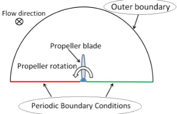
[image:3.595.336.515.215.330.2]Since the flow is uniform, the propeller problem is ax-isymmetric about the rotational axis. This means that the flow seen by each blade is similar and steady-state in the fixed blade reference frame. Since each blade experiences rotational periodicity, only one blade needs to be modeled and the problem size can be reduced proportional to the number of blades. Therefore, periodic boundary conditions are used on the axisymmetric planes. Figure 3 shows a front view onto the rotational axis for HFBM simulations setup. All training simulations are compressible, viscous and
Fig. 3: Periodic domain for HFBM training simulations
assumed to be turbulent using Menters shear stress transport (SST) turbulence model. The boundary layer grid is refined so that y+ < 5 in the first cells off the viscous surfaces for all training cases. The entire grid is rotated for time-dependent simulations in which 1◦ of rotation corresponds to 1 time-step. Each time step is refined with a number of Gauss-Seidel iterations to ensure temporal accuracy over each time-step. Simulations are run for at least 5 revolutions to achieve settled solutions without start-up effects.
C. Extracting Inputs and Outputs from Training Cases
The propeller blade is discretized into 30 blade element sections which individual surrogate models describe. To extract the outputs of axial and tangential forces (thrust and swirl) on each blade element, the surface of the blade is divided into the element sections and the CHEM code outputs output the integrated forces (viscous + inviscid) over each blade element.
A propeller blade is simply a rotating wing and it is well known that α, Re, and M are main the parameters that affect the lift and drag of a wing and similarly thrust and swirl of a propeller. As with most small scale propellers, the mach number is small, < 0.25 for the case in this paper. Compressibility effects are assumed to be negligible thus only localαandRe are considered as inputs to the model. It is imperative that the inputs be extracted locally at the blade element sections to allow the surrogate models to be adaptive to local changes in flowfield parameters which can be induced by different aircraft coupling configurations.
averages of velocity vectors are taken just upstream of the propeller. Figure 4 shows an annulus for a corresponding blade element over which the velocity vectors are averaged. The inputs are averaged at a constant axial position a
Fig. 4: Annulus region over which to take a circumferential average of the velocity vectors
small distance upstream (7.8% of the propeller radius) from the propeller plane. This upstream position for the input extraction prevents the averaging annulus from intersecting the propeller blade allowing for a simple circumferential averaging. However, the upstream position is still close enough to the propeller so the inputs are local to each blade element and can be influenced by obstructions downstream of the propeller.
After a circumferential average of the velocity vectors, each blade element has one time-averaged local velocity vector. From this velocity vector, the local α and Re can be determined for each blade element which are used as the inputs to the surrogate model. Extracting the inputs and outputs for all the training cases gives an input-output database from which a surrogate model can be developed.
D. Optimization of the Surrogate Model
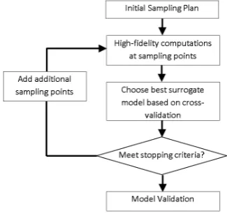
Developing a cheap surrogate model to accurately and efficiently predict the response of high-fidelity simulations over a design space depends on several factors such as the form of the surrogate model and locations of the training cases in the sampling space. An optimization process is conducted to ensure an efficient coverage of the sampling space1and optimal choice of the surrogate model by reducing the global error in an iterative manner [12]. The process is outlined in Figure 5. The sampling space is 2D with advance ratio (J) and rotational speed (rotations per minute -rpm) as the two variables for the simulations. Changing these global simulation parameters ofJ andrpm varies the localαand andRerespectively at each blade element. The bounds of the simulation parameters are chosen for a typical flight envelope of the propeller.Jranges from 0 to 0.6, andrpmranges from 2000 to 6500. An Optimal Latin Hypercube (OLH) algorithm is used to create the initial sampling plan of 10 points since it has a desirable space filling property. The best surrogate model for this initial sampling plan is chosen based on leave-one-out cross-validation (LOOCV). In LOOCV, the sampling plan is divided into k subsets in which each subset leaves one sampling point out. Surrogate models are trained for each subset and then validated against the point that was left
1Thanks to Frederic Alauzet for suggesting sampling space optimization
out of that particular subset. Error estimates for the propeller thrust are determined at each point by equation 1 . Averaging the local error at each point in the sampling plan results in a a global error estimation for the surrogate model. The points that make up the convex hull of the sampling plan are not included in the LOOCV error estimation process as extrapolation would occur at these points resulting in an over estimation of the error at the boundary. The mean error over all the points included in the LOOCV are assigned to the error at the convex hull points.
Polynomial regression models are used for the surrogates as the input-output relationship is relatively smooth and without spikes in the data. To determine the best form of the polynomial equation, Mathematica is used to create each possible polynomial form consisting of the different combinations of terms up to third order. The polynomial form is restricted to third order to prevent unrealistic oscillations and erratic behavior if extrapolation occurs. The form with the smallest global error according to LOOCV is chosen as the best surrogate model.
A surface map of the surrogate’s error over the sampling space is created using linear a radial basis function (RBF). Additional space filling candidate points are added which consider the existing sampling plan to maintain the space filling property. The RBF is used to predict the error at each candidate point andnpoints with the highest error are added to the sampling plan. n is selected to be 3 for this problem, but can be adjusted based on simulation to surrogate evaluation turn around time. This optimization process of the surrogate and adaptive sequential sampling plan is repeated until the global error of the surrogate is sufficiently small, <1%for this case. Only one iteration was required to meet the stopping criteria of RMSE<1%.
E. Implementing the model as momentum sources
The general form of the conservation equation of fluids for a variableφis shown in Equation 2 .
∂(ρφ)
∂t + ∂ ∂xi
(ρUiφ−Γiφ ∂φ ∂xi
)−Sφ= 0 (2)
Surrogate models for the thrust and swirl imparted to the flow are applied as momentum source terms (Sφ) into 3D CFD simulations. The CFD software ANSYS FLUENT is chosen to implement the model since it has convenient and
[image:4.595.337.500.605.758.2]easy to use User Defined Functions (UDFs) for adding source terms to the flow. Source terms are applied explicitly on a per-volume basis in the propeller region of the mesh which is a cylinder approximately the same thickness and exactly the same diameter of the propeller. The mesh in the propeller region is refined to distribute the source terms over several cells in the axial direction. Distributing the source terms uniformly in the axial direction provides a smooth, stable increase in momentum across the propeller region.
[image:5.595.336.514.63.208.2] [image:5.595.81.260.253.356.2]Inputs for the source terms are calculated from flow variables in cells just upstream of the propeller region. Figure 6 shows a cross section of the grid for implementing the surrogate-based source terms. This figure highlights the propeller region in which the source terms are applied and the location of the cells whose flow variables are used as inputs for the source terms. The location from which to
Fig. 6: Grid for surrogate model
extract the local inputs is adjusted a small amount from the training simulations. This slight adjustment of the input location is needed as the source terms are applied over a constant thickness propeller region which is not an exact representation of the propeller. Coupling the source terms to local flowfield variables allows the sources to adapt as the solution progresses. Adaption through the local inputs enables the surrogate propeller model to account for a wide range of aircraft couplings.
VI. RESULTS ANDDISCUSSION
Simulations of the surrogate model are compared to a HFBM for the small scale propeller coupled to a MAV. The propeller operates at a moderate advance ratio of 0.275 and the MAV is at 0 angle of attack. The CHEM code is used to perform the HFBM simulation and FLUENT is used to perform the surrogate model simulation. The two codes are comparable and both use 2nd order differencing. A tractor type mounting position is chosen in which the propeller is very close to the leading edge of the MAV. The close coupling ensures a strong two-way interaction between the propeller and MAV. Figure 7 shows a picture of the test case. The radial distribution of thrust and swirl along the blade is compared between simulations when the propeller is in two positions as shown in Figure 8. Figure 9 shows
Fig. 7: MAV-propeller test case
(a) Vertical position
(b) Horizontal position
Fig. 8: Propeller positions for comparing results
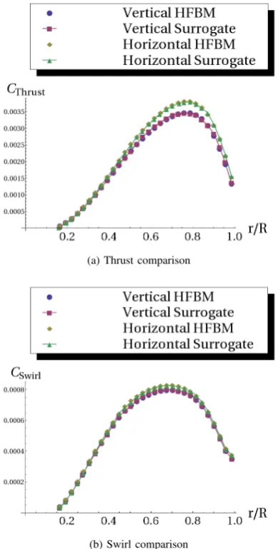
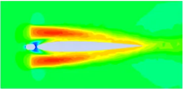
the comparison of thrust and swirl between the surrogate model and HFBM for both the horizontal and vertical pro-peller positions. In addition, Figure 10 shows a picture of the velocity contours over a cross section from surrogate model simulation to see the flowfield induced by the source terms. The surrogate model predicts the thrust and swirl in both propeller positions with near perfect agreement to HFBM. Notice the accuracy of the surrogate model compared to HFBM in the tip and hub regions. This demonstrates the capability of the model to accurately account for the
(a) Thrust comparison
[image:5.595.329.524.370.755.2](b) Swirl comparison
[image:5.595.87.252.707.761.2]Fig. 10: Velocity contours for cross section of the MAV simulation with the surrogate model
complicated 3D effects. The average error in thrust between both positions is 0.67% as calculated by equation 1 and is a significant improvement from the 12% error associated with the blade element theory for an isolated propeller at this flight condition. This low error is not a surprise as the stopping criteria for the ASS plan is error<1%.
In the horizontal position, the thrust is higher because the propeller is sweeping through the flowfield directly in front of the MAV. Flow in the axial direction approaching the MAV slows down causing the propeller to operate at a higher angle of attack which results in a greater thrust than the vertical position. The surrogate model accurately predicts this higher thrust in the horizontal position. This highlights the capability of the local flowfield inputs to adapt the propeller performance to mounting configurations with strong aircraft-propeller coupling.
Recall that the training cases only consist of HFBM simulations with no other bodies in the flow. The wide range of α andRe spanned by the training cases for each blade element cover even the inputs induced by the MAV when the propeller is in the horizontal position. The range of α covered by the training simulations for each blade element is compared to the spanwiseαdistribtion for both positions as shown in Figure 11. Theseα distribtions are taken from the surrogate model simulation in FLUENT. The surrogate model can accurately predict aircraft coupling scenarios in which the inputs are covered by the training simulations sinceαandReare the main local factors affecting the blade elements in small scale propeller performance.
Fig. 11: α coverge from training samples (shaded region) with radial distribution ofαfrom both propeller positions of the MAV test case
In terms of computational expense, the surrogate model is much cheaper and efficient than HFBM. Table I compares several factors affecting the computational effeciency for the MAV simulations. While computational expense is saved in many ways through this surrogate model, the greatest benefit
results in transferring from time-accurate to steady-state simulations. The large difference in mesh size is due to the fine body-fitted mesh around the propeller for HFBM. The computational mesh for the MAV HFBM simulation is made in two parts. A mesh surrounding the propeller is rotated inside another mesh which surrounds the MAV and extends to the farfield. The mesh of the around propeller which is rotated accounts for about 90% of the total HFBM mesh size. Overall, a large reduction in computational expense without compromising accuracy is seen in this surrogate model for the MAV simulation.
TABLE I: Computational Cost Factors
Factor HFBM Surrogate
Mesh Size 15e6 1.5e6
Iterations for convergence 10,800 225 Problem type Unsteady Steady-State
VII. CONCLUSION ANDFUTUREWORK
In conclusion, a steady-state momentum source surrogate model is trained from a set of HFBM simulations and implemented back into a 3D CFD simulation. This method for propeller modeling provides an accurate and locally adaptive time-averaged model of the flow produced by the propeller. No correction models are needed for 3D effects because the nature of HFBM training cases accounts for these effects, which are shown to significantly affect small scale propeller performance. The ability of the model to adapt to local flow changes induced by aircraft mounting configurations is shown. Future work aims to validate this model for more propeller mounting configurations.
REFERENCES
[1] T. A. G. Nygaard and A. C. Dimanlig, “Application of a momentum source model to the rah-66 comanche fantail,” inAmerican Helicopter Society 4th Decennial Specialist’s Conference on Aeromechanics, San
Francisco, CA, January 2004.
[2] R. G. Rajagopalan, “A procedure for rotor performance, flowfield and interference: A perspective,” in38th Aerospace Sciences Meeting and
Exhibit, Paper No. AIAA-2000-0116, Reno, NV, January 2000. [3] Rajagopalan, “Three dimensional analysis of a rotor in forward flight,”
Journal of American Helicopter Society, vol. 38, no. 3, pp. 14–25, 1993. [4] G. Zondervan,A Review of Propeller Modelling Techniques Based on
Euler Methods. Delft University Press, 1998.
[5] M. K. Rwigema, “Propeller blade element momentum theory with vor-tex wake deflection,” in27th International Congress of the Aeronautical Sciences, pp. 727–735.
[6] E. Luke and P. Cinnella, “Numerical Simulations of Mixtures of Fluids Using Upwind Algorithms,”Computers and Fluids, Vol. 36, December 2007, pp. 1547-1566.
[7] P. J. Kunz, “Aerodynamics and design for ultra-low reynolds number flight,” PhD, Stanford University, 2003.
[8] D. V. Uhlig and M. S. Selig, “Post stall propeller behavior at low reynolds numbers,” in 4th AIAA Aerospace Sciences Meeting and
Exhibit, Paper No. 2008-407, Reno, NV, January 2008.
[9] Marcum, D.L. and Weatherill, N.P., “Unstructured Grid Generation Using Iterative Point Insertion and Local Reconnection,”AIAA Journal, Vol. 33, No. 9, pp 1619-1625, September 1995.
[10] Marcum, D.L., “Unstructured Grid Generation Using Automatic Point Insertion and Local Reconnection,”The Handbook of Grid Generation, edited by J.F. Thompson, B. Soni, and N.P. Weatherill, CRC Press, pp. 18-1, 1998.
[11] J. Johansen and N. N. Sorensen, “Airfoil characteristics from 3d cfd rotor computations,”Wind Energy, vol. 7, pp. 283–294, 2004. [12] A. Mehmani, J. Zhang, S. Chowdhurry, and A. Messac, “A
surrogate-based design optimization with adaptive sequential sampling,” in53rd
[image:6.595.64.279.545.670.2]