Optimization of Machining Parameter of Titanium Alloy on ECM by using GRA Method

Optimization of Machining Parameter of Titanium

Alloy on ECM by using GRA Method

Praveen Bhagat1, Abhijeet Gupta2

1, 2

Department of Mechanical Engineering, Dr. C V RAMAN UNIVERSITY

Abstract: The machining parameter for the electro chemical process relies heavily on the operators’ technologies because of

their diverse range. Titanium alloys combine outstanding mechanical properties with corrosion resistance. The machinability of titanium alloys is generally poor and component manufacturing is very costly. Electrochemical machining (ECM) has established the major alternatives to conventional methods for machining difficult-to-machine materials such as Ti-alloys. Non-conventional machining processes are explored for most of the industrial applications. Electrochemical machining (ECM) is one of the promising techniques for a stress free, non-contact material removal process with better precision control. The performance characteristic of the processes, namely material removal rate (MRR), overcut (OC), depends on the process parameters are feed rate, electrolyte concentration followed by electrolyte flow. Grey relation analysis (GRA) is employed to

optimize the effect of these parameters and to find the optimal process parameters.

Keywords: ECM, Ti-Alloy, GRA

I. INTRODUCTION

Electrochemical Machining (ECM) is a non-traditional machining (NTM) process belonging to electrochemical category. ECM is opposite of electrochemical or galvanic coating or deposition process. Thus ECM can be thought of a controlled anodic dissolution at atomic level of the work piece that is electrically conductive by a shaped tool due to flow of high current at relatively low potential difference through an electrolyte which is quite often water based neutral salt solution. Electrochemical machining (ECM) was developed to machine difficult-to cut materials, whose laws were established by Michael Faraday [1]. In ECM, electrolytes serve as conductors of electricity. The rate of machining does not depend on the hardness of the metal. ECM offers a number of advantages over other machining methods and also has several disadvantages.

II.LITERATURESURVEY

Strode and Bassett[3] investigated the effect of Electrochemical machining on the surface integrity of cast and wrought steels. It is shown that the resulting surface structure and surface finish are strongly dependent on the current density used during machining, it’s also indicate that the surface damage resulting from electrochemical machining is less than that obtained after electro discharge machining. The result shows some points i.e. all pre-existing surface stresses are removed during ECM, resulting in a near-stress-free surface, the reduction in fatigue strength which occurs after ECM at an adequate current density is mainly due to the removal of compressive stresses and the fatigue strength of electrochemically machined surfaces may be substantially increased by light shot preening Hocheng and Pa [4]has reported that the electro-chemical study, electro-polishing using a turning tool as the electrode for several die materials following turning is investigated. The proposed method uses a traveling electrode instead of the mating electrode as in conventional ECM hence the dimensional error can be controlled more effectively. Further, the method removes a certain limited amount of material, therefore the complex pre-polishing as required in the soakage electro-polishing method is eliminated. This process can be used for various turning operations including end turning, form turning, and flute and thread cutting. Wang and Zhu [5]has reported that the variation in altitude density function(ADF) of the surface topography of mild steel during electrochemical polishing (ECP) was investigated, and the mechanism of the variation of surface roughness with polishing time was analyzed. The results show that the variation trend of ADF with polishing time is flat-steep-flat; the variation of surface roughness results in the different distributions of surface current density, and there is a fine surface smoothness in the special period of ECP from 4 to 8 s. Rajurkar et al.

III.METHODOLOGY

A. Selection Of The Material

and its alloys is generally considered to be poor owing to several inherent properties of the materials. Poor thermal conductivity, chemically reactivity and low elastic modulus are the common problems.

Various techniques in different principles have been developed to produce titanium and titanium alloys features, including mechanical machining, laser machining, electrical discharge machining (EDM), electrochemical machining (ECM), etc. Titanium is very chemically reactive, and therefore has a tendency to weld into the cutting tool during machining, thus leading to chipping and premature tool failure. Laser and EDM machining usually produce recast layers and heat affected zones which negatively affect mechanical properties of parts.

ECM offers another means to produce titanium structures, which is a process to electrochemically dissolve conductive materials at atomic sizes regardless of their hardness and toughness at the anode in an electrolytic cell. Over competing technologies, ECM offers some unique advantages, such as no tool wear, heat affected zones, residual stresses, cracks, burrs, etc. and therefore it has become an important issue in the fabrication of titanium and titanium alloys

B. Properties OF The Material: Ti-6Al-4V

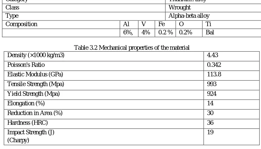
Titanium and its alloys are used extensively in aerospace, such as jet engine and airframe components, because of their excellent combination of high specific strength and their exceptional resistance to corrosion at elevated temperature. The machinability of titanium and its alloys is generally considered to be poor owing to several inherent properties of the materials. Poor thermal conductivity, chemically reactivity and low elastic modulus are the common problems. Typical composition limits and the mechanical properties of Titanium Ti-6Al-4V are shown in Table 3.1 and Table 3.2 respectively.

Table 3.1 Composition of the material

Category Titanium Alloy

Class Wrought

Type Alpha-beta alloy

Composition Al V Fe O Ti

6%, 4% 0.2 % 0.2% Bal

Table 3.2 Mechanical properties of the material

Density (×1000 kg/m3) 4.43

Poisson's Ratio 0.342

Elastic Modulus (GPa) 113.8

Tensile Strength (Mpa) 993

Yield Strength (Mpa) 924

Elongation (%) 14

Reduction in Area (%) 30

Hardness (HRC) 36

Impact Strength (J) (Charpy)

19

C. Experimental Setup

For this experiment the whole work has been carried out by Electrochemical Machining set up from ELECHEM TECHNIK, BANGLORE which is having Supply of - 415 v +/- 10%, 3 phase AC, 50 HZ. And consist of three major sub systems which are being discussed in this chapter. The set up consists of three major sub systems:

1) Machining Cell. 2) Control Panel.

3) Electrolyte Circulation.

IV. DESIGNOFEXPERIMENTS

V.TAGUCHIEXPERIMENTALDESIGNANDANALYSIS

Taguchi’s recommends orthogonal array (OA) for laying out of experiments. These OA’s are generalized Graeco-Latin squares. To design an experiment is to select the most suitable OA and to assign the parameters and interaction of interest to the appropriate columns. The use of linear graphs and triangular table suggested by Taguchi makes the assignment of parameters simple. The array forces all experimenters to design almost identical experiments. In the Taguchi method the results of the experiments are analyzed to achieve one or more of the following objectives:

A. To establish the best or the optimum condition for a product or process. B. To estimate the contribution of individual parameters and interactions. C. To estimate the response under the optimum condition.

The optimum condition is identified by studying the main effect of each of the parameters. The main effects indicate the general trends of influence of each parameter

In the experiment, Minitab 16 software for Taguchi design was used. In this study, 3 level design (three factors) with total of 27 numbers of experiments to be conducted and hence the OA L27 was chosen.

VI. DESIGNOFEXPERIMENTINMINITAB

Taguchi method uses orthogonal array for arranging suitable combination of input signals in a Table to give useful value of output responses. Orthogonal arrays are generalized Graeco Latin squares. In a static response experiment MINITAB software provides both static and dynamic response experiment; the quality characteristic of interest has a fixed level. The quality Characteristic operates over a certain range of values in dynamic response experiment and aim of this experiment is to make better the relation between input signal and output response. This design experiment is used to find best combination of input signals or variables setting that can achieve robustness against noise factors. MINITAB software calculates response tables and generates main effects and interaction plot for:--

Table 4.1 Types of design

2-level design 2 to 31 factors

3 level design 2 to 13 factors

4 level design 2 to 5 factors

5 level design 2 to 6 factors

mixed level design 2to 26 factors

VII. S/NRATIO

According to Taguchi method, the S/N ratio is the ratio of Signal to Noise where signal represents the desirable value and noise represents the undesirable value. Taguchi method stresses the importance of studying the response variation using the signal - to - noise (S/N) ratio, resulting in minimization of quality characteristic variation due to uncontrollable parameter. The metal removal rate was considered as the quality characteristic with the concept of "the larger-the-better". The S/N ratio for the larger-the-better is: S/N = -10*log (mean square deviation):

S/N = -10log10 { )}

Where n is the number of measurements in a trial/row, in this case, n=1 and y is the measured value in a run/row. The MRR values measured from the experiments and their corresponding S/N ratio values were calculated. The MRR response table for feed rate flow rate and inter electrode gap was created in integrated manner. Regardless of the category of the performance characteristics, a greater S/N value corresponds to a better performance. Therefore, the optimal level of the machining parameters is the level with the greatest S/N value.

VIII.PROCEDUREOFTHEEXPERIMENT

Before starting, the experiment measured initial weight of the work piece so we can Measure MRR.

TABLE 4.2FACTOR LEVELS FOR TI-6AL-4V

LEVELS FEED RATE

(mm/min)

FLOW RATE (l/min)

ELEC.CONC. (g/l)

1 0.11 0.65 15%

2 0.16 0.75 21%

3 0.21 0.95 26%

TABLE 4.3L27ORTHOGONAL ARRAY

ex no A B C

1 0.11 0.65 15

2 0.11 0.65 21

3 0.11 0.65 27

4 0.11 0.75 15

5 0.11 0.75 21

6 0.11 0.75 27

7 0.11 0.95 15

8 0.11 0.95 21

9 0.11 0.95 27

10 0.16 0.65 15

11 0.16 0.65 21

12 0.16 0.65 27

13 0.16 0.75 15

14 0.16 0.75 21

15 0.16 0.75 27

16 0.16 0.95 15

17 0.16 0.95 21

18 0.16 0.95 27

19 0.21 0.65 15

20 0.21 0.65 21

21 0.21 0.65 27

22 0.21 0.75 15

23 0.21 0.75 21

24 0.21 0.75 27

25 0.21 0.95 15

26 0.21 0.95 21

27 0.21 0.95 27

IX. GREYRELATIONGENERATION

There are three different types of data normalization according to the requirement of Lower the Better (LB), Higher the Better (HB), or Nominal the Best (NB) criteria. The desired quality characteristics for MRR are HB criterion; therefore, the normalization of original sequence of this response was done by using following equation:

) ( min ) ( max ) ( min ) ( ) ( * k y k y k y k y k y i i i i i   

Where yi*(k) was the normalized data, i.e. after grey relational generation, yi(k) was the kth response of the ith experiment, min yi(k) is the smallest value of yi(k) for kth response, and max yi(k) is the largest value of yi(k) for the kth response. Overcut diameter follows the LB criterion. Accordingly, the normalization of this response is done using following equation:

) ( min ) ( max ) ( ) ( max ) ( * k y k y k y k y k y i i i i i   

A. Grey Relation Co-efficient

The grey relation coefficient was calculated as:

max ) ( max min ) (           k k oi i

Where Ɛi (k) is the grey relation coefficient of the ithexperiment fr the kthresponse.Δoi(k)=lly o*(k) – yi *(k)ll, i.eabsolute of the

difference between y o*(k) andyi *(k). y o*(k) is the ideal or reference sequence. Δ max is the largest value ofΔoi(k), Δ min is the

B. Grey Relation Grade

The grey relation grade (Ґi) is calculated by averaging the grey relational coefficients corresponding to each experiment







i

k

n

(

)

1

Where, Q is the total number of response and n is the number of output responses. The grey relational grade Ґi represents the level

of correlation between the reference sequence and the comparability sequence. If higher grey relation grade occurred than the corresponding parameter combination is closer to the optimal setting.

X.EXPERIMENTALRESPONSESANDOPTIMIZATION

MACHINING OF Ti-6Al-4V: Based on the selected process parameters levels, L27 Orthogonal Array was selected as shown in Table no.5.1 and the combinations of machining operations are performed in electrochemical machine. There are nine experiments required to study the electrochemical machining process parameters by using Taguchi L27orthogonal array

TABLE 5.1FACTORS AND LEVELS SELECTED FOR ECM

Factor Process parameter Level 1 Level 2 Level 3

A Feed rate(mm/min) 0.11 0.16 0.21

B Electrolyte flow(lit/min) 0.65 0.75 0.95

C Electrolyte concentration (%) 15 21 27

The level of the variable process parameters selected on the basis of literature review, results of pilot experiments and the set up constraints.

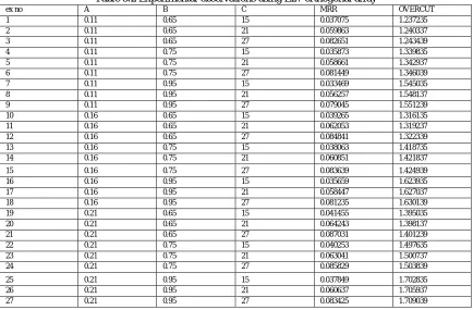
The plan of experiments is made of 27 tests with feed rate, flow rate, electrolyte concentration as input parameters the response to be studied is material removal rate and overcut is exhibited in Table 5.2

Table 5.2 Experimental observations using L27 orthogonal array

ex no A B C MRR OVERCUT

1 0.11 0.65 15 0.037075 1.237235

2 0.11 0.65 21 0.059863 1.240337

3 0.11 0.65 27 0.082651 1.243439

4 0.11 0.75 15 0.035873 1.339835

5 0.11 0.75 21 0.058661 1.342937

6 0.11 0.75 27 0.081449 1.346039

7 0.11 0.95 15 0.033469 1.545035

8 0.11 0.95 21 0.056257 1.548137

9 0.11 0.95 27 0.079045 1.551239

10 0.16 0.65 15 0.039265 1.316135

11 0.16 0.65 21 0.062053 1.319237

12 0.16 0.65 27 0.084841 1.322339

13 0.16 0.75 15 0.038063 1.418735

14 0.16 0.75 21 0.060851 1.421837

15 0.16 0.75 27 0.083639 1.424939

16 0.16 0.95 15 0.035659 1.623935

17 0.16 0.95 21 0.058447 1.627037

18 0.16 0.95 27 0.081235 1.630139

19 0.21 0.65 15 0.041455 1.395035

20 0.21 0.65 21 0.064243 1.398137

21 0.21 0.65 27 0.087031 1.401239

22 0.21 0.75 15 0.040253 1.497635

23 0.21 0.75 21 0.063041 1.500737

24 0.21 0.75 27 0.085829 1.503839

25 0.21 0.95 15 0.037849 1.702835

26 0.21 0.95 21 0.060637 1.705937

The sample calculation for calculating the material removal rate and overcut is shown below. Sample calculation (order 1)

MRR is calculated as given by the following formula:

M .R.R =

(Initial Weight - Final Weight ) =

(53.5 - 52.31)

0.037075g/min

Time (32)

Overcut-diameter is calculated as given by the following formula Over cut diameter = (Observed diameter-Actual diameter) /2= (6.47-4)/2=1.237235mm

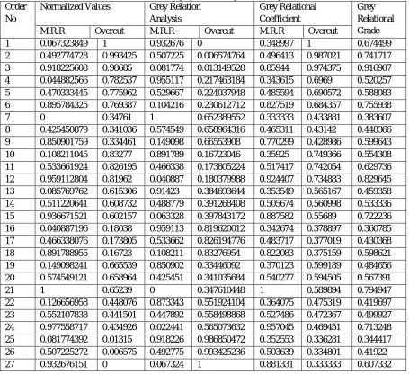
Now, the multiple objective problem has been transformed into a single objective optimization problem using Grey based Taguchi approach. The evaluated grey relation grade for responses shown in Table no 5.3

Table 5.3 Evaluated grey relational grade for responses Order

No

Normalized Values Grey Relation

Analysis

Grey Relational Coefficient

Grey Relational Grade

M.R.R Overcut M.R.R Overcut M.R.R Overcut

1 0.067323849 1 0.932676 0 0.348997 1 0.674499

2 0.492774728 0.993425 0.507225 0.006574764 0.496413 0.987021 0.741717

3 0.918225608 0.98685 0.081774 0.013149528 0.85944 0.974375 0.916907

4 0.044882566 0.782537 0.955117 0.217463184 0.343615 0.6969 0.520257

5 0.470333445 0.775962 0.529667 0.224037948 0.485594 0.690572 0.588083

6 0.895784325 0.769387 0.104216 0.230612712 0.827519 0.684357 0.755938

7 0 0.34761 1 0.652389552 0.333333 0.433881 0.383607

8 0.425450879 0.341036 0.574549 0.658964316 0.465311 0.43142 0.448366

9 0.850901759 0.334461 0.149098 0.66553908 0.770299 0.428986 0.599643

10 0.108211045 0.83277 0.891789 0.16723046 0.35925 0.749366 0.554308

11 0.533661924 0.826195 0.466338 0.173805224 0.517417 0.742054 0.629736

12 0.959112804 0.81962 0.040887 0.180379988 0.924407 0.734883 0.829645

13 0.085769762 0.615306 0.91423 0.384693644 0.353549 0.565167 0.459358

14 0.511220641 0.608732 0.488779 0.391268408 0.505674 0.560998 0.533336

15 0.936671521 0.602157 0.063328 0.397843172 0.887582 0.55689 0.722236

16 0.040887196 0.18038 0.959113 0.819620012 0.342674 0.378897 0.360785

17 0.466338076 0.173805 0.533662 0.826194776 0.483717 0.377019 0.430368

18 0.891788955 0.16723 0.108211 0.83276954 0.822083 0.375159 0.598621

19 0.149098241 0.665539 0.850902 0.33446092 0.370123 0.599189 0.484656

20 0.574549121 0.658964 0.425451 0.341035684 0.540277 0.594505 0.567391

21 1 0.65239 0 0.347610448 1 0.589894 0.794947

22 0.126656958 0.448076 0.873343 0.551924104 0.364075 0.475319 0.419697

23 0.552107838 0.441501 0.447892 0.558498868 0.527486 0.472367 0.499927

24 0.977558717 0.434926 0.022441 0.565073632 0.957045 0.469451 0.713248

25 0.081774392 0.01315 0.918226 0.986850472 0.352553 0.336281 0.344417

26 0.507225272 0.006575 0.492775 0.993425236 0.503639 0.334801 0.41922

27 0.932676151 0 0.067324 1 0.881331 0.333333 0.607332

For getting optimal level parameters the calculation made like as follows Sample Calculation

For Level1 Factor A:

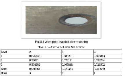
Table no 5.4 shows the Taguchi responses for both material removal rate and overcut and depicts that the optimal factor setting condition is A1B1C3.Feed rate is most influencing factor, after that electrolyte concentration followed by electrolyte flow.

The following photographs taken after the completion of machining process

Fig: 5.1 Work piece snapshot after machining

TABLE 5.4OPTIMUM LEVEL SELECTION

Level A B C

1 0.625446 0.688201 0.466843

2 0.56871 0.57912 0.539794

3 0.538982 0.465818 0.726502

Delta 0.086464 0.222383 0.259659

Rank 3 2 1

For optimal material removal rate and overcut and depicts that the optimal factor setting condition is A1B1C3.Feed rate is most influencing factor, after that electrolyte concentration followed by electrolyte flow

XI.RESULTSANDDISCUSSIONS

In this chapter the effect of process parameter on responses such as MRR and OVERCUT DIAMETERS ARE analyzed

XII.EFFECTONMRR

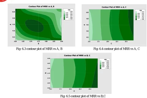
The Fig 6.1 shows the main effects plot for material removal rate increases with increasing in electrolyte concentration mostly, since the current density is proportional to the concentration of electrolyte.

0.21 0.16 0.11 0.09

0.08

0.07

0.06

0.05

0.04

0.90 0.75

0.60 15 21 27

A

M

e

a

n

o

f

M

e

a

n

s

B C

Main Effects Plot for Means

Data Means

0.21 0.16 0.11 -21 -22 -23 -24 -25 -26 -27 -28 -29

0.90 0.75

0.60 15 21 27

A

M

e

a

n

o

f

S

N

r

a

ti

o

s

B C

Main Effects Plot for SN ratios

Data Means

Signal-to-noise: Larger is better

Fig 6.1 Main effect plot for Means Fig: 6.2 Main effects Plot for SN ratio

Also the formation of oxide film on the metal surface hinders efficient ECM and deep grain boundary attack of the metal surface can occur and leads to poor surface finish Material removal rate have the higher

B A 0.90 0.85 0.80 0.75 0.70 0.65 0.60 0.20 0.18 0.16 0.14 0.12 > – – – – < 0.04

0.04 0.05 0.05 0.06 0.06 0.07 0.07 0.08 0.08 MRR

Contour Plot of MRR vs A, B

C A 25.0 22.5 20.0 17.5 15.0 0.20 0.18 0.16 0.14 0.12 > – – – – < 0.04

0.04 0.05 0.05 0.06 0.06 0.07 0.07 0.08 0.08 MRR

Contour Plot of MRR vs A, C

Fig: 6.3 contour plot of MRR vs A, B Fig: 6.4 contour plot of MRR vs A, C

C B 25.0 22.5 20.0 17.5 15.0 0.90 0.85 0.80 0.75 0.70 0.65 0.60 > – – – – < 0.04

0.04 0.05 0.05 0.06 0.06 0.07 0.07 0.08 0.08 MRR

Contour Plot of MRR vs B, C

Fig: 6.5 contour plot of MRR vs B,C

In the above figure6.3 ,6.4, 6.5 show the variation of MMR with respect to Feed rate (mm/min) Electrolyte flow (lit/min) and Electrolyte concentration (%).the dark green show the higher MRR zone and its better for optimum machining

0.20 0.04 5 1 . 0 0.06 5 1 8 0 . 0 20 0.10 5 2 R R M A C C , A s v R R M f o t o l P e c a f r u S

Fig: 6.6 surface plot of MRR vs A, C

Fig 6.6 show the surface plot of MRR with respect to factor A and C. its plane variation with factor C is high as compare to factor A . Statistical tool which, based on the experimental values, will help to infer some important conclusions. The level of significance or the influence of a factor on a particular output response could be revealed by this method. The conventional way of looking into the averages of results to know the desirable factor levels doesn’t account the variability of results within the trials..

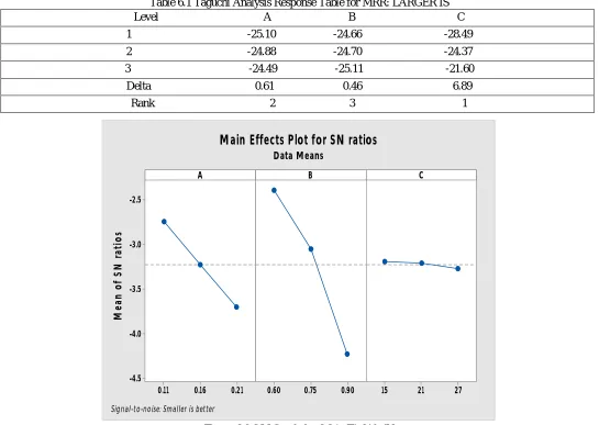
For higher productivity, a higher material removal rate is always desired; hence, MRR has been categorized as ‘larger-the-better’ type problem. The signal-to-noise ratio in this case has been calculated as follows:

S/N of MRR = -10log10 (square reciprocal of MRR)

Table 6.1 shows Taguchi analysis response for material removal rate. In summary, the optimal combination level of the machining parameters is A3B1C3.ie, (Exp. No.21) with feed rate 0.21 mm/min, flow rate of 0.60 lit/min and Electrolyte conc. of 27%.

Table 6.1 Taguchi Analysis Response Table for MRR: LARGER IS Level A B C

1 -25.10 -24.66 -28.49 2 -24.88 -24.70 -24.37

3 -24.49 -25.11 -21.60

Delta 0.61 0.46 6.89 Rank 2 3 1

0.21 0.16 0.11

-2.5

-3.0

-3.5

-4.0

-4.5

0.90 0.75

0.60 15 21 27

A

M

e

a

n

o

f

S

N

r

a

ti

o

s

B C

Main Effects Plot for SN ratios

Data Means

Signal-to-noise: Smaller is better

Figure 6.8 S/N Graph for OC in Ti-6Al-4V

XIII.CONFIRMATIONTEST

The experimental confirmation test is the final step in verifying the results drawn based on Taguchi’s design approach. The optimal conditions are set for the significant factors and a selected number of experiments are run under specified cutting conditions. The average of the results from the confirmation experiment is compared with the predicted average based on the parameters and levels tested. The confirmation experiment is a crucial step and is highly recommended by Taguchi to verify the experimental results. In this study, a confirmation experiment was conducted by utilizing the levels of the optimal process parameters (A1B1C3) for metal removal rate and overcut in the electrochemical machining of Titanium Ti-6Al-4V and obtained as 0.083551 g/min and 1.23372 mm respectively.

XIV. CONCLUSION

Experimental works were done on Ti-6Al-4V material by using Taguchi L9 orthogonal array. By using S/N ratio analysis we found the optimum level for each factor that would lead us to optimum machining condition to obtain an optimum level in achieving high material removal rate, minimize OC-diameter. The following conclusions are arrived.

REFERENCES

[1] J.A. McGeough( 1974)Principle of Electrochemical Machining, Chapman and Hall, London H. El-hofy (2007) Fundamentals of Machining Processes, Conventional and Non - conventional Processes, Taylor & Francis Group

[2] Strode and M. B. Bassett(2008) The effect of Electrochemical Machining on the Surface Integrity and Mechanical Properties of Cast AND Wrought Steels, Wear, 109,171- 180.

[3] H. Hocheng, P.S. Pa(2010)The application of a turning tool as the electrode inelectropolishing, Journal of Materials Processing Technology 120,6-12. [4] D. Zhu, K. Wang, J.M. Yang(2010)Design of Electrode Profile in Electrochemical Manufacturing Process, CIRP Annals-Manufacturing Technology 52,

169-172.

[5] K.P. Rajurkar, D. Zhu, B. Wei(2007) Minimization of Machining Allowance inElectrochemical Machining, Annals of the CIRP Vol. 47165-168.

[6] Jinhua Zhu and Baocheng Wang(2007) Effect of electrochemical polishing time onsurface topography of mild steel, Journal of University of Science and Technology 14236-239.

[7] C.S.Chang, L.W.Hourng,C.T.Chung(2009)Tool design in electrochemicalmachining considering the effect of thermal-fluid properties, Journal of AppliedElectrochemistry, 29, 321-330.

[8] The maximum material removal rate is obtained as 0.082651 g/min and overcut as 1.243439 mm by optimum machining condition.

[9] From the grey relation grade the optimal machining parameter settings are obtained for Ti6Al4V is feed 0.11mm/min, 0.60lit/min and electrolyte concentration 27%.