Finite Time Engineering
Subhendu Das
Abstract – All microprocessor based electronic systems are designed as repetition of finite time activities. The classical infinite Laplace transform (ILT) theory violates this fundamental requirement of engineering systems. We show that this theory assumes that all signals must exist over the entire infinite time interval. Since in engineering this infinite time assumption is not meaningful, this paper presents a modeling, analysis, and design approach for linear time invariant systems using the theory of the finite Laplace transform (FLT).
Index Terms – Convolution, finiteLaplace transforms, linear systems, numerical inversion.
I. INTRODUCTION.
Most of our engineering systems run over finite time. Consider the example of a robotic arm, picking up an item from one place and dropping it in another place and repeating the process in, say, less than a second of time. Similarly a digital communication receiver system, receives an electrical signal of microsecond duration, for example, representing the data, extracts the data from the signal, sends it to the output, and then goes back to repeat the process.
Our software runs under operating systems (OS) which are also nothing but finite state machines. A finite state machine is a collection finite number of activities of finite durations, repeated asynchronously and/or synchronously based on the external as well as internal events. The signals and the environment are changing every OS time slice. This is the general nature [1] of our technology today.
In most applications if we examine any internal data of the microprocessor using say, JTAG emulators, and plot its numerical values over time, the graph will look like a stochastic process. There is no steady state at nanosecond time scale and 16 or 32 bits data resolution. As an example see the Kalman Filter state variable estimate of the position of a GPS receiver as shown in the Figure 17 of [2]. The data in that graph is shown at the time resolution of seconds and still looks like a random function. Our engineering systems show steady state results only after filtering, averaging, and then displaying at time resolution of the order of seconds.
The classical Laplace transform theory violates the requirements of modern engineering implementations. (a) We show that the ILT is valid only for infinite duration signals. On the other hand the modern engineering uses finite duration signals. (b) ILT models have poles; the FLT models do not generate poles. Thus ILT models may introduce instability in engineering implementations. (c) ILT requires convolution which is not valid for finite duration signals. (d) ILT methods are based on steady state concepts. Microprocessors do not see steady state in engineering implementations. (e) Infinite time theory for
finite time engineering forces us to introduce software patches and kludges to make it work.
II. THE FINITE LAPLACE TRANSFORM
The Laplace transform is defined as [3]:
= ∞
(1)
Since the upper limit is infinity, this definition will be referred to as the ILT. This infinite limit requires a boundedness condition for (1) given by:
|| ≤ , 0 < <∞ (2)
It can be shown [3, p. 13] that (1) converges for all ℛ >
. This region is called the region of convergence. Here
ℛ means the real part of the complex variable s. We briefly present some basic theories [4] of the FLT.
The FLT is defined as [4, pp 283-294]:
ℒ = = , 0 < <∞ (3)
We will use F(s) to denote the FLT of a continuous function
f(t). In (3) t will be referred to as time, [0,T] as finite duration interval, s as a complex variable represented by
x+iy, where x and y are real variables. Since the upper limit is finite, the integral (3) always exist. Unlike the ILT, the region of convergence of FLT is the entire complex plane.
An example of the FLT [4] will show that the ILT is based on infinite time assumptions. Define the step function:
= 1 0 ≤ ≤ 0 !ℎ#$%& (4) Using the definition (3) we get the expression for the FLT:
ℒ1 = . 1. (5)
=(−( (6)
=(*+,- (7)
We can see from (6) that the FLT has the ILT term ( and an expression involving . This exponential term will always be there in all the FLT expressions. As T goes to infinity this exponential term will go to zero.
The expression (6) will become ILT, only if the second part of (6) is zero, which in turn means T is infinity. From (5) we see that even if the integration limit is infinity, the definition (4) will keep the second part in (6). Thus (6) will become ILT only when the function f(t) is nonzero over the entire infinite interval. Thus whenever we are using the ILT, we are assuming that the signals exist for infinite time.
It is also worth noting at this time that (7) does not have a pole at s=0, because the numerator goes to zero as s
approaches zero. This property of 0/0 indeterminate form, is a very distinguishing feature of the FLT. For later references we also record the FLT pairs [4].
.↔(*
. (8)
sin $ ↔ 4
5645− 5644 5cos $ − 5645sin $ (9)
cos $ ↔
5645− 5645cos $ + 5644 5sin $ (10) Manuscript received July 24, 2011; Revised August 16, 2011. The author
From the fundamental theorem of calculus [5, p. 142] we know that if f(t) is continuous on [a,b] and F(t) is the antiderivative or integral of f(t) defined by
= then = : − ;.<
In the above fundamental theorem if we define
, = then it is clear that
FLT: , − , 0 (11)
ILT: −, 0 (12)
It is easily seen from (11) and (12) that the ILT has been defined in such a way that F(s,∞) is zero and we only have – F(s,0) in (12), the part that we always get in the FLT.
It seems that the FLT theory was first introduced by Dunn [6]. Later another paper was published by Debnath [7], which is also available as a chapter in the book by Debnath [4]. The objectives of both papers were to extend the ILT theory to cover a larger class of Laplace transformable functions. The motivation of this paper is driven by the finite time requirement [8, pp. 73-88] of engineering.
III. THE FLTPROPERTIES
In this section we discuss some of the important properties of the FLT theory relevant to system engineering.
A. Analyticity
The proof of analyticity is not given in [4] or [6] or in any other places as far as we know. Yamamoto [9] points to the Paley-Wiener theorem for the proof. A function F(s) of complex variable s is analytic at a point s0 if F(s) has a
derivative in some neighborhood of s0. A function F(s) is
called an entire function if it has derivatives at each nonzero point in the finite complex plane [5, p. 73].
Theorem: The complex FLT function F(s) satisfies the
following conditions:
(a) = =>, ? + %@>, ? is defined over the entire complex plane,
(b) The first order partial derivatives of u and v exist at all points s=x+iy in the plane, and
(c) The partial derivatives are continuous and satisfy the Cauchy-Riemann equations
=A= @B , =B= −@A , at all points in the plane. Therefore ′
exists at all points in the complex plane and
F(s) is an entire function.
The proof follows the lines of the ILT similar to [3, pp. 124-125]. For any s=x+iy in the finite plane we can write:
= = A6CB
= A
cos ? + % Asin ?
= =>, ? + %@>, ? (13)
It is clear from (13) that u and v are well defined and exist since the functions are continuous and the integration is over finite duration. Also,
=A=DAD E Acos ? F =
DADAcos ?
(14)
The partial derivative in (14) can be moved from outside the integral to inside because of finite duration and the continuity of all functions involved. Thus unlike in the ILT
case there are no absolute or uniform convergence issues to be considered. Hence we can write from the last expression
=A= DAD Acos ?
= − Acos ?
(15)
Similarly we can show that
@B= DBD −Asin ? =
− Acos ?
(16)
The above two expressions, (15) and (16), show that
=A= @B . Similarly we can also show that =B= −@A . These equality conditions on partial derivatives, called Cauchy-Riemann conditions [5, p. 66], indicate that the derivative of
F(s) exists for all s in the entire plane and thus by definition
F(s) is an entire function. ■
The proof of the Paley Weiner theorem can be found in Rudin [10, pp. 180-185].
B. Taylor Series
One of the fascinating properties of functions of complex variables is that if it is analytic then it has all the derivatives. Thus F(s) has the Taylor series expansion around the origin and is valid over the entire complex plane [5, pp. 189-192].
= ∑∞ HIJ!
JL J (17)
Therefore F(s) can be approximately expressed by:
≈ ;+ ;((+ ;NN+ ⋯ + ;PP (18) Interestingly the expression (17) is not valid for the ILT.
C. The FIR Filter
A Finite Impulse Response (FIR) filter uses the sampled values of the continuous time input signal and is defined as a linear combination of present and previous values of the input signal. A FIR filter is defined as [9, 11, pp. 148-158]:
QR = ∑P(ℎS RT
TL (19)
Here H(z) is the transfer function of the FIR filter, z is the variable for the Z-Transform, and h(k) is the k-th time sample of the impulse response of the continuous time signal. Thus H(z) is a polynomial in z and has no poles in the Z-plane. The FLT shares these two properties with the FIR filter. It is worth noting also that the expressions (18) and (19) are very similar. We can say that the FLT is the continuous time equivalent of the discrete time FIR filter.
D. Stability
The stability concept is related to the behavior of a function f(t) as t approaches infinity. Since in engineering infinite time is not meaningful, the usual stability concept is also not meaningful. The final value theorem lim→∞ =
lim → is not applicable in finite time engineering.
Moreover as FLT does not have poles, the corresponding time function cannot go to infinity.
A microprocessor never sees a steady state function. In every OS time slice T, the signals are changing. The signals in communication systems may change at rates faster than T. Thus the steady state ILT concept does not exist in the engineering systems. The FLT systems can be used the way we use the FIR filter problems.
related to the ILT, associated poles, infinite time, and are not meaningful for the FLT and in modern engineering.
E. The Inverse FLT
For the ILT theory the inverse is defined by the following relation [3, pp. 152-157]:
=NXC( A6C∞
AC∞ (20)
Here x > α, and α is defined in (2). It can be shown that (20)
is equivalent to the following contour integral:
=NXC( Y Z (21)
Here the contour C is taken appropriately to cover all the singularities on the left of the vertical line, called Bromwich line, passing through the point α. Normally (21) is computed
using the relation
(
NXCY Z = ∑PTL(lim W[\ ) RT (22)
Here zk is a pole of F(s). The approach based on (22) is
known as the residue method. Since the FLT does not have any poles, the method in (22) cannot be used to find the inverse of the FLT functions.
Thus one of the very useful methods for the ILT is no longer valid for the FLT. However, as mentioned before, many authors [6, 7] have treated the two terms in expression (11) separately using separate contours. In the following section we present a numerical method for the inversion of the FLT that uses the analyticity property of the combined expression (11).
IV. NUMERICAL INVERSION
Probably Bellman was the first person to introduce the numerical approach concept in Laplace transform theory. Bellman [13, pp. 135-155] uses positive real integers for s
before integrating the ILT equation (1) as real and imaginary integrals. [14], [15] give a summary of recent most popular numerical methods, including Post-Widder and Talbot’s methods. Numerical inversion of the ILT is also an ill-posed problem as pointed out in [16].
We present here a numerical inversion method that takes advantage of the analyticity property of the FLT functions. This approach is unique to the FLT; however it has some similarity with the FIR filter methods. The objective is to find the time function f(t) from the known FLT function
F(s). Since F(s) is analytic, it has the Taylor series:
;9 ;( 9 ;NN9 ;]]O (23)
Expanding the exponential function under the integral sign, ( is an analytic function), and equating the like powers of s in (23) it can be shown that
;J )1J (J! J (24)
Thus the problem reduces to finding f(t) in (24) given all the coefficients ^;J, _ 0,1, O , `a. We expand f(t) in Taylor series, assuming that f(t) has all the derivatives, which may not be practical even in engineering.
:9 :( 9 :NN9 :]]O (25)
We can now substitute (25) in (24) and express each coefficient an in terms of bn for n=1…N, to get
;J ∑PTL()1J (J!J6T6(( J6T6(:T (26)
For N=4, as an example, using matrix notation we can express equation (26) in a more readable form as in (27). We can now solve the matrix equation (27) by inverting the square matrix to find the b-coefficients {bk}. Clearly, the
matrix is non-singular, because the columns are independent. These b-coefficients can then be used in (25) to find the function f(t).
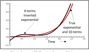
As an example consider the FLT expression (8) for the exponential function. The inverse was generated using the Mathematica analysis tool. The Fig.1 shows how the inverse compares with the exact exponential function with four coefficients of the FLT Taylor series (23). For 10 FLT coefficients, the true graph and the numerically reconstructed graph match exactly at the resolution of the paper. The numerical data are shown in the Table 1. The Taylor series based approach appears to be very robust and satisfactory even for small number of terms. This does not normally happen for FIR filters.
The Taylor series approach has been used [17] for the ILT inversion analytically. Their approach expands the function
f(t) in Taylor series and evaluates over discrete values of s. In our paper we have expanded all functions, f(t), F(s), and
e-st over all s. Also our approach is a numerical approach for the FLT.
;0 2
2
3 3
4 4
:0
;1 )2
2 )
3
3 )
4
4 )
5 5
:1
;2 1
2! 3
3 1 2!
4 4
1 2!
5 5
1 2!
6 6
:2
;3
)3!144 )3!155 )3!166 )3!177 :3
= (27)
True exponential data samples
0.00451658 0.00822975 0.0149956 0.0273237 0.0497871 0.090718 0.165299 0.301194 0.548812 1.0
Exponential from inverse FLT with four coefficients
0.0133275 0.030779 0.0271752 0.0214159 0.0324014 0.0790315 0.180206 0.354826 0.621791 1.0
Exponential from inverse FLT with ten coefficients
[image:3.612.87.272.51.159.2]0.00451518 0.00823095 0.0149953 0.0273231 0.0497887 0.090718 0.165299 0.301198 0.548813 1.0
Table 1: Numerical inversion of FLT
0.5 1.0 1.5 2.0 2.5 3.0
-0.1 0.0 0.1 0.2 0.3 0.4
4-terms Inverted exponential
True exponential and 10-terms
Time
[image:3.612.320.539.383.483.2]V. APPLICATIONS
Many standard results of the ILT can be extended in a straight forward way using the methods shown in [3] to the case of the FLT. We only present some results that will be required for our main objective and are not available in the literature. Consider the FLT of the first derivative:
ℒ[′] ′
& | 9
) 0 + (28)
It shows that a first order differential equation (DE) will lead to a two point boundary value problem. Note that f(T)
in (29) is not known because it depends on the solution. The other two terms in (28) are same as in the ILT.
Using an example we illustrate how the boundary conditions can be determined to solve a DE. Consider a second order simultaneous DE taken from [3, p. 65]:
hB
h= −R, h[
h= ?, ?0 = 1, R0 = 0
Taking the FLT on both sides results
i − ?0 + ? = −j
j − R0 + R = i
Solving them we get
i = 56(− 56(? + (56(R (29)
j = 5(6(− 5(6( ? − 56( R (30) From the expression for Y(s) in (29) we get
i = 5(6( − ? + R (31)
Since the denominator of (31) is zero at ± i, the numerator of (31) also should be zero at these values to make Y(s)
analytic at all points in the s-plane. Therefore we must have, from (31),
− ? + R = 0, ; = ±%
Substituting these values of s in the above expression we get the following two equations
%C− %? + R = 0 ; −%C+ %? + R = 0
Solving them simultaneously gives ? = cos , and
R = sin . These boundary conditions in (29) and (30) will help to select the correct solution using (9) and (10).
VI. CONVOLUTION THEOREM
Surprisingly, the FLT literatures [4],[6],[7] do not talk about the convolution theorem. This property says that if the impulse response of a linear time invariant (LTI) system is given by h(t) then the response y(t) for any other input u(t)
can be obtained by the following convolution integral:
? = =m ℎ − mm (32)
It is worth pointing out here that h(t) exists for infinite time and therefore y(t) is also defined for infinite time, independent of the duration for u(t). Using the convolution theorem for the ILT [3, p. 92], (32) can be reduced to
i = Q. n (33)
The ILT convolution theorem can help us to cascade systems to find the combined output from the input U(s):
i = i(QN = nQ(QN (34)
In (34) H1 and H2 are two boxes connected in series and Y1 is the output of the first box.
We illustrate with an example that the ILT convolution theorem cannot be valid for the FLT systems. The idea is very basic and can be found in many engineering text books,
for example [18, pp. 63-75]. We normally overlook the point that is important for the FLT, so we present it in details. Consider the functions defined below:
= Q. − , 0 ≤ ≤ (35)
o = Q< − , 0 ≤ ≤ (36)
Here H(t) is the Heaviside step function defined by
Q = 1, ≥ 00, < 0&
They are same as (4) only with different notations. The convolution of these two functions gives:
ℎ = mo − mm
= Q . − mQ< − − mm
= Q . − mQ< − + mm (37) It is easy to visualize from (37) that h(t) is a triangle with duration 2T. Thus (37) extends beyond the domain of definition of the two functions involved. Because of this reason if we consider the FLT for only time T, a portion of
h(t) will not be considered in the FLT, and the convolution theorem will not work. This will not be apparent from the proof of the theorems for both the ILT and the FLT, because both proofs follow almost exactly the same statements as shown below. A closer look will show that the theorem works for the ILT because the ILT assumes infinite time.
Theorem: If f and g are continuous on 0, then the
FLT relation given below is true:
ℒ. ℒo ≠ ℒ ∗ o (38)
The theorem is proved in the following way [3, pp. 91-93]. Using the definition of the FLT (3) we write
ℒ. ℒo = E s@@F E to==F (39)
Since all functions are continuous in the square region bounded by 0 ≤ = ≤ ;_ 0 ≤ @ ≤ we can move the second integral sign in (39) at the left to get
= E t6s
@o==F @
(40)
Now we define u+v=t and change the limits of the second integral in (40) as shown below
= E s6s @o − @F @ (41)
Since the function f(t) is zero for t > T, we can change the upper limit from T+v to T. If t<v the function g(t-v) is zero, so we can set the lower limit v to zero also, without affecting the integral and can write:
= E @o − @F @ (42)
Again switching the order of integration in (42) we get
= E @o − @@F (43)
Now take the exponential outside the inner integral of (43), because the variable of integration is v inside and write:
= E @o − @@ F (44)
Since v cannot be greater than t for the function g(t-v) is zero in that region, therefore the upper limit T for v can be set to t, giving us.
= E @o − @@ F (45)
Now we have the convolution expression inside (45). We know that the convolution integral in (45) goes beyond T
(45) is 0 to T, and therefore (45) cannot be equal to (46) given below:
ℒ ∗ o (46)
This concludes the proof of the convolution theorem for the FLT system. ■
The reason that the convolution theorem holds in the ILT expressions, is because the ILT expressions are by definition valid only for infinite time, as can be seen from (11) and (12). Thus we cannot multiply two FLT transfer functions, like in (34). In the following section we show how we can go around the lack of a convolution theorem and still use the FLT theory to design engineering systems.
VII. SYSTEM DESIGN
The core idea behind the ILT approach can be described with the help of the standard block diagram shown in Fig.2. In this figure all variables represent the ILT functions. The objective of the design is to find the parameters of the controller C(s) so that the error e(t), the inverse ILT of E(s), meets the engineering requirements.
Ideally, of course C(s) could be selected as the inverse of
P(s) [19, p. 24] but for many reasons that cannot be done. However, in the absence of a convolution theorem, and finite time constraints, that concept is also not meaningful any more. In this section we illustrate the basic idea of the FLT based design method using an open loop system and a simple differential equations (DE). We will see later that the close loop extension is quite trivial. The objective is to demonstrate that the ILT based trial and error method can be extended to the FLT theory. Consider the plant model:
uJh
IB
hI9 uJ(h
I+vB
hI+v9 O 9 u(hBh9 u? = (47)
The FLT of n-th order derivative can be written as
ℒw?Jx Jℒ[?] ) ∑J(TLT?JT(0 +
∑J(T
TL ?JT(
We use the following simplifying notation
?J0, = − ∑J(TLT?JT(0 + ∑J(TLT?JT(
Using the above notation FLT of (47) can be written as uJJi + uJ?J0, + uJ(J(i + uJ(?J(0, +
⋯ + u((i + u(?(0, + ui = n
Using more simplifying notations the last expression can be reduced to
yJi + yJ0, = n (48)
In (48) we have borrowed the notation style from the software engineering concepts, that is
yJ = ∑JTLuTT and yJ0, = ∑JTLuT?T0, Therefore from (48) we can express Y(s) of the plant as:
i =z(
I n − zI,
zI (49)
Similarly the controller model C(s) can be written as:
n =Z(
{ | −
Z{,
Z{ (50)
Even if the initial conditions are zero the right hand side of (49) will still be non-zero, because it includes the final time values. This is also another reason, besides the lack of
the convolution theorem, why we cannot multiply two transfer functions in the FLT based systems.
The block diagram in Fig.3 shows the composite open loop system. The design objective is to find the unknown coefficients of the controller Cm(s), for the known plant and
the known reference input. Since we cannot multiply the two blocks together we must consider the output of the individual blocks separately and then feed them to the following blocks as shown in Fig.3.
A. Design Example
The following example and its numerical simulation will illustrate the details. Consider a first order known plant:
?} + u? = =, 0 ≤ ≤ (51) Here u(t) is the output from the controller and is also the input to the plant, and p is a plant parameter of known value. Assume also a first order controller with unknown controller parameter c and a known input r(t) as in (52):
=} + ~= = # = 1 , 0 ≤ ≤ (52)
For simplicity all initial conditions are assumed to be zero. The FLT of the controller (52) gives
n + = + ~n =(*+,-
n = 6( (*+,-−*+,- 6t
=(*+,- 6 *+,-t (53)
Since U(s) must be analytic we have, from (53), at s=-c,
1 − + ~= = 0
This gives the boundary value for u(T) as
= =(*+- (54)
The FLT of the plant (51) gives:
i + ? + ui = n
Solving for Y(s) we can write
i = 6( n −*+,- 6B
We can now substitute for the input U(s) from (53) to get
i = 6( (*+,- 6 *+,-t−*+,- 6B
=(*+,- *+,- 6 6t 6*+,-B (55) Again using analyticity of Y(s) at s=-p, we get from (55):
1 − + u= + u~ − u? = 0
This produces the the terminal value of y(T) as
? =(*+-t (56)
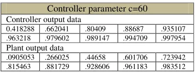
We have assumed p=50 for the plant. First we try c=60 and find u(T) and y(T) using (54) and (56). Then we find the input to the plant by inverting the controller FLT (53) using Taylor series method. Finally we invert the plant (55), again using Taylor series, to find the output from the plant. The process can be repeated with another trail value for c. The results are shown in Fig.4 and Table 2.
Fig.2: A control system design approach
P(s) C(s)
R(s)
Y(s) E(s)
+
-
n = | −1 0,
i =yJ n −1 yJ0,yJ Y(s) U(s)
R(s) U(s
)
The signals can be added or subtracted at all points, including the feedback points, since the FLT is a linear operation, and because we are considering only linear systems. Thus it is clear from the above design principle that the method can be easily extended for the design and analysis of various standard problems in engineering like: close loop system design, parameter sensitivity analysis, transient characteristics etc.
The first paper on the application of the FLT to control systems was presented by Datko [20]. Using the analyticity property of the FLT he has shown how the optimal value for the final time can be computed. He has also used the FLT theory for quadratic optimal control problem to find the terminal conditions. [9] uses a sequence of the FLT to generate the ILT to analyze tracking control problem. Rosen [21] has assumed the control law as a linear combination of exponential functions of the FLT variables between two sample intervals. In our paper we have shown how the classical ILT based concepts can be extended to find continuously varying control functions using the FLT.
VIII. CONCLUSIONS
We examined the effect of changing the infinite time requirement for the Laplace transform theory on engineering applications. The most important feature of the Finite Laplace transform (FLT) theory is that they do not introduce any poles. Thus it eliminates all stability problems just like the FIR filters. It is shown that the FLT does not satisfy the convolution theorem. We have given a simple numerical method for the inverse FLT, which helps to design finite time engineering problems.
ACKNOWLEDGEMENTS
The author is deeply indebted to Professor Joel L. Schiff of Mathematics department, University of Auckland, New Zealand, for many help he has provided so gracefully and quickly during the early development of this research work. The author is thankful to him for reviewing the first version of the original paper. The author also remembers that this problem was first discussed with Professor Kalyan Ray of
electrical engineering department of Jadavpur University, Calcutta, India, when we were graduate students.
REFERENCES
[1] S. Das, N. Mohanty, and A. Singh, “Function modulation - the theory for green modem”, Int. J. Adv. Net. Serv.,Vol.2, No. 2&3, pp.121-143, 2009.
[2] M. Nylund, B. Alison, and J. J. Clark, “Kinematic GPS-Inertial navigation on a tactical fighter”, Proc. ION GPS, Portland, 2003 [3] J. L. Schiff, The Laplace transform, theory and applications,
Springer, NY, 1999.
[4] L. Debnath, Integral transforms and their applications, CRC press, 1995.
[5] J. W. Brown and R. V. Churchill, Complex variables and applications, eighth edition, McGraw Hill, NY, USA, 2009. [6] Dunn, H.S. “A generalization of Laplace transform”, Proc. Cambridge
Philos. Soc., 63, pp. 155-161, 1967.
[7] Debnath, L. and Thomas, J., “On finite Laplace transforms with applications”, Z. Angew. Math. Und Mech, 56, pp. 559-563, 1976. [8] P. A. Laplante, Real-time systems design and analysis, Third Edition,
IEEE Press, New Jersey, 2004
[9] Y. Yamamoto, “A function space approach to sampled data control system and tracking problems”, IEEE Tran.AC., Vol. 39, No. 4, April 1994.
[10] W. Rudin, Functional analysis, McGraw Hill, NY, 1973.
[11] P. S. R. Diniz, E. A. B. Da Silva, and S. L. Nitto, Digital signal processing, systems analysis and Design, Cambridge Uni. Press, UK, 2002.
[12] G. F. Franklin, J. D. Powel, and A. E. Naeini, Feedback control of dynamic systems, Prentice Hall, sixth edition, 2009.
[13] R. E. Bellman and R. S. Roth, The Laplace transform, World scientific, Singapore, 1984.
[14] P. O. Kano, M. Brio, J. V. Moloney, “Application of weeks method for the numerical inversion of the Laplace transform to the matrix exponential”, Comm. Math. Sci, Vol. 3, No. 3, pp. 335-372, 2005. [15] G. V. Milovanovic and A. S. Cvetkovic, “Numerical inversion of the
Laplace transform”, Ser. Elec. Energ., vol. 18, No. 3, pp. 515-530, December 2005.
[16] M. Iqbal, “Classroom note, Fourier method for Laplace transform inversion”, J. App. Math & Dec. Sci, 5(3), pp. 193-200, 2001. [17] H. Y. Chung and Y. Y. Sun, “Taylor series approach to functional
approximation for inverse Laplace transforms”, Electronics Letters, Vol. 22, No. 23, 1986.
[18] M.J.Roberts, Signals and systems, Analysis using transform methods and Matlab, McGraw Hill, NY, 2004.
[19] S. Skogestad and I. Postlethwaite, Multivariable feedback control, analysis and design, Second edition, Wiley, England, 2005. [20] Datko, R., “Applications of finite laplace transform to linear control
problems”, SIAM J. of Cont. Optim., Vol. 18, Issue 1, pp. 1-20, Jan 1980.
[21] O. Rosen, Imanudin, and R. Luus, “Final-state sensitivity for time-optimal control problems”, Int. J. Control, Vol. 45, No. 4, pp. 1371-1381, 1987.
[22] R. Priemer, Introductory signal processing, World scientific, Singapore, 1991.
[23] Y. Eideman, V. Milman, A. Tsolomitis, Functional analysis, an introduction, Amer. Math. Soc, Providence, Rhode Island, 2004.
0.02 0.04 0.06 0.08 0.1
[image:6.612.87.281.53.172.2]0.2 0.4 0.6 0.8 1
Fig. 4: Response graphs for controller c=60
Plant response
Controller response
Controller parameter c=60
Controller output data
0.418288 .662041 .80409 .88687 .935107 .963218 .979602 .989147 .994709 .997954
Plant output data
.0905053 .266025 .44658 .601706 .723942 .815463 .881729 .928606 .961183 .983512
[image:6.612.87.281.436.509.2]