Abstract—The flow of a stream coming out of a pipe and hitting a horizontal wall is considered. Both cases of rising and falling flows are studied. First, for the rising flow, depending on the length of the wall L and the Froude number F, the wall can either divert the stream or lead to its detachment. The problem is reformulated using conformal mappings and the resulting problem is then solved by a collocation Galerkin method. A particular form is assumed for the solution, satisfying Bernoulli’s equation on the free surfaces at certain discrete points. The resulting equations are solved by Newton’s method. Solution profiles are presented for particular values of F and the question of the lift exerted on the wall is addressed. Then, the falling flow case is studied in the presence of a horizontal wall of infinite length. Depending on the elevation H of the pipe relative to the horizontal wall and F, the flow can either leave the pipe tangentially or detach from the edge of the pipe. Results are presented showing either a tangential departure from the pipe and no squeezing, or a tangential departure from the pipe followed by squeezing of the liquid. Finally, the cases of flows in the presence of stagnation points are discussed.
Index Terms—free-surface flow, impact, jet, stagnation.
I. INTRODUCTION
In general, the numerical computation of free-surface flows in the presence of gravity is a notoriously difficult problem. One important case of such flows is the case of rising and falling flows. Rising flows occur in numerous applications, as steady jets rising and falling under gravity (see, for example, [1]), water fountains [2], bow flows with a jet in front of the ship [3], flows emerging from a nozzle and falling under gravity [4]–[5]. On the other hand, the problem of falling flows finds applications in such problems as jets falling from nozzles and funnels [6]–[7], rising bubbles [8]–[10], bubbles rising in an inclined pipe [11]–[12], the emptying or the filling of a closed pipe and surf-skimmer planing hydrodynamics [13]–[15]. For more related studies see [16]–[17].
The present paper, which is basically a review of [16]–[17], gives insight to two realistic cases: (i) the case where a wall
Manuscript received March 4, 2010. This work has been supported by ANR HEXECO, Project no BLAN07-1_192661 and by the 2008 Framework Program for Research, Technological development and Innovation of the Cyprus Research Promotion Foundation under the Project AΣTI/0308(BE)/05.
Paul Christodoulides is with the Faculty of Engineering and Technology, Cyprus University of Technology, Cyprus (corresponding author, phone: +357 25002611; fax: +357-25002635; e-mail: paul.christodoulides@ cut.ac.cy).
Frédéric Dias is with the School of Mathematical Sciences, University College Dublin, Ireland, on leave from CMLA, Ecole Normale Supérieure de Cachan and CNRS, France (e-mail: [email protected]).
Lazaros Lazari is with the Department of Mechanical Engineering, Higher Technical Institute, Cyprus (e-mail: [email protected]).
diverts the jet emerging from a pipe pointing upward, and (ii) the case where an infinite wall diverts the jet falling from a pipe pointing downward. Several limiting cases are discussed as well.
When a stream of fluid flows up and out of the top of a long two-dimensional vertically-sided pipe of width 2W and meets a horizontal wall of length 2L set at a height H above the top of the pipe, the flow splits into two jets that reach a maximum height on each side of the wall and then fall under gravity. The solution depends on H/W, L/W and on the dimensionless Froude number
, gW U
F (1)
where g is the acceleration due to gravity and U the velocity of the fluid far inside the pipe.
The problem is formulated in §II. Conformal mappings lead to a formulation of the problem that is well-suited for discretization. A system of N nonlinear equations in N
unknowns is then derived and is solved numerically through a collocation Galerkin method explained in §III, where the numerical results and computed profiles of the free surfaces are presented as well. A study of the lift force exerted on the horizontal wall and of the pressure distribution along the wall is performed in §IV.
Then, based on a similar formulation, we consider a stream of fluid flowing down and out of the bottom of a long two-dimensional vertically-sided pipe of width 2W. The downwardly directed flow meets a horizontal wall of infinite extent set at a distance H below the bottom end of the pipe. The flow splits into two jets on each side of the pipe following a path along the horizontal wall. Again, the solution of the problem depends on the ratio H/W and on the Froude number F. The numerical results of computed profiles and a study of the pressure along the horizontal wall are presented in §V.
Finally, in §VI we study related flows, where the detachment point along the wall is a stagnation point.
II. RISING STREAMS:FORMULATION OF THE PROBLEM We consider the steady irrotational flow of an incompressible inviscid fluid emerging from a pipe of width 2W directed upward, hitting a horizontal wall of length 2L
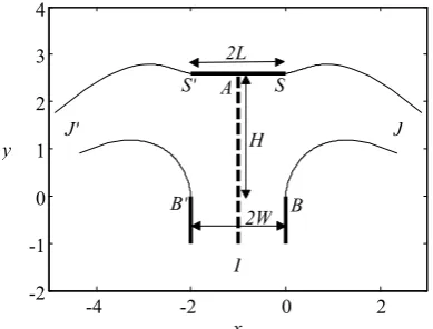
placed at a vertical distance H from the edges of the pipe and falling symmetrically under gravity. As shown in Fig. 1, the stream coming from far inside the pipe (see point I) hits the horizontal wall, centered at point A, and forms two jets – one on each side – detaching at points B (B) and S (S) and forming free surfaces BJ (BJ) and SJ (SJ) to the
Impact of Fluid Streams on Horizontal Walls
right (left).
Due to symmetry, the formulation of the problem is based on the ‘right’ half of the flow. The results presented in the sequel are simply obtained by superposition of the ‘left’ and ‘right’ flows. The coordinate system to be used is (x, y), x
being horizontal and y vertical. The point B is taken as the origin (see Fig. 1). The mass flux emerging from the ‘right’ pipe is
Q = UW. (2) Let u and v denote the x- and y-components of the fluid velocity. The system is assumed to be governed by irrotationality and incompressibility. This leads to (u, v) = , with Laplace’s equation 2 = 0 holding for the velocity
potential . Bernoulli’s equation then follows as a first integral of the Euler (momentum) equations of motion and reads
, constant )
( 2 2
2
1
p gy v
u (3)
which is valid everywhere inside the fluid and where p is the pressure and the fluid density. Assuming that the pressure has the same constant value p = 0 on all free surfaces, and taking W and U as the unit length and unit velocity respectively, Q becomes unity and Bernoulli’s equation on the free surfaces becomes, in dimensionless form,
. 1
)
( 2
2 1 2 2 2 2 1
B
v y F v
u (4)
[image:2.595.74.269.516.664.2]Here the same symbols are kept for the dimensionless variables for the sake of simplicity. The constant on the right-hand side has been evaluated at point B, where the velocity is purely vertical and y = 0.
Fig. 1. Sketch of the flow and of the coordinates. The free-surface profile is a computed solution for F = 2.0 and (xS, yS) = (0, 2.6). Special points are labeled on the boundary.
The problem under consideration can be solved with the use of conformal mappings. Hence, we introduce the complex variable z = x + iy, the complex potential f = +
(velocity potential (x, y), streamfunction (x, y)), and the hodograph variable
. )
( u iv
dz df
z
(5)
The domain of the fluid in the f-plane is then transformed into the upper half of the unit disk in a t-plane. The transformation from the f-plane to the t-plane can be written as
) 1 )( )( 1 (
1 )
1 ( 1
2 2 2
I I I
tt t t t
t t
dt df
. (6)
Note that the free surfaces in the t-plane are described by the points t = eiσ, σ[0, π].
The problem now reduces to finding the hodograph variable ζ as an analytic function of t, satisfying Bernoulli’s equation (4) on the free surfaces. Considering the singularities present, it turns out [16] that
, )]
1 ( ln [ ) (
)] 1 ( ln [ ) ( )
( 1/2 2 1/3 ( )
) ( 3 / 1 2 2
/ 1
I
t I A
I
t A
e t c t
t
e t c t
t i
t
(7)
where |ζ(tI)| = 1. The value of ζ does not depend on c. The
function Ω(t) here is analytic for |t|<1 and continuous for |t| 1, and can be expanded in a power series of the form
. )
( 1
n n nt
a
t (8)
III. NUMERICAL METHODS AND RESULTS
The coefficients an in the power series (8) can be
determined by using a collocation Galerkin method. We truncate the infinite series after N – 2 terms and introduce on the free surfaces the mesh points
), (
2 21
M
N
M
M = 1, … , N – 2. (9)
To compute the values of y in Bernoulli’s equation (4), use is made of the equation
, 1
dt df dt dz
(10)
which is integrated numerically. Substituting the expressions of y and ζ into equation (4) at the mesh points σM, we obtain N – 2 nonlinear algebraic equations for the N unknowns a1,
…, aN–2, tI and tA. The last two equations are obtained by
imposing the position of point S (xS, yS).
The solutions we consider form a three-parameter family of solutions. The three parameters are the Froude number F, the offset parameter xS (= L/W – 1), and the aperture
parameter yS (= H/W). When the offset is negative one
obtains underhanging configurations, while for positive offsets one obtains overhanging configurations. When xS = 0,
the edge of the wall is on the same vertical line as the side of the pipe. Of course, if the elevation of the wall is too high, the flow may not reach the wall, so there is an upper bound on yS.
-4 -2 0 2
-2 -1 0 1 2 3 4
x y
I J'
B B'
S S'
J A
2W 2L
In order to study systematically the three-parameter family of solutions, we let the offset of the wall and the aperture between wall and pipe vary for given values of the Froude number F. Imagine that the Froude number F is fixed and that one varies the size and the position of the wall. If the wall is short enough and not too high, then the flow will continue as two rising jets after hitting the wall. If the wall is long enough, the flow will follow the wall without rising any longer. It will eventually develop into two downward jets. If the wall is neither short nor long, the flow will look like a fountain (see Fig. 1).
We now present results, covering all cases, for F = 2.0. Note that the general behavior is the same for all Froude numbers.
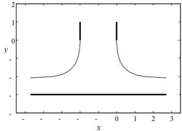
(a) ‘Rising’ jet. In this case, the stream is weakly diverted by the horizontal wall when hitting it, then continues to rise in the form of jets before eventually falling down under gravity. This is shown in Fig. 2 for (xS, yS) = (–0.4, 1.0).
(b) ‘Overhanging’ jet. In this case, the stream is strongly diverted by the horizontal wall when hitting it, then follows an almost horizontal trajectory in the form of jets before eventually falling down under gravity. This is shown in Fig. 3 for (xS, yS) = (1.3, 1.1). The solution shown here is
reminiscent of the limiting no-gravity case (F ∞, xS ∞).
(c) ‘Intermediate’ jet. In this case the stream rises slightly after hitting the wall, but then quickly falls down under gravity. An example was already shown in Fig. 1(a) for (xS, yS) = (0, 2.6). The flow looks like a fountain and the wall has
[image:3.595.315.528.389.509.2]only a small effect on the flow.
Fig. 2. Same as Fig. 1 for F = 2.0 and (xS, yS) = (–0.4, 1.0). We
refer to such flows as ‘rising’ jets.
Fig. 3. Same as Fig. 1 for F = 2.0 and (xS, yS) = (1.3, 1.1). We
refer to such flows as ‘overhanging’ jets.
IV. UPLIFT FORCE EXERTED ON THE HORIZONTAL WALL One of the most interesting features of the present application is the study of the lift FL exerted on the wall. It is
equal to the vertical component of the pressure force exerted
on the wall. Using Bernoulli’s equation (3), one obtains the following expression for the lift coefficient CL:
, ) (
) ( 1
1 ( )
1
2 2 2 )
(
1 2 2 1 2
2
1 U dx x S u u v dx
p L W L U F C
S x
S S
x L
L
(11) where uS is the velocity at point S. Since the flows depend on
three independent parameters it is not possible to perform a full parametric study. Fixing the Froude number we let the elevation of the wall yS vary for a discrete set of values of the
offset xS. The results are presented in Fig. 4. For some
parameters, the lift coefficient was found to be negative (see the middle and right plots). In other words, the wall is being sucked down by the flow rather than lifted up.
This somewhat counterintuitive result can be explained as follows. Along the wall SAS Bernoulli’s equation simply
reads 2.
2 1 2 2 1
S
u p
u At the centre of the wall (point A) the pressure is maximum since the velocity u is 0. At the edges of the wall (points
S
'
and S) the pressure is 0 (atmospheric pressure). In the limit as point S becomes a stagnation point (see §VI), the velocity uS becomes identically 0 and thereforethe pressure must be negative everywhere along the wall
( 2
2 1u
p ). On the middle and right plots, the upper bound for yS indeed corresponds to the formation of a stagnation
[image:3.595.73.265.410.536.2]point at the edge of the wall S.
Fig. 4. Lift exerted on the wall. Plot of the lift coefficient (11) as a function of the wall-elevation yS, for three different
values of the offset xS, for F = 2. Left: xS = –0.4; middle: xS =
0; right: xS = 1.3.
V. FALLING JETS
We now consider the ‘inverted’ case of a steady irrotational flow of an incompressible inviscid fluid falling from a pipe of width 2W under gravity, hitting a horizontal wall of infinite
length placed at a vertical distance H from the bottom edges of the pipe and splitting symmetrically into two jets one on each side of the pipe. As shown in Fig. 5, the stream coming from far inside the pipe (see points J, J) hits the horizontal wall, centered at point C, and forms two jets – one on each side – detaching at points A, A and forming free surfaces
AI, AI.
Following the formulation in §II, the corresponding transformation from the f-plane to the t-plane can be written as
) 1 (
1 1
t t
t dt
df
. (12)
- - - - 0 1 2
-0 1 2
x y
- - - 0 1 2 3
-0 1 2
[image:3.595.61.277.576.687.2]Fig. 5. Sketch of the flow and of the coordinates. The free-surface profile is a computed solution for H = 1.5 and F
= 1.5.Special points are labeled on the boundary. In this case, the hodograph variable is
, )
( ) ( )
( ()
2 / 1
2 / 1
t C
C e
t t t
t
(13)
where ζ(0) = i and Ω(t) is given as in (8). The parametrization
t = eiσ, σ[0, π], of the free surface in the t-plane and differentiation of Bernoulli’s equation (4) with respect to σ
yields
. 0 )
sin cos ( 1
2 2 2 1 2 1
2
v u
u F
vv uu
(14)
Substituting the expression of ζ into equation (14), at N mesh points σM we obtain N nonlinear algebraic equations for the N
unknowns a1, …, aN. Given F and H, this system is solved by
Newton’s method, giving a two-parameter family of solutions.
In Fig. 5, we have already shown a computed solution where the distance of the horizontal wall from the end of the pipe is H = 1.5 for a relatively large value of the Froude number F = 1.5. One can see that the flow leaves the pipe at A
(A) tangentially at an angle of 180o and gradually moves to
the right (left) forming a single-free-surface jet that moves along the horizontal wall to + (–). Keeping F fixed at 1.5 and letting H vary has the following effect in the behavior of flow. As shown in Fig. 6 for ‘small’ H = 0.2 the flow, after detaching, moves to the right (left) almost immediately and continues along the horizontal wall to + (–). For ‘large’ H
= 3.0 (see Fig. 7) the jet becomes thinner (i.e. the fluid is like being squeezed) after detaching, then is gradually diverted and finally moves along the horizontal wall to + (–).
[image:4.595.58.272.58.186.2]Fig. 6. Same as Fig. 5 for H = 0.2 and F = 1.5.
Fig. 7. Same as Fig. 5 for H = 3.0 and F = 1.5 (N = 400). Increasing the Froude number to ‘large’ values has no effect on the behavior of the flow for small to medium heights H. This behavior though, persists even for large values of H, as demonstrated in Fig. 8, where F = 10 and H = 3.0. One can observe that there is no squeezing of the free surfaces. In fact, for H = 3.0, the transition value of F
(separating the regions with and without squeezing) is 3.3. On the other hand, decreasing the Froude number to relatively low magnitude has the effect that the squeezing of the free surfaces occurs regardless of the magnitude of the height H. For instance, n fact, for H = 1.5, the transition value of F (separating the regions with and without squeezing) is 0.93.
Fig. 8. Same as Fig. 5 for H = 3.0 and F = 10.
The curve along which the transition between squeezing and no-squeezing occurs is shown in Fig. 12 (see §VI). It is the curve that separates region I from region II.
VI. FLOWS WITH A STAGNATION POINT
A. RISING FLOWS
For the case of rising flows, if one wishes to impose the condition that the edges of the horizontal wall S and
S
'
are stagnation points, then – following the formulation in §II – the hodograph variable is
, )] 1 ( ln [ ) ( ) 1 (
)] 1 ( ln [ ) ( ) 1 ( )
( 2/3 1/2 2 1/3 ( )
) ( 3 / 1 2 2
/ 1 3 / 2
I
t I A
I I
t A
e t c t
t t
e t c t
t t i
t
[image:4.595.331.518.391.526.2] [image:4.595.59.269.644.775.2] (15)
where |ζ(tI)| = 1 and Ω(t) is given as in (8). Substituting the
expressions of y and ζ into equation (4), at N – 2 mesh points
-5 -4 -3 -2 -1 0 1 2 3 -2.5
-2 -1.5 -1 -0.5 0 0.5 1 1.5 2
x y
J J
H 2W
I I
A A
C
-3 -2 -1 0 1
-3 -2 -1 0 1
x y
-2.5 -2 -1.5 -1 -0.5 0 0.5 -0.4
-0.2 0 0.2 0.4 0.6 0.8 1 1.2
x y
- - - 0 1 2 3
-0 1 2
σM we obtain N – 2 nonlinear algebraic equations for the N
unknowns a1, …, aN–3, F, tI and tA. The last two equations are
obtained by imposing the position of S. Again, this system of
N nonlinear equations in N unknowns is solved by Newton’s method.
We first study the effect of the position of the stagnation point S on the Froude number F. For three ‘extreme’ values of xS, namely –0.95, 0 (the wall length and the pipe width are
[image:5.595.331.514.116.242.2]equal) and 1, i.e. letting the horizontal wall vary from very short to long, the resulting relation F vs yS is demonstrated in
Table 1. It turns out that the x-coordinate of the stagnation point has very little effect on the relation F vs yS. Of interest is
the fact that when xS = 1 (long wall), there is a limiting wall
elevation at about yS = 0.42. If the wall is lowered below that
value, the flow will not be able to reach the end of the wall and will detach before the edge of the wall. This limiting behavior occurs for all positive values of xS.
Table 1. Values of the Froude number F as a function of xS
and yS for flows with a stagnation point. xS
yS
–0.95 0 1 0.1 0.019 0.018 - 0.2 0.053 0.052 - 0.42 0.159 0.155 0.205
0.6 0.267 0.261 0.338 1.0 0.547 0.538 0.636 1.4 0.852 0.841 0.923 1.8 1.155 1.145 1.201 2.0 1.302 1.293 1.337 2.4 1.583 1.577 1.600 2.8 1.844 1.840 1.849 3.0 1.966 1.963 1.959
Fig. 9 shows the computed solution for a long horizontal wall with (xS, yS) = (1.0, 3.0), yielding F = 1.96. Finally Fig.
10 shows the computed solution for a very short horizontal wall with (xS, yS) = (–0.99, 1.64), yielding F = 1.04. This can
be compared with the limiting case of no horizontal wall. In fact solutions of this kind (in the absence of horizontal wall) were computed in [5].
Fig. 9. Free-surface profiles with stagnation point at (xS, yS) =
(1.0, 3.0). The Froude number F = 1.96 comes as part of the solution.
Solutions have been found to exist only for values of F
greater than a certain critical value F0. For example, with
(xS, yS) = (–0.68, 1.20), the critical value F0 is roughly 0.70.
[image:5.595.66.218.295.456.2]The free-surface profiles are shown in Fig. 11 and are reminiscent of the weir flows [18]–[19]. The effect of the stagnation point is so local that it barely influences the whole flow.
Fig. 10. Same as Fig. 9 for (xS, yS) = (–0.99, 1.64). The
[image:5.595.324.523.334.490.2]Froude number F = 1.04 comes as part of the solution. The wall is so small (total length of 0.02) that it cannot be seen on the figure. Points A (centre of the wall) and S (edge of the wall) are both stagnation points but they have different singular behavior.
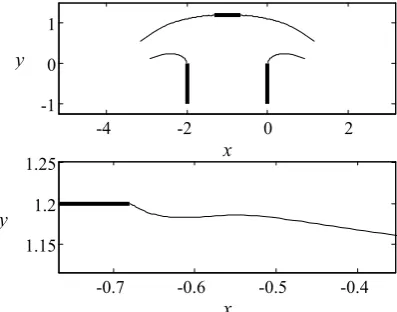
Fig. 11. Same as Fig. 9 for (xS, yS) = (–0.68, 1.20) and F =
0.70, and the blow-up of the upper right free surface near the stagnation point S.
B. FALLING FLOWS
For the case of falling flows, if one wishes to impose the condition that the flow exhibits stagnation points at the ends of the pipe A and
A
'
, As in the simplified configuration of a falling jet in the absence of the horizontal wall [10], the only possible values for the angles between the vertical side of the pipe and the free surface are 90o and 120o. The 90o casecorresponds to the free surface leaving the side of the pipe horizontally, while the 120o case corresponds to the free
surface leaving the side of the pipe at a 60o angle from the
vertical. Following the formulation in §II, the hodograph variable is
) ( 2
/ 1
2 / 1 3 / 2
) (
) ( ) 1 ( )
( t
C
C e
t t t t
t
or ,
) (
) )( 1 ( )
( ()
2 / 1
2 / 1
t C
C e
t t t t
t
(16) where ζ(0) = i and Ω(t) is given as in (8) Substituting the expressions of ζ into equation (14), at N mesh points σM we
- - - 0 2 4
-0 1 2 3 4
x y
- - - - 0 1 2
-0 1 2
x y
-4 -2 0 2
-1 0 1
x y
-0.7 -0.6 -0.5 -0.4
1.15 1.2 1.25
[image:5.595.63.268.567.694.2]obtain N nonlinear algebraic equations for the respectively N
unknowns a1, …, aN–1, F, giving a one-parameter (for H)
family of solutions (120o-case), or a
1, …, aN, giving a
two-parameter (for F and H) family of solutions (90o-case).
[image:6.595.58.273.140.264.2]Once more, these systems of equations are solved by Newton’s method.
Fig. 12. The two plotted curves divide the (F, H/W) plane into three regions. In region I, the jet emerges from the pipe without a stagnation point and is immediately deflected. In region II, the jet emerges from the pipe without a stagnation point but experiences squeezing before being deflected by the horizontal wall. In region III, the jet emerges from the pipe with a stagnation point.
It turns out that flows exhibiting a stagnation point of 120o
exist only for ‘small’ Froude numbers, Fs 0.50 = Fcr.
Actually, this critical value Fcr corresponds exactly to the one
found in [10] (note that by definition the Froude number of the present paper is equal to 2 times the Froude number in that paper). The curve that gives Fs as a function of the
elevation H is given in Fig. 12. It is the boundary between regions II and III. As H increases, Fs approaches the limiting
value of 0.5, which corresponds to the configuration in the absence of the horizontal wall. A typical flow is shown in Fig. 13 for H = 1.01, corresponding to a Froude number of F
= 0.35. One can see that the flow detaches at A (A) at an angle of 120o and gradually turns to the right (left) and moves
[image:6.595.356.497.163.285.2]along the horizontal wall to + (–). Note that the same results can be obtained through the formulation in §V but the convergence is not as good. The reason is that the singularity is so local that it does not affect much the rest of the solution.
Fig. 13. Free-surface profiles with 120o stagnation points at
A, A for H = 1.01. The Froude number F = 0.35 comes as part of the solution.
On the other hand, flows exhibiting a stagnation point of 90o exist for ‘small’ Froude numbers (F < F
cr, see the 120o
case) for values of H larger than the value of H corresponding to the 120o case. For instance, for F = 0.35 such solutions
exist for 1.01 H, where 1.01 is the corresponding H for the 120o case. An example of a flow with 90o stagnation points is
demonstrated in Fig. 14 for H = 0.5 and F = 0.1. Such solutions fall into region III of Fig. 12 above.
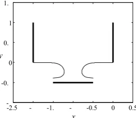
Fig. 14. Free-surface profiles with 90o stagnation points at A,
A for H = 0.5 and F = 0.1 (N = 400).
REFERENCES
[1] J.-M. Vanden-Broeck, and J.B. Keller, “Jets rising and falling under gravity,” J. Fluid Mech. 124, pp. 335–345, 1982.
[2] C. Clanet, “On large-amplitude pulsating fountains,” J. Fluid Mech.
366, pp. 333–350, 1996.
[3] F. Dias, and J.-M. Vanden-Broeck, “Nonlinear bow flows with spray,”
J. Fluid Mech. 255, pp. 91–102, 1993.
[4] F. Dias, and J.-M. Vanden-Broeck, “Flows emerging from a nozzle and falling under gravity,” J. Fluid Mech. 213, pp. 465–477, 1990. [5] F. Dias, and P. Christodoulides, “Ideal jets falling under gravity,” Phys.
Fluids A 3(7), 1711–1717, 1991
[6] J. Lee, and J.-M. Vanden-Broeck, “Two-dimensional jets falling from funnels and nozzles,” Phys. Fluids A 5, 2454–2460, 1993.
[7] J. Lee, and J.-M. Vanden-Broeck, “Bubbles rising in an inclined two-dimensional tube and jets falling along a wall,” J. Austral. Math.
Soc. Ser. B 39, 332–349, 1998.
[8] P.R. Garabedian, “On steady-state bubbles generated by Taylor instability,” Proc. R. Soc. Lond A 241, 423–431, 1957
[9] G. Birkhoff, and D. Carter, “Rising plane bubbles,” J. Mathematics and
Mechanics 6 (4), 769–779, 1957.
[10] J.-M. Vanden-Broeck. “Bubbles rising in a tube and jets falling from a nozzle,” Phys. Fluids 27 (5), 1090–1093, 1984.
[11] B. Couet, and G.S. Strumolo, “The effects of surface tension and tube inclination on a two-dimensional rising bubble,” J. Fluid Mech. 184, 1–14, 1987.
[12] N.A. Inogamov, and A.M. Oparin, “Bubble motion in inclined pipes,”
JETP 97, 1168–1185, 2003.
[13] T.B. Benjamin, “Gravity currents and related phenomena,” J. Fluid
Mech. 31, 209–248, 1968.
[14] E.O. Tuck, and A. Dixon, “Surf-skimmer planing hydrodynamics,” J.
Fluid Mech. 205, 581–592, 1989.
[15] H. Michallet, C. Mathis, P. Maissa, and F. Dias, “Flow filling a curved pipe,” Transactions of the ASME J. Fluids Engineering 123, 686–691, 2001.
[16] P. Christodoulides, and F. Dias, “Impact of a rising stream on a horizontal plate of finite extent,” J. Fluid Mech. 621, 243–258, 2009. [17] P. Christodoulides, and F. Dias, “Impact of a falling jet,” J. Fluid
Mech., in print.
[18] J.-M. Vanden-Broeck, and J.B. Keller, “Weir flows,” J. Fluid Mech.
176, 283–293, 1987.
[19] F. Dias, J. Keller, and J.-M. Vanden-Broeck, “Flows over rectangular weirs,” Phys. Fluids 31, 2071–2076, 1988.
0 0.5 1 1. 2 2.5
0 0.
1 1.
2 2.
3
H/W
I
III I
-2.5 - -1. - -0.5 0 0.5
--0. 0 0.
1 1.
x y
- -2. - -1. - -0.5 0 0. 1 -1.
--0. 0 0.5 1 1.5
x y
[image:6.595.75.259.590.720.2]