Modeling and Analysis of the Dynamics of Load Carrying System



Abstract—In this work, the problem of modeling and analyzing of dynamic effects of crane’s load carrying system has been considered. The initial problem of the motion of load carried by the forest crane during the working cycle has been formulated and solved. Friction effects are taken into consideration. The workout calculation model enables one to analyze the motion of the load under influence of kinematical forcing and the free vibration of the load as the result of the previous forced motion. The exemplary results of the numerical simulation are presented.

Index Terms— analysis, crane, dynamics, friction, modeling,

multibody system.

I. INTRODUCTION

The problems of modeling and analysis of dynamical phenomenon of heavy construction machines and their components have been a subject of many works. In paper [1], B. Posiadala et al. have presented the formulation and solution of initial value problem representing the motion of load carried by a truck crane. The load is considered as a particle. The motion of the load under influence of kinematic forcings and its further free motion have been investigated. In works [2], [3], B. Posiadala has developed the model of the system by including the influence of flexibility of the rope and crane supporting system. The model of dynamics of the system, representing the main machine elements, including the support system, coupled with the load has been obtained. In paper [4], A. Maczynski has presented the model and the investigation results concerning the minimizing of load oscillations in rotary cranes.

In works [5], [6], B. Posiadala at al. have presented the formulation and solution of initial value problem representing the motion of the load carrying system considered as the systems of rigid bodies. In this work, this model has been developed by including friction effects in revolute joints of the system. The formulation and solution of the initial problem, based on the developed model, as well as the exemplary results of numerical simulations are

Manuscript received July 9, 2012; revised July 28, 2012.

The study was carried out within statutory research BS/PB-1-101-3020/11/P of the Institute of Mechanics and Machine Design Foundations of the Czestochowa University of Technology.

B. Posiadala is with the Institute of Mechanics and Machine Design Foundations, Czestochowa University of Technology, Czestochowa, Poland (e-mail: bogdan.p@imipkm.pcz.pl).

M. Tomala is with the Institute of Mechanics and Machine Design Foundations, Czestochowa University of Technology, Czestochowa,

presented.

II. COMPUTATIONAL MODEL

In this work, the load carrying system of a forest crane has been investigated and its kinematical configuration has been taken into account. The computational model is shown on Fig. 1. The system consists of three rigid bodies connected with each other by revolute joints P and Q. The body I is connected with the end of the boom by the revolute joint Ω.

The Cartesian coordinate system OXYZ and four generalized coordinates: φ, θ1, θ2 and Φ have been introduced to develop the mathematical model. The motion of each body of the system can be described using these coordinates and their time derivatives. The φ coordinate is one of control parameters of the crane. This coordinate describes a position of lifting plane and is closely related to

rΩ vector components. The problem of formulating components of this vector in global frame as functions of time has been presented in works [1]-[2]. In these works, typical groups of cranes and typical working cycles have been taken into consideration. The Φ coordinate describes the rotation angle of gripper and load and also is a control parameter. A correct formulation of φ, Φ and rΩ functions opens the way to model any working cycle of the crane. Angular coordinates θ1 and θ2 describe a dynamic response of the system and they are obtained as the solution of initial value problem.

Additionally, three local frames have been introduced into the model and their origins are placed in the revolute joints of the system. Every frame is oriented in such way that one of its axes is a pivot. For the Ω joint the axis of rotation is

Modeling and Analysis of the Dynamics

of Load Carrying System

Bogdan Posiadala, Mateusz Tomala

yΩ, for P joint – xP axis. This way of defining of the local

frames simplifies the consideration of the friction effects in each revolute joint.

III. FORMULATION AND SOLUTION OF INITIAL VALUE PROBLEM

The equations of the system motion have been obtained using Lagrange equations of the second kind. The system has two angular degrees of freedom: θ1 and θ2. Lagrange equations of the second kind for the considered system can be written as:

2 , 1 , θ

θ   

            k M L L dt d k k k

 , (1)

where L is the Lagrangian and Mk (k = 1, 2) are

computational moments which act about Ω and P points, respectively. The Lagrangian is defined as a total kinetic energy of the system minus its total potential energy:







K E E E

E

L . (2)

The equations of motion of the system consist the system of ordinary differential equations (ODE). Computational moments of forces Mk depend only on the instantaneous

configuration of the system and on friction law which is taken into account. In this work, simple Coulomb friction law is considered and according to this the force of friction is a linear function of the radial force in the joint:

) ( ) ( μ k k N

T  , (3)

where μ is a generalized friction coefficient. Additionally, different coefficients of static and kinetic friction are taken into consideration. According to the Karnopp assumption [7], the interval of small velocities <-ε,ε> is considered. In this interval it is assumed that the velocity is equal to zero and static friction coefficient is taken into account. The simplified formula describing the friction coefficient versus

generalized velocity is shown in the Fig. 2.

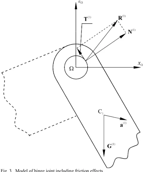
In the considered model the clearance or deformation effects have been neglected, thus the motion parameters depend only on generalized coordinates (φ, Φ, θ1 and θ2) and their time derivatives. Components of reaction forces (Fig. 3) could be obtained using Newton equations:

3 , 2 , 1 , ) ( ) (   i

m_iai Si , (4)

where miis i-th body’s mass, a(i) is the absolute acceleration

of center of mass of the body and S(i) is the total force acting on it.

Total forces can be written as following sums:

, , , ) 3 ( ) 3 ( ) 3 ( ) 2 ( ) 2 ( ) 3 ( ) 2 ( ) 1 ( ) 2 ( ) 1 ( ) 1 ( G R S G R R S G R R S          (5)

where G(i) is i-th body’s gravity force. If reaction forces R(i)

and their components in a global frame are known, each reaction force component (radial or axial) can be easily defined. For i-th joint, a resultant reaction in rotation plane is a sum of tangent and radial reaction forces:

) ( ) ( )

(k k k

N T

R   . (6)

Equation (6) is a vector equation and can be rewritten into the scalar form using proper components. If one projects this equation onto the proper rotation plane (ΩxΩzΩ for the Ω joint and PyPzP for the P joint), it is equivalent to two scalar

equations. Next step is to rewrite (3) into the scalar form: 2 2 2 1 2 2 2

1 T μ N N

T    . (7) Fig. 2. The friction coefficient versus generalized velocity.

It is necessary to take into account that the T and N

vectors are always perpendicular, so their scalar product is always equal to zero. This condition, (3) and (6) previously rewritten into the scalar form are together a system of four equations. Each reaction force component (radial and tangent) can be computed from the equation system:

            0 μ ) ( ) ( ) ( ) ( ) ( ) ( ) ( k k k k k k k N T N T R N T

. (8)

Moment of friction force (static or kinetic) acting on cylindrical surfaces of journal and bearing can be obtained using absolute value of friction force:

) ( ) 1 ( 2 k k T k d

M  T , (9)

where dkis a diameter of k-th hinge joint.

In this work, moments of friction forces acting on side (retaining) surfaces are taken into account, as shown on Fig. 4.

If one considers that the side surface has a shape of ring, the moment of friction force can be obtained using a following formula: 2 1 2 1 2 1 2 1 ) ( ) 2 ( μ 3 2 r r r r r r

M T k

k

  

 F , (10)

where F(k) is an axial force in k-th joint, r1 and r2 are internal

and external radii of the ring, respectively. F(k) force acts along proper direction for each joint. For Ω joint F(k) force acts along yΩ axis, for P joint - along xP axis. One can notice

that at every step of time in each joint only one of two retaining surfaces is under pressure. It means that the moment of side friction acts only on one side of each joint.

Total moments of friction forces are sums:





 

) 2 ( ) 1 ( )

( T _sgnθ

k T k T

k M M

M   . (11)

Values of computational moments can be obtained with following scheme:                   ε θ ε θ ε θ ) ( ) ( ) ( ) ( ) ( ) ( ) ( k T k G k k T k G k k T k T k G k

k M M

M M for M M M M    , (12)

where Mk(G) is k-th moment of conservative forces acts in k

-th joint.

IV. EXEMPLARY RESULTS OF NUMERICAL COMPUTATION The exemplary results of numerical calculations have been obtained for the system parameters shown in Tables I, II and III.

Fig. 4. Friction effects on a retaining ring.

TABLEI

EXEMPLARY COMPUTATION –PROPERTIES OF BODIES

Parameter Value(s)

Body I Body II Body III Dimensions

x×y×z [m] 0.1×0.15×1 0.15×0.1×0.9 3×0.4×0.6

Density

ρ [kg·m-3_] 7700 7700 900

Mass

m [kg] 115.5 103.95 648

TABLEII

EXEMPLARY COMPUTATION –PROPERTIES OF JOINTS

Parameter Value(s)

Ω P

Static friction

coefficient µS [-] 0.2 0.3 Kinetic friction

coefficient µK [-] 0.1 0.2 Radius of journal

(internal radius of retaining ring) [m]

0.05 0.04

External radius of

retaining ring [m] 0.06 0.05 Interval of static

friction [rad·s-1_] 10-6 10-6

TABLEIII

EXEMPLARY COMPUTATION –INITIAL POSITION OF THE CRANE

Parameter Value(s)

XΩ [m] 2.898

YΩ [m] 0

ZΩ [m] 5.298

Initial value of φ [rad] 0

The considered system consists of three rigid bodies with dimensions and mass parameters as given in Table I. First two bodies are made of steel, the third (a load) is made of wood. The presented results of calculations include the initial equilibrium state, the motion of the load carrying system according to the working cycle represented by so-called kinematic forcings and further free motion as the result of previously forced motion.

A working cycle which has been chosen for the exemplary computation is characterized by the changes of time derivatives of generalized coordinates φ and Φ versus time as shown in Fig. 5. The chosen kinematical forcings include the rotation of crane boom starting in 3rd second and the rotation of the gripper with load starting in 7th second. Properties of joints (friction coefficients, dimensions of joints, etc.) are listed in Table II. In Table III, the initial position of Ω point (end of the crane boom) in global frame and initial values of angles φ and Φ are presented.

The solution of the initial value problem is obtained numerically, using the Runge-Kutta method of the fourth-order and the performed computational program. In the program the variable integration step has been used and its maximum value was equal to 0.001 second.

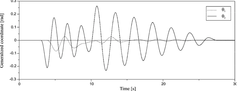
The solution results of the initial value problem are represented by the generalized coordinates (Fig. 6) versus time. For the considered case the trajectory of the crane boom end (the Ω point) and trajectories of centers of masses of each body in the global frame have been determined. The

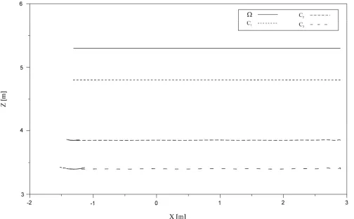
OXY trajectory projection is shown on Fig. 7 and the OXZ

projection is shown on Fig. 8.

The total energy of the system has also been computed and its changes versus time for the considered case are shown in Fig. 9. The computation of the total energy of the system using the motion parameters, obtained as the initial problem solution, enables one to follow the changes of this value. This is helpful to recognize the correctness of the obtained numerical results.

V. CONCLUSION

In this work, the problems of modeling and analyzing of dynamic effects of crane’s load carrying system have been considered. The formulation and solution of the initial value problem of dynamics of load carrying system have been presented. Friction effects have been taken into consideration with different static and kinetic friction coefficients.

Fig. 5. The exemplary computation – kinematical forcings used in the simulation.

The worked out computational model enables one to analyze the dynamical behavior of the system of the chosen configuration during the machine working cycle. The solution is valid for the forced motion, according to the kinematic forcings, and for further free motion of the

system, according to the initial conditions resulting from the previous motion.

The proposed model could be used to study the dynamics of other multibody systems equipped with revolute joints including the friction effects. The mathematical model could Fig. 7. The OXY projection of trajectories: of the mass centers C1, C2, C3 and of the boom end Ω.

be extended by introducing joint clearances and deformation. The model could also be extended by introducing external influences.

REFERENCES

[1] B. Posiadala, B. Skalmierski, L. Tomski, “Motion of Lifted Load Brought by Kinematic Forcing of the Crane Telescopic Boom”, Mechanism and Machine Theory, Vol.25, No. 5, 1990, pp.547-556. [2] B. Posiadala, “Influence of crane support system on motion of the

lifted load”, Mechanism and Machine Theory, Vol. 32, No. 1, 1997, pp.9-20,

[3] B. Posiadala, Modeling and analysis of dynamical phenomenon of heavy construction machines and its elements as discrete-continuous mechanical system, Publishing House of Czestochowa University of Technology, series Monographs no 61, 1999 (in Polish),

[4] A. Maczynski, “Load positioning and minimization of load oscillations in rotary cranes”, Journal of Theoretical and Applied Mechanics, 41(4), 2003, pp.873-885,

[5] B. Posiadala, M. Tomala, “Computational model of the motion of the load carried by the binomial grab system”, Modelowanie inżynierskie (Engineering Modeling), Vol. 10, No. 41, 2011, pp.323-330 (in Polish),

[6] B. Posiadala, M. Tomala, P. Warys, “Modeling and analysis of dynamics of crane load carrying system”, Mechanik (Mechanic), 12, 2011 (electronic in Polish),

[7] D. Karnopp, “Computer simulation of stick-slip friction in mechanical dynamic systems”, Journal of Dynamic Systems, Measurement and Control, Vol. 107, 1985.