Stability and robustness of adaptive pole zero placement algorithm

STABILITY AND ROBUSTNESS OF ADAPTIVE POLE-ZERO PLACEMENT ALGORlTHM

A thesis

presented for the degree of

Doctor of Philosophy in Electrical Engineering in the

Uni versity of Canterbury Chri stchur ch. New Zealand

by

Chan Chok You

'I b 1987····

~Q/~~

~

LA,

Q;~,

aruL

~

b~~

~~~.

&~3:1

i

ABSTRACT

A computationally efficient pole-zero placement algorithm for e icit adaptive control of discrete-time plants is presented, It j.s effecti vely an impl ici t algori thm in the sense that the controller design stage is trivial. Although the algorithm is restricted to open-loop stable plants, it is applicable to nonminimum phase plants.

Resul ts concerning the adapti ve control of linear, time-invari ant plants having purely deterministi c or stochasti c disturbances are ven. In the deterministic case, it is shown that the adaptive control algorithm ensures that the purely deterministic disturbances ar e removed from the system out put and that asymptotic perfect tracking is achieved. In the stochastic case, it is shown that the adaptive control algorithm leads to the required stability properties of the closed-loop system.

ACKNOWLEGEMENTS

I would like to thank my supervisor, Dr. H.R. Sirisena, for his guidance and advice during the course of my study.

I would also like to thank Dr. L. Praly of CAl -Ecole des Mines de Paris for his helpful discussions.

i i i CONTENTS ABSTRACT ACKNOWLEDGEMENTS i i i CHAPTER CHAPTER 2

CHAPTER 3

INTRODUCTION

POLE-ZERO PLACEMENT 2.1 Introduction

2.2 Review of Existing Pole-zero Placement Approaches

9 9

2.2.1 Pole placement 10

2.2.2 Pole-zero placement (Astrom and Wi

tten-mark 1980) 12

2.2.3 Pole-zero placement (Lin and Chen 1986) 14 2.3 Development of Pole-zero Placement 17 2.3.1 Special case: All process poles cancelled 19 2.3.2 Special case: No process zeros cancelled 20 2.4 Choices of Pole-zero Polynomials 21

2.4.1 Deadbeat controll ers 21

2.4.2 Nondeadbeat response 22

2.5 Review of Multivariable Pole Placement (Prager

and Wellstead 1981) 23

2.6 Development of Multivariable Pole-zero Placement

Algorithm 24

2.6.1 Special case: All process poles cancelled 26 2.6.2 Special case: No process zeros cancelled 26

2.7 Alternati ve Formulation 27

2.8 Conclusion 28

ADAPTIVE CONTROL OF DETERMIN ISTIC SYSTEMS 3.1 Introduction

3.2 Pole-zero Placement Strategy for Known Plants 3.2.1 Deterministic disturbances

3.2.2 Pole-zero placement 3.3 Parameter Estimation Algorithms

3.3.1 Least squares

3.3.2 Constrained least squares 3.4 Pole-zero Placement Adaptive Control

3.5

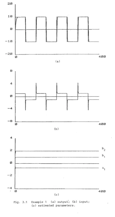
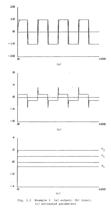
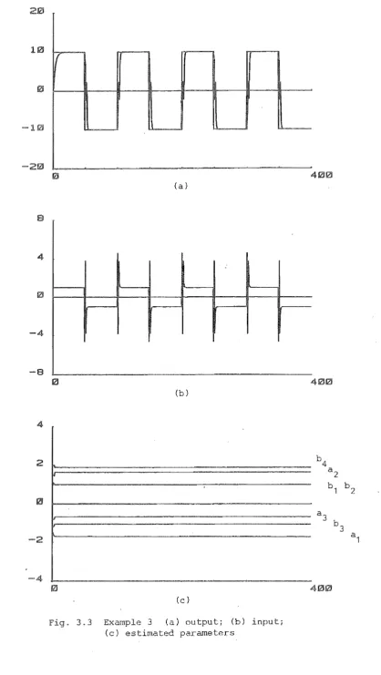
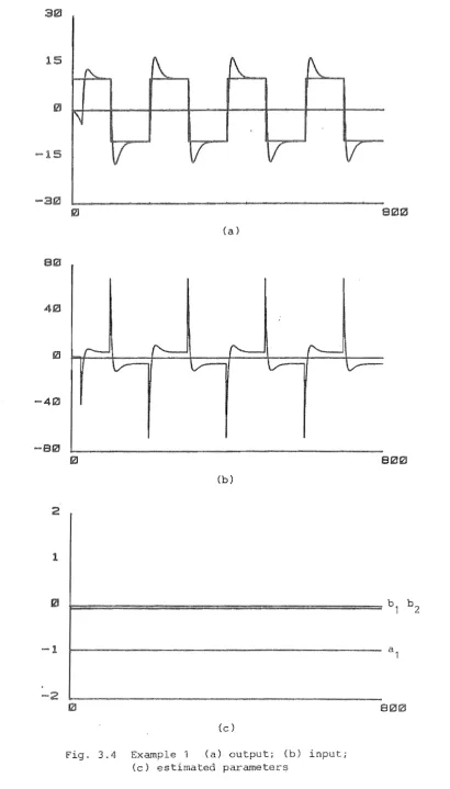
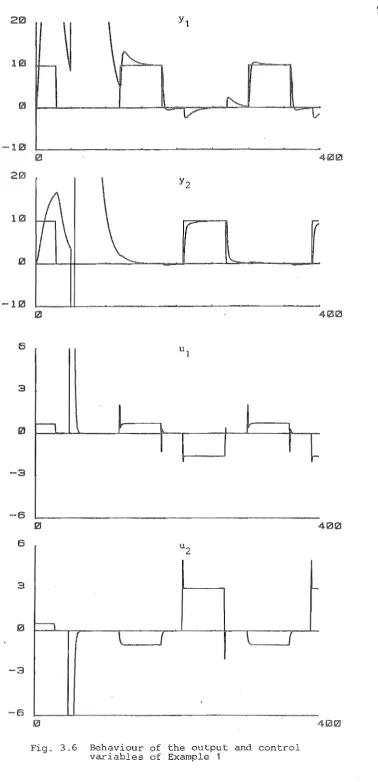
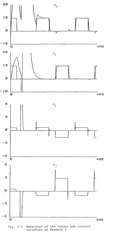
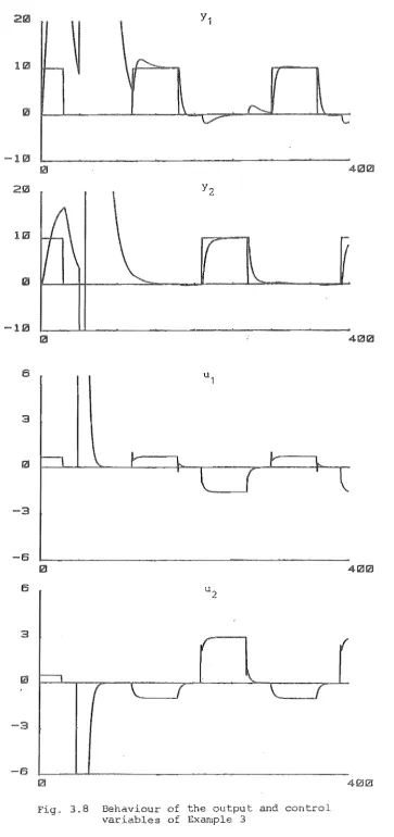
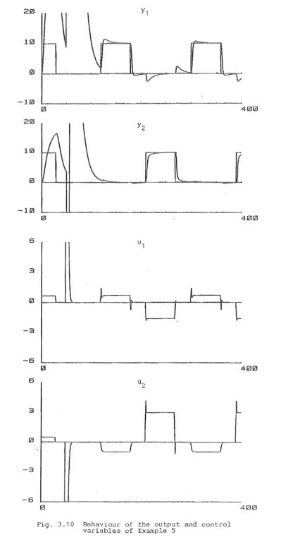
3.6 Robustness: Examples

CHAPTER 4

CHAPTER 5

3.7 Multi-input Multi-output Systems 3.7.1 Problem statement

3.7.2 The adaptation algorithm

3.8 Exampl es 3. 9 Concl usi on

ADAPTIVE CONTROL OF STOCHASTIC SYSTEMS

~.1 Introduction

4.2 Pole-zero Placement Str y for Knovm Plants

53 53 54 56 63 64 64 64

~.2.1 Deterministic and stochastic disturbances 65

~.2.2 Pole-zero placement

~.3 Adaptive Control: White Noise Case 4.3.1 Problem statement

4.3.2 The adaptation algorithm 4.3.3 Stability analysis

4.3.4 Convergence analysis

4.4 Adaptive Control: Coloured-Noise Case 4.4.1 Problem statement

4.4.2 The adaptation algorithm 4.4.3 Stability analysis

4.4.4 Convergence analysis

4.5 Conclusion

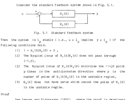
ROBUSTNESS: FIXED STRATEGY

5.1 Introduction 5.2 Preliminaries

5.3 Classi cal Stabil ity Theorems

5.4 System Structure

5.4.1 Higher-order systems 5.4.2 Nonlinearities

5.5 Robustness of Fixed Strategy

5.5.1 Output error 5.5.2 Input error

5.6 Instability of Fixed Strategy

5.7 Robust Disturbance Attenuation

5.8 Examples

5.9 Concluding Remarks

CHAPTER 6

CHAPTER 7

REFERENCES APPENDIX

ROBUSTNESS: ADAPTIVE CASE 6.1 Introduction

6.2 The Plant and Control Objective 6.3 The Adaptation Al gorithm

6.3.1 The control calculation

6.3.2 Parameter estimation algorithm 6.4 Properties of the Adaptive Controller 6.5 Conditions for Stability

6.6 Conclusion

CONCLUSIONS

7.1 Adapti ve Controller Based on Pole-zero Placement 7.2 Further Areas of Study

THE DECOUPLING PROBLEM

v

11 3

113 113 116 116 117 124

1

134

135 135 136

INT RODUCT ION

The idea of adapti ve control had its ori gi n in the earl y 1950' s. However, due to lack of theory and implementation difficul ti es interest waned. I t was not until the early 1970's that these stumbling blocks were overcome and interest was renewed. An excellent survey of the adapti ve control field is provided by Astrom (1983).

But what is adaptive control? It is not easy to define. In fact, a good defintion seems hard to come by in spite of the vast literature that exists on adaptive control. Astrom (1983) takes the view that i t is a special type of nonlinear feedback control. For Goodwin and Sin (1984), it is a type of control problem when the plant models and disturbances are not completely specified. However, the concepts involved are simple. An adapti ve controller generally consists of two elements one that identifies the plant parameters and the other which adj usts the controller parameters.

The two different approaches to adaptive control that have attracted much interest are model reference adapti ve control and self-tuning control.

The basic idea in model reference adaptive control is to cause the system to behave like a given model. Landau (1979) gi ves a comprehensive study of work up to 1977.

The idea of self-tuning control seems due to Kalman (1958). It was later revived by Astrom and Wittenmark (1973) who developed the self-tuning regulator in a stochastic framework and showed that the algorithm has some nice properties based on the convergence of the estimated parameters. Subsequently, Clark and Gawthrop (1975) provided some modifications to the ori ginal self-tuning regulator. Since then, numerous papers on the subject have appeared.

2

Host of the earlier works on adapti ve control have concentrated on al gori thmi c implementation and simulation of linear systems. Later.

proofs of convergence for the different versions of the adapt controller appeared. By convergence, it is meant that the control objecti ve is asymptotically achieved and all input and output si s remain bounded for any bounded initial conditions. Various assumptions on the plant are required to develop a convergent adapti ve control scheme.

There are several surveys on the convergence theory of adapti ve control algorithms ( e.g., Goodwin et al 198~. Kumar 1985 ). The latter provides a comprehensive survey of results on stochastic adaptive control.

Complete stability and convergence results have now been obtained for minimum phase deterministic and stochastic systems ( see the surveys by Goodwi n et al 198~ and Kumar 1985 ). The res ul ts are restricted to the model reference type control algorithms, wh.ich used pole-zero cancellation methods.

Model reference adaptive control algorithms have been developed ei ther in a continuous-time or in a discrete-time framework. I t would appear that the continuous-time algori thms can be implemented di tally w.i th li ttle error i f the sampling per.iod is suff.iciently small. However. Astrom et al (1984) have demonstrated that all continuous-time systems with poles excess larger than two wUl always give sampled systems with unstable zeros. This leads to the conclusion (M'saad et al 1985) that nonminimum phase characteristic are much more prevalent for sampled data systems than for continuous-time ems. A consequence of this is that discrete-time model reference control is ruled out. On the other hand, there are many results pertaining to continuous-time model reference control of such s

However, the problem of the adaptive control of nonminimum phase systems based on more complicated design procedures has not been completely solved. The principal difficulty with the proposed approaches has been that a stabilizabUity or controllability condition over the estimated model may arise. A comprehensive review of the problem of designing adaptive controllers for nonrninimurn phase systems is given by M'saad et al (1985).

Despite this difficulty, a number of stability results have been obtained. For example, in Elliot, Cristi and Das (1985),

Anderson and Johnstone (1985), Goodw.tn and Teoh (1985) global stability has been established on the basis of persistency of excitation, or parameter convergence. Thi s requirement may be removed by introducing a correction procedure to the parameter estimates (e.g., De Larminat

198~, Lozano and Goodwin 1985). In Kreisselmeier (1985), a continuous

~ ti me adapti ve control approach is made whi ch requires the pl ant parameters to lie in a knmm convex set where no unstable pol e- zer 0

cancellation occurs.

It should be stressed that the preceding stability results have been establ.i.shed only for deterministic nonrninimurn phase systems. For stochastic systems, however, very few results have been obtained to date. Nevertheless, Hersh and Zarrop (1986) have developed a conver gen t s tochas ti c ada pti ve control algori thm by imposing some requirements on the asymptotic behaviour of the parameter estimates.

Until now, the emphasis has been on explicit adaptive pole placement schemes. A maj or drawback of the adapti ve pole placement algorithm is that the controller design step is nontrivial. SpecHi cally, it invol ves the sol ution of a pole placement D.i.ophantine equa t ion, and so suffers from computational compl exi ty and nurneri cal stabUi ty probl ems.

and Farsi (1986). Global stability for the deterministic adapti ve control algorithm in Elliot (1982) has been established in Elliot, Cristi and Das (1985) st.<bject to the assumption that the reference signal is a sum of sint.<soids. As the at.<thors there remarked. the limitation to sint.<soids is severe. However, no self-contained proof of convergence of the stochas ti c adapti ve control algori thm in Karam et al (1986) is available. Explicit algorithms for deterministic systems ha ve also been proposed (e.g. Sirisena and Teng 1986, Lin and Chen 1986 ). In Lin and Chen (1986), a spectral factorization problem is introdt.<ced in the controller design step. Despite the fact that no solt.<tion of an identity is required, the estimated model

stabiliza-bUfty problem remains. In Sirisena and Teng (1986), no st.<ch factori-zation is involved and the stabilizability problem is avoided by restricting the algorithm to open-loop stable plants. Convergence proofs of the algorithms have yet to appear.

Global convergence of adaptive model reference control schemes for minimum systems having purely deterministic disturbances has been established (Goodwin and Chan 1983). An extension of Elliot's impli cit adapti ve placement al gorithm (1982) for ems ha vi ng pt.<rely deterministic disturbances has also been presented by Janecki (1987), However, the problem of extending the explicit adaptive pole placement algori thm to systems having purely deterministic distur-bances is, as ,unresol ved. The difficulty has been that pur el y deterministic disturbances gi ve rise to common factors having roots on the unit circle.

It seems fair to say that the sole objective in the synthesis of adapti ve control algorithms has been the global stability of the closed-loop system. However, it should be noted that all the stability proofs of the adaptive control algorithms in the literature have been es tabl ished under idealized conditions. The typi cal assumptions in these stability are that the plant is linear and time invariant. Moreover, the upper bound of the system order is assumed to be known. Such requirements are restri cti ve, and hence impractical. In fact, i t

Achieving stability of adaptive control algorithms in the presence of bounded external disturbances is a first step towards resolving the robustness problem. Most of the proposed approac involve modifications to the adaptive laws. For example, in Egardt

(1979), Peterson and Narendra (1982). Samson (1983). a dead zone is

used in the adaptive law. The motivation is to switch off the parameter adaptation al gorithm when the predi ction error is 1 ess than a cert ai n threshold. In Egardt (1979), Kreisselmeier and Narendra (1982), a projection in the adaptive law is used to restrict the parameter estimates to lie within a bounded region. In Ioannou and Kokotovic

(1984). a a-modification, i.e., an adaptive law with an additional term

-8a, is suggested. Another approach (Narendra and Annaswamy 1986) to

deal wHh bounded disturbances requires the reference input to be persistently exciting inorder to attain exponential stability of the adapti ve syst em. In an another paper, Narendra and Annaswamy (1987)

propose a new adapti ve law in which the constant a in Ioannou and Kokotovic (1984) is replaced by a term proportional to leI

I

the output error. This e1-modification is shown to improve the perfor-mance of the system in all res pects.

However. when the true plant is not accurately modelled by an assumed linear model, the unmodelled dynamics be corne an external disturbance which cannot be assumed to be bounded. Therefore, these approaches for bounded disturbances do not necessarily sol ve the robustness problem.

Despite this difficulty, a number of robustness results are now available for a wide cl ass of adapti ve control al gori thms. The first robustness results were obtained in Gawthrop and Lim (1982) and

Lim (1982). They are derived in terms of the desi gn par amet ers

6

Ioannou (1986) where a smaller residual set for the tracking error can be obtained and which reduces to zero when the unmodelled dynamics dl sappear. Later. a continuous-time direct adapti ve control al thm is proposed ( Ioannou and Tsakalis 1986 ) which is robust with respect to additive and multiplicative plant unmodelled dynamics. I t is shown that, subject to gain and frequency restrictions on the unmodelled part, the algori thm guarantees boundedness of the Input-output si s. It is also shown in Narendra and Annaswamy (1987) that further modif i-cation of the new adaptive law (which utilizes the output error magni tude) renders it applicable to the problem of adaptively controlling a plant in the presence of a class of unmodelled dynamics.

Ioannou and Kokotovic 1984). The advantages of this extension include obal stability. with less restrictive assumptions. In Cluett et al (1987), a stable discrete-time adapti ve controller in the presence of unmodelled dynamics and bounded disturbances is presented. The proposed formulation uses an augmented ant representation that incorporates weighting polynomials for the system-ot.;tput, input and setpoint respectively into the predictive control law. The algorithm also includes a normalized least squares estimation scheme and a parameter adaptation stopping cri terion.

In this thesis, a pole-zero placement algorithm for the adapti ve control of plants whi ch are not necessarily mi nimum phase is presented. Although technically an explicit algorithm, it is effective -ly an implicit algorithm in the sense that the controller desi gn step is trivial. Moreover, it is applicable to systems having purely deter-ministic disturbances. The controller parameters can be obtained

tri vi ally from the estimated plant parameters. wi th no solution of an identity necessary. Conseqt.;ently, the adaptive algorithm is not only computationally efficient bt.;t also side s the estimated model stabilizability problem. The only technical weakness of this approach is that the plant must be stable. The stability of the resulting closed-loop adapti ve control systems subj ect to external distur bances and unmodelled dynamics is also addressed.

The main contributions of the thesis are the following: (1) A computationally efficient algorithm for the adaptive

control of a class of nonminimum phase systems is developed;

(2) Establishes stability and convergence of the adaptive control for a class of nonminimum phase systems having purely deterministic disturbances;

(3) A solution to the problem of the stochastic control of a class of nonminimum phase systems is provided;

8

The content and arrangement of the thesis are as follows.

Chapter 2 presents the development of the pole-zero placement algori thm for S1S0 (single-input single-output) and M1MO (multi-input mul ti-output) servo systems for the nonadapti ve case.

Chapter 3 presents the deterministic adaptive control and theoretical aspects of the algorithm. Simulation examples are given to illustrate the results.

Chapter 4 presents the stochastic adaptive control and theoretical aspects of the algorithm. Both white noise and coloured noise disturbances are considered.

Chapter 5 presents the following: sane mathematical background concerned with the input-output properties of dynamical systems; s tabil ity cr i t eri a; development of desi gn gui delines for improving robustness of the nonadapti ve al gori thm in the pr esence of modell i ng errors. Examples are provided to ill ustrate the resul ts.

Chapter 6 presents a modified adapti ve control algorithm whi ch is robust with respect to unmodelled dynamics and bounded disturbances.

CHAPTER 2

POLE-ZERO PLACEMENT

2.1 Introduction

Pole-zero placement self-tuning controllers were developed for various reasons, main ones being the following. In the regul ator case ( Wellstead et al 1979 ), they provide a means of overcoming the restriction to minimum phase systems of the original self...,tuning regulator (Astrom andWittenmark 1973). In the servo case, they provide the ability to introduce bandwidth and damping ratio as tuning para-meters (Astrom and Wittenmark 1980).

However, there is a major drawback of the standard pole-zero placement strategy as compared to the minimum variance strategy (Astrom and Wittenmark 1973). Specifically. the plant parameters rather than the controller parameters are estimated. Moreover, the subsequent control law computation stage invol ves the solution of a set of equations satisfying a pole placement identity. Thus it suffers from the much increased computational effort required to calculate the control signal. Moreover, its stability is compromised by possible unstable pole-zero cancellations in the estimated model.

In Prager and Wellstead (1981) a multivariable version of the pole placement self-tuning regulator (Wellstead et al 1979) is presen-ted. Besides suffering from the drawbacks of being an explicit algorithm, an additional computation step is incurred in the control synthesis stage as a result of having to transform from a right to a left matrix-fraction description. Since the algorithm is developed for syst ems wi th random noises, it is essentially a regulator. Reference tracking is handled by (arbitrarily) incorporating an integrator in each loop.

10 I n the f 011 owi ng se ction. a re vi ew of the af or emen tioned pol e-zero acement approaches for explicit adaptive control is given, since this thesis is concerned with adapti ve methods based on estimation .of the parameters in an explicit process model.

In this chapter, a pole-zero placement algorithm for SISO and MIMO servo systems is developed. A key feature of the algori thm is that it avoids the solution of a Diophantine equation. As a result, i t

is not only computationally efficient but also side steps the system stabilizability problem. It can also handle steady-state errors in the

OClt pu t in a straightforward manner, wi thout using feedforward

elements or arbitrarily cascading integrators. The only limitation is that the plant must be stable, though not necessarily minimum e.

The organization of this chapter is as follows. Section 2.2

provides a review of the existing pole-zero placement approaches for SISO systems. Section 2.3 2.4 presents the pole-zero placement for SISO systems. Section 2.5-2.7 presents the MIMO versions of an exist-ing and the new pole-,zero placement algorithms.

2.2 Review of Existing Pole-zero Placement Approaches

In this section, a review of the classical pole placement, the pole-zero placement of Astran and Wittenmark (1980), and the pole-zero placement of Lin and Chen (1986) is given. The pole~zero placement of Sirisena and Teng (1986) is covered in a later section. The discussion gi ven here is oP~y limi ted to SISO systems.

2.2.1 Pole placement

Consider a system described by the following representation A(d)y(t) '" B'(d)u(t-k) ( 2. 1 )

where y(t) and u(t) denote the system output and input, respecti vely. k i:: 1 is an integer time delay corresponding to the system time delay. A(d), B'(d) are polynomials in the unit delay operator d defined as

A(d) = + a d + •••••• + a dna

1 na

B i (d) = b + b d + •••••• + b dnb

o

Consider a control law of the form

where y*(t) is the desired value, and F(d) and G(d) are polynomials in d ven by

F(d) fO + f

1d + •• , •••

G (d) :=

go

g,

+ f dnf nf

+ g dng

ng

Canbining (2.1) and (2.2) yields the closed-:loop equation

(A(d)F(d) + dk B'(d)G(d))y(t) := dk B'(d)G(d)y*(t) The closed-loop poles are assigned by P(d) such that

A(d)F(d) + dk B'(d)G(d) p( d)

where P(d) is an arbitrary stable polynomial wlth

) np

P (d + p, d + . , . . . . + P d np

(2.3)

(2.4)

If A(d) and Bl(d) are relatively prime, F(d) and G(d) can be solved frOO! (2.4). A unique solution of (2.4) exists i f

nf == nb + k -, 1 ng

na-np na + nb + k

(2.4) can be expressed in the following matrix form fO

r~

O f1

~

I

a , _b

O fnf '"

na (2.5)

~

b nb

\

~bnb

a _gng

na

If the polynomials A(d) and BI(d) contain common roots, then the matrix on the left-hand side is singular. Near singularity of the matrix must be also be avoided because the coefficients of F(d) and G(d) are required to be bounded for numerical stability in practical appl ications.

12

Special attention has to be gi yen to the problem of steady-state errors in the output, If necessary, an integrator may be

incor-porated with the system.

2.2.2 Pole-zero pl acement (Astrom and ~li ttenmark 1980)

The pole placement algorithm considered in the last section only specifies the closed-loop poles. In Astrom and Wittenmark (1980)

the control law is more complicated in that zeros can also be placed.

Consider a system descri bed by

A(d)y(t) = B'(d)u(t-k) (2.6)

where A(d) and B(d) are defined as in (2.1). It is assumed that A(d) and d) are relati yely prime.

A contr 01 1 aw of the form

H(d)y*(t) ~ G(d)y(t) + F(d)u(t) _(2.7)

is consi dered. The resul ting closed-loop transf er function is gi yen by

(2.8)

A(d)F(d) B' (d)G (d)

This transfer function is made equal to a prespecified model

dk B '(d)

m

(d) '" _{A (d)}

m

(2.9)

where A (d) and B ,( d) are assumed rel aU yely prime, and may be

norma-m m

l i zed such that

The control si gnal is gi yen by A(d) u(t)

If there are roots of B I (d)A (d) outsi de some r

m

(2.10)

(2.11)

on, then this control has undesi rabl e modes. Hence, the roots of B'(d)A (d) must lie within

m

some restricted region. B'(d) may be factored as

where

B'(d) '" B (d)B (d)

u s (2.12)

(d) has roots corresponding to well-damped modes and all roots of Bu(d) correspond to unstable or poorly damped modes. From (2.11)

B '(d)

m B (d)B (d) m₁ u

Now, since ee of A

~

factors in (2.9) which cancel. I t can be shown that this

(2.13) there are

cancelling factor A (d) is an observer in state-space theory. Also, A (d) has

o 0

roots in the restricted stability region. The design method thus consists of the following steps:

(1) Choose A (d), B '(d) and A (d)

m m 0

(2) Solve for FI(d) and G(d) from

A (d ) F 1 (d) + d k B (d)G (d)

=

u m 0 (2.14)

(3) Use the control law (2.7) with

F( d) FI(d)B (d)

s and H( d) "" A (d)B o ml (d)

The pole placement equation (2.14) has infinitely many solu-tions, further discussion is given in Astrom and Wittenrnark (1980).

To perform the design, the polynomial B'{d) must be factorized so that the decomposition B (d)B (d) can be made{ in the self-tuning

u s

case, this decomposition has to be performed at each step). The decom-posi tion probl ern can be avoided in cases where all process zeros are cancelled (as in model reference control) or where no process zero is cancelled ( pole placement).

In the self-tuning case, the strategy where all process zeros are cancelled leads to what is often called I implici t' algorithms,

where the desi gn calculations are simpl if ied considerabl y. In this type of al gori thrns the parameters of the controll ers are directly. However. the resulting algori thrns are only applicable to minimum phase syst ems.

14

2.2.3 Pole-zero placement (Lin and Chen 1986)

The algorithm proposed by Lin and Chen (1986) is intended to overcome the much computational effort required to synthesize an adaptive controller with desired pole-zero placement. It does not require the solution of the Diophantine equation, although it invol ves factorization of the model estimates of A(d) and B(d).

Consider the system described by A(z)y(z) ; B(z)u(z)

where A(z) and B(z) are relatively prime polynomials given by A(z) z na + G. 110" a +

The control law is to be of the form F(z)u(z) ~ G(z)e(z) where e(z) is the tracking error defined by

e(z) r(z) - y(z)

a

na

r(z) is the reference signal, assumed to have the representation

r(z) _{~ M(z)} N(z)

N(z) M (z)M (z)

s u

(2.15)

(2.16)

(2.17)

(2.18)

where M(z) and N(z) are relatively prime polynomials, and the poly-nomials M (z) and M (z) represent factors of M(z) having their zeros in

s u

Izl

<

Let the sensitivity function be defined as

S(z) (1 + P (z )C (z ) ) -1 (2.19) where p(z) and C(z) are the plant and the controller, respectively. Thus the tracking error is given by

e(z) ~ S(z)r(z) (2.20)

some desired zeros for the purpose of high-order reference signal tracking,

Frcm (2.18) and (2.20), S(z) must be of the form

S( z) ==

W(z)M (z)

u

g(z) (2.21 )

where g(z) is a polynomial containing zeros in Iz 1

<

monic polynomial to be determined to satisfy the following internal stability constraint.

Definition: The sensitivity function S(z) is said to be internally stable (or realizable) i f the resul ting closed-loop system is

asympto-tically stable for scme choices of the controller C(z), i.e. no pole-zero cancellation between C(z) and p(z) in Izi ~ 1.

Lemma 2.1

The sensitivity function S(z) '" 0 is internally stable if, and only if, all the following condi tions hold:

S(Z) is analytic in Izi ~

(b) every zero of A(z) in Izi ~ 1 is a zero of S(z) of at

1 eas t the same mul ti pl ici ty

(c) every zero of B(z) in 1 z 1 i! is a zero of l-S(z) of at least the same multiplicity.

The pol ynomi als A(z) and B (z) are factorized as foll ows: A(z)

B( z)

A (z)A (z)

u s

B (z)B (z)

u s

(2.22) (2.23) where A (z) and, B (z) have all their zeros in Iz _{u . u} 1 i! 1 while A (z) _s and

Bs(z) have all their zeros in Izl

<

B (z)

u

n m

i II (z - qi) i==l

(2.24)

where n is the number of distinct zeros q. of B(z) in Iz 1 i! 1, and m

l.

1

is the multi icityof qi' In order to let the desired S(z) satisfy Lemma 2.1 (b), i t must be of the form

S( z) ::=

l(z)A (z)M (z)

u u

g (z) (2.25)

where g(z) and M (z) contain the desired poles and zeros, respectively,

u

16

From (2.25),

Hz) (z)

- S(z) "" (2.26)

To satisfy Lemma 2. l-(c), the numerator of (2.26) must be of the form

i .e.

h(z)

h(q. ) 1

g(z) - l(z)A (z)M (z)

u u

B (z) E( z) u

o

where n is the number of distinct zeros qi of B(z) in Iz I

Let

n

l(z)==z +1

1 1

+ ••••• + 1

n

(2.29) can be expressed in the following matrix form

n-1

1

n

q 1 )

g(q2)

Au (q2)M_u (q2)

I

A _qn)

u - q 1 - q2 - qn (2.27) (2.28)

1. and

(2.29) (2.30) n n (2.31) n

By solving the n equations in (2.31). l(z) can be determined. The term

E(z) should be determined once l(z) is determined.

The corresponding controller is now given as

C(z) :::: 1 S(z)

P(z)S(z)

A (z)E(z)

s

(z)l(z)M (z)

u

and the control 1 aw (2.16) now becomes

B (z)l(z)M (z)u(z) :::: A (z)E(z)e(z) s u s

(2.

Remarks

As compared to the pole placement of Section 2.2.1 which needs to solve 2p - equations for 2p pole placements, this al gori thm only needs to sol ve n equations, where n is the number of zeros of the plant in the unstable region.

As in the pole placement case, it is required that the system to be controlled is stabilizable, else there will be unstable pole-zero cancellations betVleen C(z) and P(z).

A MIMO version of the algorithm is, at present, unavailable.

2.3 Development of Alternati ve Pole-zero Placement for S1S0 Systems In this section, a general pole-zero placement for S1S0 servo system is developed.

Consider the plant described by

A(d)y(t) ~ B(d)u(t) (2.34)

where A(d) and B(d) are polynomials in the uni.t delay operator d defined as

A(d)

B(d)

na +ad+ ....•• +a d

1 na

b d _{1 +. • • . .• +} b _nb dnb

where the variation of the deadtime is being catered for by the form assumed by B( d).

The control law is of the form

F(d)u(t) ~ G(d)(y*(t) - yet)) (2.35) where F(d) and G(d) are polynomials which are yet to be determined, and y*(t) is an input reference signal, assumed to be a series of steps.

The closed-loop transfer function relating y to y* is gi ven by B(d)G(d)

A(d)F(d) + B(d)G(d) It is made equal to a prescribed model

B (d)

m

A Cd)

m

(2.36)

(2.37) Hhere A (d) and B Cd) are assumed relatively prime, and are chosen such

that

A (1)

m B m (1)

for zero-offset with step y*(t),

Let A(d) and B(d) be factored as A(d)

B( d)

A (d)A (d)

u s

;: B (d)B (d)

u s

18

(2.38)

(2.39) (2,40) where all the zeros of A (d) (resp. B (d)) correspond to zeros of A(d)

s s

(resp. B(d)) outside the unit circle in the complex d-plane(Le. inside the unit circle in the conventional canplex z-plane). As there is no practical objection to cancelling stable polynomials, the controller pol ynomials can be factored as

F(d)

G (d)

F1(d)B (d)

s

G1(d)A Cd)

s

where Fl (d). G₁ Cd) are yet to be determined.

(2.41) (2.42)

The resulting closed-loop transfer function is given by

B (d) (d) u

A (d)F 1 (d) + Cd )G₁ (d)

u

Requiring (2.43) to be equivalent to (2.37) ves G_l (d)Bu(d) B (d)

m F1(d)A (d)

u + G1 (d)B (d) u A (d) m If A (d) and

u B (d) are u relati vely prime, then (2.45) F 0 (d) an d Go (d ) with

degree of Fo ; : degree of B u

degree of Go ::= degree of A degree m

or

has

of B u

degree of F 0 ;= degree of A - degree of A

m u

degree of Go "" degree of A

u

However, (2.45) has general solutions given by Fo(d) - X(d)B (d)

u

Go(d) + X(d)A (d)

(2.48)

unl ess A (1)

u O. i.e. plant already has an integrator. Fran (2.44) and

(2.47)

B (d)

m (Go (d) + X(d)A (d))B (d) u u (2.49)

Hence, B (d) cannot, in general, be specified arbitrarily in view of m

the constraint (2.48) on Xed).

In the following. sane special cases are addressed where the design calculations can be simplified.

2.3.1 Special case: All process poles cancelled

If all process pol es are to be cancelled. then set

(2.45) now collapses to

Using (2.44)

A (d) :;: A(d)

s A (d)

u

Fl(d) + Gl(d)B (d)

u A (d) m

(2.50) (2.51 )

(2.52)

Fl(d) ;: A (d) - B (d) (2.

m m

A solution thus exists for any A (d) and B (d). Clearly. Fl(d) and

m m

(d) are relatively prime because A (d) and B (d) are assumed to be

m

u

relatively prime. ThUS, as long as A(d) is stable, then there will be no unstable pole-zero cancellations, though Fl(d) may be unstable.

In view of the restriction (2.38) for achieving zero-offset with step y*(t), F₁(1)

i nte gr al action.

O. That is, the controller incorporates

cial case: No process zeros cancelled

I f no process zeros are to be cancelled, set

(2.43) now becomes

B (d)

u

B (d)

s

B(d)

T (d) := B( d )G 1 (d)

f A (d) m

vlithout loss of generality, G₁ (d) may be normalized such that

To satisfy (2.38), A Cd) in (2.56) must be of the form

m

A (d) "" P(d)B(1)

m p( 1)

where P(d) is monic. Thus using (2.53) and (2.55) gives

where

P(d)B(l) - G

1 (d)B(d)

p( 1)

F(d)

The corresponding control law is now gi ven as

[P(d)K - G₁ (d)B(d))u(t) ;= G

1 (d)A(d)(y*(t) - yet)]

K ;=

B( 1)

p( 1)

The close d-Ioop transfer function is now gi yen by

T f(d) B(d)G_P(d)K j (d)

and the corresponding control signal is

u (t)

Remarks

G) (d)A(d) y*(t) P(d )K

20

(2,54) (2.55)

(2.56)

(2.57)

(2.

(2.

(2.60)

(2.61 )

(2.62)

(2,63)

Here, polynomials P(d) and G1 (d) are introduced which are

placed in the denominator and numerator respecti vely of the tr ansf er

function relating y to y*. The zeros of P(d) and G₁ (d) will become

The simplified algorithm considered in Astran and Wittenmark (1980) is characterized by the cancellation of process zeros. Here, the simplified algorithm is characterized by the cancellation

process pol es.

As compared to the previous algori thms, this algori thm does not involve the solution of a set of equations and/or spectral factoriza-, tion, and so is computationally more efficient. Moreover, the solvabi lity question associated with the Diophantine equation in classical

pole placement does not arise. In chapter 3. the algori thm will be extended to cover the case when A (d) and B(d) have canmon roots on the unit circle (I.e" in the presence of deterministic disturbances). The rest of the thesis will concentrate on the control law given by (2.60).

2. ~ Choices of Pole-zero Polynomials

In this section the choice of the pole and zero placement poly-nomials P(d) and G₁ (d) is discussed.

2.~. 1 Deadbeat controllers

The choice

P(d) (2.6~)

yields the so called DB(v) deadbeat controller Schumann (1979). A practical problem with the DB(v) controller is that it may call for unrealistically large control signals. The DB(v+1) controller Isermann (1981) provides sane means of alleviating this problem by trading an increase in the settling time for a reduction in the ini tial control si gnal magni tude. The DB( v+1) controller corresponds to the case

P(d) ;: (2.

where the coeffi cient ql is chosen as discussed below.

Substituting (2.65) into (2. gi ves

(1 +

u(t) y*(t) (2.66)

From (2.66), for a constant y*(t) the first two values of u(t) are

22

y*( t) (2.68)

(2.67) shows that an appropriate choice of ql reduces the value of u(O). However, this may be accanpanied by an increase in the value of u(t) at other sam ing instants. A kind of optimum occurs when

because then

u(O) '" u(1)

2.4.2 Nondeadbeat response Choosing

y*( t)

np P(d) = 1 + P d + ••• + P d

1 np

(2.69)

(2.70)

(2.71)

gives an II np-,th degree 11 transient response corresponding to a system with poles specified by the polynomial P(d). However, in practice np would be limited to 1 or 2.

For the case , and following an analysis similar to that in Section 2.4.1, the first two values of u(t) would be given by

( ) _ 1 + pJ

U 0 - B( 1 ) (2.72)

u( 1) ;: (2.73)

(2.72) shows that an appropriate choice of reduces the value of u(O). This benefit is achieved at the sacrifice of deadbeat response. The more 'negative' Pl is the smaller u(O) will be (up to a point) but also the more sluggish will be the system response. Also, (2.73) shows that this could be accompanied by an increase in the value of u(t) at other sampling instants. with the condi tion u( 1) := u( 0) occuring when

(2.74) providing (2.74) corresponds to a stable polynomial P(d).

P(d) _(2.76) ves

u(O) (2.77)

u( 1) (2.78)

The condition u( 1)

=

ql

=

2.5 Review of Multivariable Pole Placement (Prager and Wellstead 1981)

The multivariable pole placement algorithm introduced by

and Wellstead (1981) is intended to solve the regulator problem. Here, the reference tracking problem is considered.

Let the plant have a left matrix-fraction description given by

A(d)y(t)

=

where u (t) and y (t) denote the px 1 input vector and px1 out put vector, respectively. A(d) and B(d) are pxp polynomial matrices in the unit delay operator d having the forms

A(d) =

r

1 n

Let the controll er be descri bed by

u (t)

where F(d) and G(d) are pxp polynomial matrices given by

G(d)

and y*(t) is a p-vector reference signal.

••••• + G dng ng

(2.80) and (2.81) imply that the closed-loop system is yet)

(r

= F(d)(A(d)F(d) +

B(d)G(d))-lB(d)G(d)F(d)~ly*(t)

The desired pole placement is achieved by setting A(d)F(d) + B(d)G(d) = P(d)

(2.81 )

(2.82)

24 wher e P (d) is an ar bi trary s tabl e moni c pol ynomi al mat ri x.

The solution to (2.83) requires the solution of the following set of equations

I

~1~

A I

n

normall y with

B m

nf :=

m-ng n ..., np n + m

-G ng

I

P np

(2.84)

For the solution to exist, A and B must be relati vely left prime such that the matrix on the left-hand side is nonsingular.

The control law may be implemented in two ways: (1) The control signal u(t) is determined from

iF(d)i Iu(t) G(d) adjoint F(d)(y*(t) - yet») (2) Transforming the controller from a right to a left

matrix fraction description to obtain

2.6 Development of Mul ti variable Pol e-zero Placement Al gorithm

In this section, the MIMO version of the pole-zero placement technique of Section 2.3 is developed.

Consider the control law of the form

F(d)u(t) == G(d)(y*(t) - yet») (2.

Let A (d) (resp.

s (d» be any pxp right divisor of A(d) (resp. B(d» whose zeros correspond to any or all the zeros of A(d) (resp. B(d) ) outside the uni t circl e in the complex d-plane. Further define

A (d) := A(d)A (d)-1 (2.86)

u s

B (d) _'" B(d)B (d)-1 _(2.

such that

A(d)

B( d)

A (d)A (d)

u s

B (d)B (d)

u s

(2.88) (2.8'9 ) represent factorizations of A(d) and B(d) into their unstable and stable parts.

Also, let Fl(d) (resp. Gl(d» be any pxp right divisor of F(d) (resp. G (d». As there is no practical objection to cancellation of stable parts, define

so that

F(d)B (d)-l

s

'" G(d)A (d)-l s

F(d) '" Fl(d)Bs(d) G(d) '" Gl (d)As(d)

(2.90) (2.91)

(2.92) (2.93)

By manipulating (2.80) and (2.85), the resulting closedrlloop system obtained is ven by

yet) (2.94)

where the argument d has been omitted for brevity sake.

Now let

- - -1 -1

G 1 F 1 ::= F 1 G 1 ( 2. 95 ) 1

represent any relati vely ri ght prime f actori zation of F 1 Gl , a rela-tion whIch (nonuniquely) defines Fl and Gl , Thus, (2.94) becomes

yet) -1(A + B

G F

G F

(2.96) The desired pole acement is achieved by setting

(2.97) The sol ution to (2.97) exists i f A (d) and B (d) are relatively left

u u

prime.

2.6.1 cial case: All process poles cancelled

Since all stabl e parts are to be cancelled. set A

s A

u

A

I

Using (2.98) and (2.99), (2.94) now becomes

yet)

The desired pole- acement is achieved by setting

Fl + GIB == PK u

26

( 2.98) (2.99)

(2,100)

(2.101)

where K is a constant pxp matrix chosen such that the steady state error is zero for constant y *(t). With (2.101) and under steady state condi tions

(2.102)

Inspection of (2,102) shows that there will be no steady state error i f

K (2. 103)

The zero acement is achieved by appropriate choice of the polynomial matrix G1 • Without loss of generality, G1 may be normalized such that

I

The controller polynomial matrices are now given as G

( 2. 104 )

( 2. 105) (2.106)

To avoi d the decomposi tion problem. the following case is consi dered.

2.6.2 cial case: No process zeros cancelled

Since no process zeros are to be cancelled. set

B

u

I

B

The controller polynomi al matri ces now become

F PK

(2.107) ( 2. 108)

With (2.101) and (2.108), the closed-loop equation (2.100) now

be canes

(2.111) and the corres ponding control si gnal is

u (t) (2.112)

Remark

Special cases of the controller have appeared in the literature before, e.g. Matko and Schumann (1984), Sirisena and Teng (1986).

2.7 Alternati ve Formulation

In the preceding section, it can be seen fran (2.112) that the inputs can only be obtained by sol ving a set of equations. To a voi d this addi tional computation step the following formulation is proposed. Instead of using (2.101), the pole placement can be achieved by setting

F + G1B ;: P

where G₁ is chosen such that F(1) ~ 0, i . e , such that G 1 (1) :::: Q ( 1) p( 1) B( 1) -1

with

Q(1) ;: I

(2.113)

(2.114)

(2.115) This stems fran the re quirement for zero steady st ate error with step y*(t). Here, Q can be treated as the zero placement polynomial matrix.

With (2.113) and (2.114). the control signal is uCt) :::: p-1 QP (1)B(1)-'A y*Ct)

ven as

(2.116) Thus, i f P is diagonal ( which is usually the case ) each input can be calculated without solving a set of equations, although the finding of the inverse of B(l) is involved.

Remark

28 2,8 Concl usion

In this chapter, a computationally efficient pole-zero place-ment algorithm for both SISO and MIMO servo systems has been developed. The pole polynomial P(d) determines the transient response while the zero polynomial G1 (d) specifies additional closed-loop zeros which may

modify the control action.

CHAPTER 3

ADAPTIVE CONTROL OF DETERMINISTIC SYSTEMS

3.1 Introduction

In chapter 2, the main concern has been on the control of known systems. In this chapter, the control of systems whose parameters are unknown is considered. By combining a parameter estimation algori thm wi th the control desi gn al thm of chapter 2, an adapti ve controll er is obtained.

Adaptive controllers are generally viewed in a stochastic frame -work. However, the emphasis here is on the deterministic adaptive control problem. The stochastic adaptive control problem is addressed in chapter 4.

There are two desirabl e properti es of an adapti ve controll er: namely, stabillty and convergence. By stability, i t is meant that

bounded system inputs lead to bounded system outP'lts. By convergence, this is usually taken to mean that the adaptive controller tends asymp-totically to the corresponding controller designed on the basis of

known plant parameters.

In this chapter, the convergence properties of the pole-zero placement adapti ve control algori thm appUed to linear, deterministic, time-invariant systems are studied. The systems may have purely deter-ministic disturbances.

30

3.2 Pole-zero Placement Strategy for Known Plants

In this section, the pole-zero placement control of systems having purely deterministic disturbances is addressed.

3.2.1 Det ermi nis ti c disturbances

This section considers a class of deterministic disturbances that can be modelled by a linear finite dimensional state-space model.

A si nus oi dal di s tur ban ce gi ven by d(t) = Asin(wt + ~)

can be modelled by

d₁ (t+l )

d_z(t+l)

d(t) := d

1 (t)

An appropriate state-space model for the disturbance d(t) is 2cosw

-0 1

~I

J

d (t) [ 0 1 ] x(t)

<3.1)

(3.2)

<3.3)

<3.4)

I t is obvious that the model (3,3). (3.4) is uncontrollable, having 2 lmcontrollable roots on the unit circle at COSw ± jsinw. But a simple calculation shows that the model is cc:mpletely observable. Then there exists a similari ty transformation that converts the observable model into an observer canonical form, having the following structure:

x(t+l )

d (t) [

o ]

Using (3.6) in (3.5) gives the following ARMA (auto regressive moving average) model:

Example

Consider the following system

yet) bu(t-1) + Asin(wt + 4J)

An appropriate state-space model is

x (t+ 1 )

(

2cosw

1 .

o

o

o

: 1

~

1

yet) :=: [ 1

o

(3.8)

<3.10) The model (3.9). (3.10) is un co nt roll abl e bu t com pI et el y observable. Thus the model can be transformed into an observer canonical form:

[

~

1

-2b:OSW ]

x(t+1 ) -1 0

0 0

yet) := [ 1

o

Using (3.12) in (3.11) gives the following ARMA model: (1 - (2cosw)d + d2)y(t) == b( 1 - (2cosw)d +

d2Ju(t~1)

0.11)

(3. 12)

Thus, a sinusoidal disturbance discussed above always gives rise to an ARMA model

A(d)y(t) B(d)u(t) (3.1 !j)

where

A(d) + _a,d +

...

1d + . . . it D. 1> .. + b d

nb nb

in which A(d) and B(d) have ccmmon roots on the unit circle.

In general, a purely deterministic disturbance can be modelled

as a finite sum of sinusoids, e.g.

I

d (t)

I

i=l J.. 1 1

0.15)

0.15) can be modelled by an observable state space model having

2l uncontrolla bl e roots on the unt t circle at cosw. ± j sinw. • The

1 1

corresponding ARMA model is gi ven by

D(d)d(t) == 0 <3.16)

32

D(d) ;: II 1 (1"" (2cosw.)d + d 2

J

. 1 1

1=

As seen from the above example, a linear system given by

A(d)y(t) '" B(d)u(t) + d(t). (3.18)

where d (t) is of the form in (3.15) can be descri bed by an observable

but uncontrollable state-space model:

x(t+l) Ax (t) + Bu (t ) (3.19 )

yet) Cx(t)

C3.

The model <3.19), (3.20) can be transformed into an observer canonical

form having a structure of the form

where

~(t+l) :=

Y (t)

-a,

-a 0

n

o

x (t) +

o

[ 1 0 ••••• 0 ] x(t)

u (t )

b

. n

Using (3.22) in (3.21) ves the f all owing ARMA mOdel:

A(d)y(t) := B(d)u(t)

A(d) '" A(d)D(d)

B(d) B(d)D(d)

<3.21 )

<3.22)

<3.

(3.24)

Thus, A(d) and B(d) cannot be ass'.lIlled to be relatively prime i f

3.2.2 Pole~zero placement

Consider the system described by

A(d)y(t) = B(d)u(t) <3.25)

where A(d) and B(d) are not assumed relati vely prime and are defined by A(d)

B(d)

na +ad+ ..•.. +a d

1 na

b d 1 + ••• ,. + b nb dnb

The following result relates to the pole""zero placement control of systems descri bed by <3.25).

Theor ern 3.1

Consider the system described by (3.25) and the control law of the form

(P(d)K - G₁ (d)B(d»)u(t)

=

(a) The resul ting closed-loop system is gi yen by A(d)P(d)Ky(t)

P(d)Ku(t)

G₁ (d)A(d)B(d)y*(t) G₁ (d)A(d)y*(t)

(3.26)

(b) The resul ting closed-loop system has bounded inputs and bounded outputs i f the following conditions are satisfied:

(i) All modes of (3. ) (i.e., the zeros of A 1 ie i nsi de or on the uni t circl e.

(it) All controllable modes of (3.27) ( i.e.,

-1

of the transfer function

A(z-l )P(z 1) should be inside the unit circle,

poles

(iii) Any modes of (3. ) on the 'JI1it circle must have a Jordan block si ze of 1.

I f there are no roots on the uni t

have all roots inside the uni t circle.

1 -1

circle, A(z )p(z ) should

Proof

(a) Straightforward.

3l!

has roots inside the unit circle. If purely deterministic disturbances are present, the model <3,25) will have uncontrollable modes on the unit circle of Jordan block size 1, otherwise it has only controllable modes inside the unit circle.

The following Lemma (Appendix 8.3.3 of Goodwin and Sin 1984) is re quired.

Lemma 3,1

Conslder the system (of order n, with r inputs and m outputs.) x(t+1) Ax(t) + Bu(t); x(O) = xo

y(t) Cx(t) + Du(t)

Provided that the following condi tions are satisfed:

(i)

1>..(A)I:a

1 •••••

1

(ii) All controllable modes of (A,B) are inside the unit circle (iii) Any eigenvalues of A on the unit circle have a Jordan

block of size 1. Then

(a) There exists constants Kj and K_{z (} 0

<

< w.

< w)

Hhi ch are independent of N such that

N

I

Ily(t)11

~

t=1

N

I

Ilu(t)11

+ Kz

t=O

for all N ? 0

(b) There exists constants 0 ~ mj

<

<

<

max

IluCdl1

1:a ,:aN

f or all 1 ;i t ~ N

i = 1, •.• ,m

Note that <3.27) and <3.28) are equivalent to observable state-space models. The result then follows from Lemma 3.1 and a bounded sequence {y*(t)}.

Remark

3.3 Parameter Estimati on Algori thIns

In this section, the classical least squares parameter estima-tion algortthm is first described, followed by a modified form of the algori thIn. The discussion is based on the following 3130 systems of the form

where

where

A (d)y (t ) B(d)u(t)

A(d) + a

1d + . . . • • + anad

na

B(d) b

1d + •• , •••• + bnbd

nb

The system (3.33) to be identified can be written as T

yet) := q.Ct-1) 8₀

q.Ct-1) [ y (t -1) , • , • , y (t -na ) ,u (t -1) , ' •• , u ( t - nb) ] T

3.3.1 Least squares

(3.34 )

The least squares parameter estimation al as follows:

thm is described

s(t) == e(t-l) + T

A

--~=--=:"';:;"":"~-'---(y(t) - q.(t-1) 8(t-1») (t-2)q.(t-1)

C3.36)

wi th 8 (0) gi ven and P( -1) is any posi ti ve definite mat ri x Po.

Let

e (t ) T

A

36 Lemma 3,2

For the algorithm (3,35) and (3.36) and subject to (3.34). it follows that

(1) t ,:; 1

where

-1

K 1 condi tion number of (P(-l) )

2 ( 2) lim

t-)"" 1 + K

2<P(t""1)T<p(t-,1)

o

where

A (p( -1) ) max

Amax denotes the maximum eigenvalue. A

(3) 1 im

I I

e

I

t-,-)oo

Proof

See Goodwin and Sin (1984).

3.3.2 Constrained least squares (p. 92, Goodwin and Sin 1984)

In this algori thm the parameter estimates are constrained to lie within a closed convex region in parameter space. The algorithm is

described as follows:

e'(t)

=

(y

+ <p(t-l) P(t-2)<p(t-l)

T ~

<p(t-1) o(t-nJ <3.38)

p (t-1) P(t-2) -

C3.

The estimated parameter e'(t) is modified according to the following proje ction facility:

o'(t). i f o'(t) E: C

o(t)

=

e*(t). i f 6'(t)

I

c

The computation of e*( t) is gi ven as follows.

<3.41) and denote the image of e under the linear transformation P(t-'1 )"'1/2 by C *. Then e* is also a closed convex re Under P (t.., 1) 1/2, t'he

of 8 I ( t) i s gi yen by

pI (t) P ( t -1) -1/2 ~ I ( t ) _{<3.42 )}

Also the image of 80 under such transformation is

Now 8*(t) can be found by projecting p'(t) orthogonally onto the surface of e*. Define

8 *( t) p(t-n'/2 ;*(t) <3.44)

The computation of p*(t) is particularly easy in special cases. e.g •• when the constrained region is defined by hyperplanes. Then, the projection algorithm of Goodwin and Sin (198l.J) can be applied.

The above discussion is illustrated by a simple example yen below.

e

where

eonsi der a first order system gi yen by A(d)y(t)

=

A(d) B(d)

1 + ad

(3.l.J5)

For sane reason, the estimated model has to remain stable. Thus the closed convex set in parameter space is yen by

(3.l.J6)

The constr ained boundary in the ori ginal space is

(3.l.J7)

where

38 The corresponding constrained boundary in the transformed space is

(3.48)

For a given 6'(t), the corresponding p'(t) is projected orthogonally onto the boundary of C* to yield p*(t).

The proj ection algori thm is a consequence of the following

"

optimization problem. Given pl(t) and a, find p*(t) such that

I 1 "

2

is minimized subject to

Using a Lagrange multi ier for (3.50)

Hence the necessary condi tions for a minimum are

These gi ve

C3p*(t)

o

p*(t) - p'(t) - AP(t-.1)T/2_v = 0

vTp(t-1) 1/2

~*(t)

S'..:.bstHuting (3.55) into (3.54) and rearranging gives

A = ~~~~~----~~

vTp(t-1)v Sc:bstHuting (3.56) into (3.54) gives

p*(t) '" p'(t) +

~~'----...;...

(a -

~'(

J

Thus using (3.42) and (3.44) lead to

~*(t)

(a

~'(t))

v P(t-1)v

(3. 49)

(3.50 )

(3.51)

(3.52 )

(3.53 )

(3.55)

(3.56)

(3,57 )

The key s in extendi ng the convergence proof of the leas t squares estimation algorithm to the constrained form is to note that when projection is used

T A

"" (p'(t) - Po) (pl(t) - po) T A

~ (p*(t) - Po) (p*(t) (3.59)

Hence.

( 8 * (t) - eo) T P ( t-· 1) -1 ( ; * (t) - 8₀ )

~

0) (t-1) 1 ( ; I (t) - 80 ) (3.60 )

By the usual Lyapunov-type argument, all the properti es of the least squares estimation algori thm are retained as in Lemma 3.2.

3.4 Pol e-zero Placement Adapti ve Control

In this section, the properties of the pole-zero placement adapti ve control al gori thm are studied.

Consi der the adapti ve control of a linear, time- invari ant SISO system descri bed by

where

A (d)y (t ) B(d)u(t)

A(d) ;:; B(d)

na + a d + ••••• + a d

1 na

b

1d + •••••••• + bnbd

nb

(3.61) can be written as

y (t) where

rp(t-1) := [ y(t-1) •.. , ,y(t...,n) ,u(t..,n, ... ,u(t""lm)

where

na ,:;; n , nb ~ m

<3.61 )

40

The situation is that the coefficients in A(d) and B(d) are unknown and only the input u(t) and output yet) can be directly measured. The problem is to determine a control law such that u(t) and y (t) remain bounded for all time and that the desired closed..,loop

polynomial approaches P(d), for a given setpoint sequence {y*(t)).

The following assumptions about the system are made:

Assumpti on 3A

s '(

P (t-1)

Upper bounds of na and nb are known

B( 1) ",. 0

(1)

(2)

(3) (i) All modes of (3.61) (i.e., the zeros of A(z -1 )) lie inside or on the uni t circle,

(U) All controllable modes of <3.61) (Le. the poles of

-1 1

the transfer function B(z )/A(z )) lie inside the unit circle,

(iii) Any modes of (3.61) on the unit circle have a Jordan block size of 1.

The adaptation algorithm is described as follows: s(t-1) +

P(t2)

-A

--~'::"""'::~~~--[y(t) - ¢l(t-n T S(t-1)J

+ 4>(t-1)T p(t-2)4>(t-1)

(3.64)

with P(-1) any positive definite matrix. The symbols in (3.63) have the following meaning:

A(t,d) ""

B(t,d)

A n

+ a (t)d

n

The estimated parameter S'(t) is modified according to the following projection facility (see section 3.3):

s(t) (3.65)

where C is a closed convex set in parameter space satisfying:

(1) SoEC

(2) C c {S(t): Di(t):= 1 - p

<

1

The input {u(t)} is determined fran the control law

where

Remark

A "

F(t,d)u(t) := G(t,d)(y*(t) - yet»)

K(t)

B( t • 1) p( 1 Y ,

A

if

IB(t,nl

>

otherwise

E is an arbitrary positive value.

(3.66)

(3.68)

The purpose of the projection facility in (3.65) is to ensure the stability of the sequence of estimated models.

(3.68) is a simple scheme to prevent division by zero in find..., ing the control signal u(t).

The following additional assumptions are made:

Assumption 3B

(1) P(d) is an arbitrary stable polynomial

(2) ly*(t)1

<

< '"

42 Theorem 3.2

Subject to Assumptions 3A - 3B. the algorithm (3,63) - (3.68) leads to

Proof

(1) {u(t)} and {yet)} are bounded sequences

(2) The closed..,loop characteristic polynomial tends to A(oo,d)P(d) in the sense that

A A A A

lim [A(ro,d)P(d)K(oo)y(t) - G(oo,d)B(ro,d)y*(t)] ~ 0 t-)oo

A A

(3) lim [P(d)K(oo)y(t).., G1(d)B(oo,d)y*(t)] ~ 0

t...,....,) 00

since A("',d) is stable.

The proof follows closely the standard proof paradigm in Good~ win and Sin (1984). The modifications needed stem fran the fact that unlike conventional algorithms, the desired closed-loop polynomial is time-varying.

First, the notation, Given time-varying polynomial operators

"

A(t,d), B(t,d) define the following:

AB

n

ij 1 J

A*B

n;.

ij 1 J

(3,69)

Note that AB A*B B*A when A and Bare time- invari ant. Also def ine

BII := BCt-1,d) (3.71 )

The key equations re quired are

Ay(t) '" Bu(t) [fran (3.61) ]

Fu(t) Gy*(t) - Gy(t) ran (3.67) ]

[from (3.67) ] (3.74)

e (t) := y (t) - 4> (t-1) T

~

A

,: yet) .., [(1 - A")y(t) + Bl1_u(t)]

A*Gy*(t) ~ A*Fu(t) + A*Gy(t)

= AFu(t) + [AIF - AF]u(t) + AGy(t) + [A*G - AG]y (t)

:= AFu(t) + GBu(t) + Ge(t) + [AIF AF]u (t)

+ [AIG - AG]y(t) + [GIB" ~ G B]u (t) - [ G* A 1! .., GA]y(t) using (3.75 )

APKu(t) + Ge(t) + ([AIF - AF] + _{[GIB!! - GB]) u (t)}

+ ([A*G A - [GIA" - GA]Jy(t) using (3.74) (3.76 )

Si mil arly, ar gui ng as above

B*Gyl(t) := APKy(t) Fe(t) + ([B*F ~ BF] ~ [FIB!! - FB])u(t)

+ ([B*G - + [F*A" - FA]Jy(t) Define

V1 [AIF - AFJ + [GIB" .., GB]

V2 [AIG - AG] - [GIA!! - GA] V3 ,.. [BIF - BF] - [FIB!! FB]

v4 - [B*G - BG] + [FIA" FA] Canbining <3.76) and <3.77) yields

APK + V1 V2 u (t) A*G -G

y*(t) + e(t)

V3 APK + v4 y (t) _ BIG F

(3.78) (3.78) can be considered as a linear time~varying dynamical system with inputs filtered versions of {y*(t)} and feet)}, and outputs {u(t)} and {yet)}. Now it follows from Lemma 3.2 that A(t,d) and B(t,d) have bounded coefficients and converge. Hence, for a sufficiently large but finite t, the system of <3.78) is arbitrarily close to an asymptotical-ly exponentialasymptotical-ly stable system having characteristic ynomial

" 2

l.Jl.J

I t also follows from (3.78) that u (t) and y (t) (i.e.

II

II)

The following key technical lemma due to Goodwin and Sin 1981.J is needed.

If

2

o

where 0

<

< "",

<

< "",

II

II ::;;

c

c

Ie

I

c

< "",

c

<

co,

lim e(t) = 0

t->oo

and {llcp(t)ll} is bounded.

Thus, applying the above lemma it can be concluded fran Lemma 3.2-(2) that e(t)