Quadratic approximation and its application to acceleration of convergence

A thesis

presented for the degree of

Doctor of Philosophy in

Mathematics in the

University of Canterbury, Christchurch, New Zea1and1

by S. L. LOI

PHYSICAL SCIENC'ES LIBRARY

ACKNmVLEDGEMENTS

I would like to express my thanks to Dr. A. W. Mcinnes for his assistance and supervision over the years taken for this research. I would also like to thank Professor G. M. Petersen for his

1.

ABSTRACT . . • INTRODUCTION REFERENCES

2. LOCATION OF THE SINGULARITY IN NUMERICAL QUADRATURE

2.1 Introduction 2.2

2.3

2.4

2.5 2.6

Theorems of convergence

The location of the singularity Irrational singularity

Numerical examples Conclusion

REFERENCES

3. EXTRAPOLATION PROCESSES FOR INTEGRANDS WITH SINGULARITY .

3.1 Introduction

3.2 Numerical quadrature for an integrand with endpoint singularity

3.3 The extrapolation procedures and asymptotic error expansion .

3.4 Comparison and error analysis of some extrapolation processes

3.5 3.6

Numerical results Conclusion

REFERENCES • . •

1

3

7

8 8 9 15 16 19 31 32

34

34

35

37

CHAPTER PAGE 4. A GENERAL ALGORITHM FOR RATIONAL

INTERPOLATION • . . 4.1

4.2 4.3 4.4 4.5 4.6

Introduction The MNA algorithm

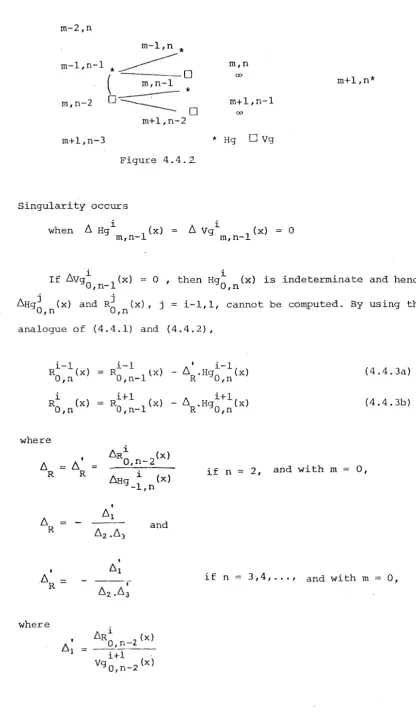
The rational interpolation algorithm The singular case

Numerical results Conclusion

REFERENCES

5. A GENERAL ALGORITHM FOR PADE APPROXIMATION TO FORMAL POWER SERIES

6.

5.1 5.2 5.3 5.4

Introduction The algorithm Semi-normal case Non-normal case REFERENCES

THE QUADRATIC APPROXIMATION 6.1

6.2

Introduction . • . . . . Quadratic approximation

6.3 Identities among the polynomial coefficients of the quadratic approximation

6.4 The general algorithm for the polynomial coefficients of the quadratic

approximation

80 80 82 90 98 107 118 119

121 121 123 128 130 131 132 132 133

135

sequences

6.6 Quadratic interpolation and

6.7 6.8

extrapolation . . . . 6.6.1 Interpolation 6.6.2 Extrapolation Numerical examples Conclusion

REFERENCES

7. SOME PROPERTIES OF THE QUADRATIC APPROXIMATION AND COMPARISON WITH OTHER NON-LINEAR

TRANSFORMATIONS . . 7.1

7.2 7.3 7.4

Introduction The properties

Numerical test results Conclusion

REFERENCES

157

162 162 170 173 186 188

ABSTRACT

This thesis is a study of quadratic approximation and its application to the acceleration of slowly converging sequences arising, in particular, from the numerical integration of an

(improper) with singularity.

It commences by considering the convergence of the

quadrature approximants to the integral with singularity. The location of singularity affects the rate of convergence when the process of ignoring the singularity is used. Numerical results show that most of the quadratures can cater for the integral with a singularity located at the end points of the interval (or subintervals) of integration.

Then the rate of convergence is considered. A number of accelerators such as the Romberg method, Aitken ~2 process and

1.

the £-algorithm are compared. The £-algorithm is not as good as the modified Romberg method, but better than the unmodified Romberg and Aitken ~2 process.

Since the £-algorithm is based on the use of the Pade approximation, a general algorithm for the calculation of rational approximations is developed.

(Muhlbach-Neville-Aitken) algorithm which can be applied to the rational interpolation and Pade approximation. This approximation can be applied to speed up the convergence of a converging sequence and can be extended to the interpolation. With the general recursive algorithm, all possible quadratic approximants and interpolants can be constructed.

The use of the quadratic approximation for linearly convergent sequences, monotonic and alternating series is illustrated. Numerical results show that the convergence of a suitable quadratic approximant is faster than Pade approximant if convergence of the Pade

3.

INTRODUCTION

This thesis is mainly a study of quadratic approximation and its application to accelerating the convergence of a converging sequence. The quadratic approximation is an extension of Pade approximation. The research is motivated by attempting to find an effective method for evaluating an integral with (integrable)

*

singularity and an effective acceleration process for

the convergence of a sequence of quadrature approximants to the integral with singularity. Such integrals often cannot be readily handled by ordinary numerical quadrature. A number of methods have been developed to deal with an integral with

singularity. These methods can be classified by three different approaches:

(i) Transform the integral with singularity to a proper integral (i.e. with no singularity).

(ii) Modify a classical technique for evaluating a proper integral to the case where a singularity occurs.

(iii) Ignore or avoid the singularity. 'Ignore' means whenever the singularity appears, the function value assigned is

zero and 'avoid' is using a numerical quadrature which does not involve the singularity.

An investigation of the process of ignoring the singularity is discussed. This process was proposed by Davis and Rabinowitz [ 2] in 1965. Since then, a number of papers on ignoring the singularity in numerical quadrature have been published. These

include the extension and generalization of this process and the study of the nature of the singularity.

A careful study of the location of the singularity appears to have been overlooked and this is discussed in Chapter 2. It is found to affect the convergence of numerical integration. Numerical quadratures which include conventional quadrature rules such as the trapezoidal rule, Simpson's rule, Gaussian rule, and others favour the integrand with an endpoint singularity. The convergence to the exact value of the well behaved integrand with endpoint singularity is monotonic. Some quadratures may give slow convergence. However, the rate of convergence can be accelerated by extrapolation processes. A discussion and

comparison of various extrapolation techniques, for example, the Romberg method, Aitken process and the E-algorithm are

three.

It is known that the modified Romberg method, applied to a function with an endpoint singularity, is an efficient procedure but at the cost of knowing the appropriate error

for the quadrature. The s-algorithm, which does not require the user to supply these parameters, is not as good as the modified Romberg method, but gives substantially better results than some other extrapolation processes such as the unmodified Romberg's method, Aitken 62 process and rational extrapolation. Much research comparing the extrapolation processes to various functions has been carried out in recent years.

5.

Starting from a study of Pade approximation, an attempt is made to extend the E-algorithm, which is the application of the well-known Pade approximation. There has been some recent interest in the generalization and extension of Pade approximation. The generalization of the two dimensional Pade approximation to three dimensional quadratic approximation was considered in Fade's

manuscript [4] in 1892, but it was not developed until 1974 .Shafer [3] considered this idea and showed the advantages of employing quadratic approximation applied to some

-1 -1 -1

particular examples such as tan x, cos x, sin x, log(l+x) and Since then, the approximation has been used in approximating experimental results in physics and chemistry. In contrast, very few studies concerning the structure and the

method of derivation of this type of approximation were then known. The work has resulted from attempts to study these

In this study, the structure, derivation and application of the quadratic approximation have been investigated. Since it is a higher dimensional extension of Pade approximation, i t has similar basic structure and common properties, but the increase in dimension leads to a more complicated computation. It is found that the generalized MNA (Muhlbach-Neville-Aitken)

algorithm by B:rezinski [ l] can be extended to the computation of quadratic approximations. This algorithm not only can be applied to the general interpolation problem, orthogonal

Chapter four extends this algorithm to rational interpolation and Chapter five extends this algorithm to Pade approximation. These form the basis of a further extension to quadratic approximatioQ

With this preparation, Chapter six concentrates on

developing the quadratic approximation. This includes the general form of polynomial coefficients of the quadratic approximation to a function f(x) which can be expressed as a formal power series. The algorithm for constructing this approximation is derived and the approximation is applied to the acceleration of the

convergence of sequences. It is essentially a generalization of the E-algorithm based on the Pade approximation. Moreover, the idea of interpolation by quadratic approximation is also

introduced and the same general algorithm can be used to calculate an interpolatory quadratic approximation.

7.

REFERENCES

1. C. BREZINSKI, The Muhlbach-Neville-Aitken algorithm and some extensions,

B.I.T.

20, (1980) 444-451.

2. P. J. DAVIS and P. RABINOWITZ, Ignoring the singularity in approximate integration,

SIA14

J.

Numer.' AnaZ.

2,

(1965) 367-382.

3. R. E. SHAFER, On quadratic approximation,

SIAM J. Numer. AnaZ.

2, (1974) 447-460.

4. H. PADE, Sur la representation approchee d'une fonction par des fractions rationelles,

Ann. Sai. EcoZe Norm. Sup.,

LOCATION OF THE SINGULARITY IN NUMERICAL QUADRATURE

2.1 INTRODUCTION

A number of methods have been found for the numerical integration

of functions with integrable sipgularities. These include proceeding to the limit, changes of variable, elimination of the singularity by

sub-traction, use of integration formulas which absorb the singularity into a fixed weighting function (e.g. Gauss type), avoiding or ignoring the singularity. For further references see [2].

Davis and Rabinowitz· [1] investigated the process of

ignoring the singularity in numerical quadrature. They show that i f the singularity occurs at a rational point and if the integrand is monotonic in a neighborhood of the singularity, then ignoring the singularity is a theoretically valid process for a large class of sequences of composite rules. Rabinowitz [12] extended the class of composite rules to include those based on quadrature formulas with algebraic nodes. Miller[8] replaced the assumption that the

integrand is monotonic in a neighborhood of the singularity by a more general condition that the integrand can be dominated by a monotonic, integrable function, A few years later, Rabinowitz [13] generalized the results so that the weigh~in the quadrature formulas are not required to be positive nor the abscissas to be rational or algebraic,

9.

that the convergence to the exact value of the integral is then

monotonic, though the convergence may be slow. Hence the assumption that the singularity is rational can be dispensed.

In the next section, a brief description of the results given previously in

[1],

[S)'and

[12],

and the necessary condition of

Theorem 2 in [l] are given. This condition leads to a way of allocating

th~ sing~larity which is discussed in section 2.3. In section 2.4

it can be shown that the integrand with singularity will converge

monotonically if one takes care of the location even if it is irrational. Some of the results of the examples in [1] are modified by using

this technique in section 2.5.

The theorems about the numerical quadrature monotonic

increasing functions with a singularity in the interval of integration whose converges have been found in

[1],[12]

and

[13}.

Let f(x) be a nonnegative and monotonic increasing function in the interval [O,f;)i; 1 with a singularity at .;, with f(x)

=

0 in the interval (.;,1], and such that

I f "

J

1

f(x)dx is finite, 0

m

Let Q(f) =

L

W,f(x.) be a simple integration rule such that i=l ~ ~

m

w.>o, Iw.

~ i=l ~ 1, 0 <Xi < X2 < ••• <X m < 1 •

A composite rule Q (f) of mn points which is based on applying Q(f)

n

Q (f) = n

n-1 m i xk

I I

wk f (- + - ) (2.2.1)

i=O k=l n n

For each integer n ~ l, define s(n) as the abscissa among the mn abscissas of Q (f) which is closest to s from the left so that

n

With these definitions, the following results have been shown in [1].

(a) (Theorem 2 in [l]) Q (f) converges to I f if and only if

n

(b)

lim~

f(s(n))

=

o.

n

n-+=

(Theorem 3 in [l]) If s

(2.2.2)

l , then Q (f) converges to I f . n

(c) (Theorem 4 in [ l]) I f s is a rational number (P/q) < l

and the abscissas x. are rational numbers, then Q (f) converges

1 n

to If.

(d) (Theorem 5 in [l]) Let 0 < s < _{l and suppose that s is} 1

irrational. If-~ a < l and f(x) is defined by

2

-a _~X

< s f(s-x) for 0

f (x) =

l

for s ~X ~l

0

Then Q (f) does not converge to I£.

n

(e) (Theorem 6 in [l]) If s is an irrational algebraic number and let 0

<a<~ where f(x) is defined as in (d).

Then Q (f)

2 n

converges to If. These results have been extended [12] in two ways, i.e.,

(f) (c) has been shown to hold for any Q in which the abscissa x. l

11.

(g) If ~

=

1, the quadrature rule Q been extended to a Gaussian

(h)

quadrature rule of interpolatory type.

In fact, it has also been extended to include the quadrature formulas of maximum algebraic with the abscissas x.

1.

being the zeros of the Chebyshev polynomial of the first and second kind in [6] .

Instead of assuming f(x) monotonic near x

=

~' Miller[8] gives a more condition for f(x). (Note that Niller's

formulation is retained in order to compare the results directly. Thus ·the non zero part of the function is taken on the right side of the singularity in this case.

Let f (x) E Md (s)

where

r!l(t;)

={f E c(t;,l]I1Ldt;,l)i f=O on

[o,t;],

f O, f non-increasing on (~,1]}

and {f E

c

(S,1]

3

F E M (

t; )

3

I

f ( t)

I

<

F ( t) on [ 0 , 1] }.

Let Q (f) =

n (J.). J.n f (X. ) 1.n 1 0 X ln < X 2n < ••• <x mn,n

<1

t which includes the previous sequence of composite rules as a

case.

'·

Robinowitz[l3] shows that

(Corollary 1 in [13]) If f E Md (s), 0

<

t;

1 and

lw. I

<

k

J.n (x. - x.

1 ) hold, where k and A are positive constants J.n 1.- ,n

independent of n 1,2,3 ••• and of i

=

1(1) m such that x.

n J.n

A<

1. Then Q (f) converges to If if and only if

n

limwkn f(~(n))

=

0 _{where s(n) is the abscissa xkn in Qn}

n-J-<)0

satisfy X

k-1,n

t;

< xkn

.

(i) (Theorem 2 in [13]). If l; is a rational number CP/q) < 1 and f(x)E Md(l;), then Qn(f) converges to If.

Note that in (h)and (i) the weight cu. need not to be positive ln

and the abscissas x. need not to be rational or algebraic. ln

(j) (Theorem 3 in [13]). If l; is irrational,O < l; < 1 and define f(x)

f (x)

E M(f;) by

J

(x-l;) y jlogj3 (x-l;)

I

1.

0

where -1 ~y ~ 0 and Sis arbitrary. conclusions hold:

The following

( i) For -1 < y < - 1

2

and all

8

and for y - -1 2 and S ;;;:. 0, no rule Q (f) converges to If.

n

1 1

(ii) For y = - -₂ and 0 > 8 ~--2 I Qn (f) does not converge to If. (iii) For y =--and 1 ₈ <--and for 1 1 < y ~ 0 and all 8,

2 Q (f)

2 2 n

converges to If for almost all l;.

Result (a) is the fundamental theorem for the other results. The necessary and sufficient condition (2.2.2) in (a) is the key of the convergence. In order to satisfy this condition, the singularity needs to be located at an end point of a subinterval. Davis and Rabinowitz [1] concentrate on the nature of the singularity and seem to overlook this point. With this condition the statement of Theorem 2 in [1] is completed. The modification of proof of Theorem 2 in

(1]

is given below.

Proof. To show if lim if(s(n)) = 0, then 1 n-+<x>

lim Qn(f) =

J

f(x)dx.

n+oo 0

integer such that k(n)/n ~ ~(n) < ;.

Define cr. (f) J.n

m i xk

L

wk f (-r + - ) .

k=:l n n

Since f(x) 0 in E;, x ~ 1.

Q (f) n

1

=

-(cr

+

n OJ

1

=

-(o: +

n 0

Since f(x) is monotonic in 0 ~ x < ; and since wk > 0 and

Again,

1 2

1, cr ~ f(-), cr ~ f(-) etc.

0 n 1 n Therefore,

1

bymonotonicity, cr

0 ~f(O), cr1 ~f<-;:;:-> etc.

m

_ \ k (n) .

crk ( ) -_{n .}l w . f (--.: + 1 J. n n

J= Hence if w min {w

1, u~-· •• wm}, crk (n) ~ wf (; (n)).

+ •.• + f(k(n)-1)) + w

n n

J

(k(n)-l,V'n

~

f(x)dx +

~

f(E;,(n)) •

0

Combining these two inequalities, we obtain

; f (n))

-IS

f(x)dx

~Qn(f)

- Jl f(x)dx

Furthermore

Therefore

f(E;,(n))

13.

(k(n)-~/n

o Jl/n

IE;

.

~ ~

f(;(n)) - f(x)dx- f(x)dx

It follows from the above expression 1

that if

lim~

f(s(n)) n+oo n

then lim Qn(f)

=

f

f(x)dx.

n+co 0

Conversely, since

J

(k(n)-1)/n

o

<

w f(s(n))

<

Q (f)- f(x)dx

n n

0

If Qn{f)

+I:

f{x)dx

~

J:

f{x)dx, then

o

~

f(s(n))

<

f(x) f(x)dx J

s - J(k(n)-1)/n

0 0

<

Js(n) f(x)dx + Js f(x)dx (k(n)-1)/n s(n)

<

[s<n> -

kC~>-l]

f(s(n)) +

o

<

~(n)f(s(n))

- k(n) f(s(n)) +

~

f(s(n)) •

· n n

Taking the limit on both sides, then

0 lim ~ f (

s (

n) ) n

n+co

lim

~

f (Ejn))

n+oo n

But if s lies on an end point of the interval, then lim k(n)-1

s

n+co n

rk

{n)-1) /n

r

f{x)dx

and lim

f(x)dx :::: n+co

0 0

from (2.2.3)

0

i.e. 0

or

lim { !::!_ f (

s (

n) ) }

<

lim Q

(f)-n n

n+co n+oo

w lim

!

f

u; (

n) )

<

0

n n+oo

lliU.

!

f(C(n)) s as requ1re • · d n

n+co

J

(k(n)-1)/n l+im f (x} dx

n co

0

0

15.

2.3 THE LOCATION OF THE SINGULARITY

If the singularity is a rational number P/q, i t can be easily located at one of the end points of a subinterval of [a,b] by

selecting n as a multiple of q. But if the singularity is irrational, i t is not possible to divide the interval to ensure the singularity is at the end point of one of the subintervals. In order to avoid this occurrence the interval can be subdivided from ~' that is

[a, nl-1

n ~a •

1

J •••

u:-

-,i=J

n

If 0 < t,; < 1,

where n1 is the largest integer such that

, where I 1 and are given by

then

J'

f(x)dx

=

I1 +

0

r

f(x)dx and I 2

0

lim

+

x+.;

r

f (x)dx

X

1 1

Then the subintervals will be [a, - -,.;],[.;,

.;+ -] ..•

n n

n 2-1 n2

[~ + , b] where n2 is the smallest integer such that .; + - - b.

n n

I

I

~igure 2.3.1

n,-1

Note that the first and the last intervals may not be the same as the others, and they have to be treated differently in the

composite rule. In this case, k(n) can be from the largest integer to the real number in the above proof.

2 4 IRRATIONAL

For the results (d) and (j) the singularity is irrational. Hence this singularity is allocated to an end point of a sub-interval.

For (d) f(E;(n)=[ (E;- -)] - 1 -a = n a for 0 ~ x < E;

n

so 1 f(E;(n))

=

na-1

n

. 1 ~ l l't f l

S1nce - ~ a < o lows that 2

For (j) - f l (E; (n)) n

lim

n+oo

1

f(E;(n))=O

n

Q (f) -+If by (a).

n

and hence

For y>-1 and

S ::;;

0 lim

l

f(E;(n)-+ 0 and hence Q (f) +I£.

n-+oo n n

However in the case

S

> 0 the convergence is very slow and we need to have nY+l >> !logS (l)

I

for reasonable computational results.

n

If ny+l >> !logS

(~)

j,

then taking the logarithm of both sides,

(y+l) log n >>

S

_{< llog<n->f}

r

_>

y >>

S

logllog (n)

I

log n

Y »

S ·(

A-1)

where A log

I

log (n)

I

log n

17.

(2.4.1)

It can be seen that (2.2.2) very much depends on

y,S

and n in this case. When n + 00 , A+ 0 in(2.4.l)but is very slow, as can be seen in table 2.4.1.

Table 2.4.1

n A

I

I

103 lOZO

1 00 _{20 0.0878437 0.1590404} 0.0650515

2 -1.7320208 40 0.1277597 104 0.1505150 1030 0.0492374 4 -0.6601042 60 0.1405779 106 0.1296919 lO!fO 0.0400515 8 -0.0490194 80 0.1468450 108 0.1128862 lOS 0 0.0339794 1 0 0.0000000 100 0.1505150 1010 0.1000000 10100 0.0200000

As

S

gets larger a much value is needed of n before- f(s(n)) 1 n

small and hence Q (f) close to If. The in the table n

(i)

y

-

0.75

s

1

(ii) y 0.75

s

2

(iii) y - 0.75

s

3 (iv) y - 0.75

S

4

Table 2.4.2

1

·~

(i) (ii) (iii) (iv)

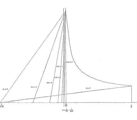
2. 5 NUMERICAL EXAMPLES

Example 1 (Example 4 in [1])

l

if x >

a

f

IX-a

f(x)dx ₁ f(x)~

0 0 if X~

_a

This integral had been approximated by trapezoidal rule T for

l l

a

= --

+ - - - and 16 - 512

1 _± 1 _{- 5 x 10} -8 _{in 1 •} [ ]

512 The results are listed below.

Table 2.5.1

~

1 1 1 1 -a 1 1 1

16 +

- -

16 + - - -5 X 10 _{16 - sT2}

512 512 16

1 1.0076 1.0076 1.0042

4 l. 3861 1.3861 1.3776

8 1.7312 l. 7312 1.7090

16 1.5785 1.5785 2.9764

32 1,6905 1.6905 2. 3728

64 l. 7731 1. 7731 2.0898

.

128 1.8375 1.8375 1.9596

256 1.8966 1.8966 1.9006

512 1.8699 29.4910 1.8739

1024 1.8888 15.6994 1.8929

2048 1.9022 8.8075 1.9062

4096 1.9116 5,3643 1.9157

exact 1.9345 1.9385

1 512 -1.0042 1.3776 1.7090 2.9764 2. 3728 2.0898 1.9596 1.9006 29.4951 15.7034 8.8ll5 5.3683

19.

From the results, we can see that for the first and third column when

n < 512, the values of n x T increase and decrease dramatically. This is

due to the contribution of the interval which lies on the left hand side of a by using T rule. This can easily be seen graphically from figure 2.5.1 - 2.5.4. But when n = 512 and beyond i t the values of n x T coverge to If gradually, since a will lie on one of the end points of the subintervals in this case.

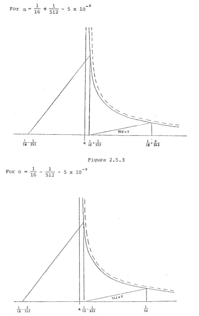
- 1 + 1 For a

-16 _ 512 right or left by 5 X 10 -8 integnant but also induces so the values of n X T

21.

1-

512 X T

'1''

Figure 2.5.2

-8

5 X 10 the singularity a shifts to the It not only contributes some values to a away from an end point of a subinterval

dramatically.

the

l

[image:26.595.88.559.87.500.2]

1 1 -8 For a

=

₁₆

+

512 - 5 x 10

I

I\

For a _{16 -}1 _{512 -}1 _{S X lQ} -8

1 2 16-SiT

I

\

\

2.5.3

[image:27.595.76.472.88.715.2]

\

23.

Now apply n x T to each subinterval which are subdivided

f rom .., , c 1. • . e • . . . [ a, '"" ~ + ~] n

1 2

[a + -, a + -] ....

n n

as below.

Table 2.5.2

~

1 1 1 -a 1 1

lG + 512

i6

+ 512 -S X 10 _{16 -}

--

₅₁₂

2 0.88668163218 0,88668168735 0. 89099027481

4 l. 20093245491 l. 20093250707 1,20500319308

8 1.41738354973 1.41738360147 1.42142147082

16 1.56920383223 1. 569 20388396 1. 57323992070 32 1.67627156897 1. 67627162067 1.68030633585

64 1. 75191782869 1,75191788039 l. 75595228300

128 1.80539229854 1. 80539335023 l. 809 42667933

256 l. 84320058152 1.84320063323 1.84723494576

512 1,86993410587 1.86993415757 1,87396846681

1024 1.88883732025 1.88883737195 1. 89287168038

2048 1.90220385110 1. 90220390280 1.90623821101

4096 1. 91165540064 1.91165545233 1. 91568976051

8192 1. 91833865143 . 1.91833870312 l. 92237301127

exact 1.934473443. 1.934473494 1.938507802

i

The results shown

1

i6- 512 + 5 X

0.8909903289 2

1.2050032451 4

1.421421'5224 5

1. 5732399722 9

1.6803063874 4

l. 7559523345 8 l. 8094267 309 1. 84 7234997 3 4

1.8739685183 8

1.8928717319 5

1.9062382626 0

1.9156898121 1

1.9223730628 6

1.938507854

_a

10

Example 2 (Example 5 in [ 1]) •

1

i f X > 0

-J:

f (x) dx

IX"

::: 2.0 f (x) ==

0 if X ~ 0

Here an integralcovBrs a range including 0 with the singularity at

o.

As mentioned in [ l ] , .for A= -0.5, this is

equivalent to a rational singularity while for the other values of A, this is an 'irrational' singularity.

For A == - 0.5 by Simpson rules we have the following results.

Table 2.5.3

n

s

n

s

16 2.06297023 24 l . 77748734 32 l . 81440591 48 l . 84265980 64 2.03148514 96 l . 88874368 128 1.90720296 192 l . 92132990 256 2.01574257 384 1.94437184 512 1.95360148 768 1.96066495 1024 2.00767129 1536 1.97218592 2048 1. 97680074 3072 1.98033247 4096 2.00393564 6144 1.98609296

Now applying S and T to n subintervals subdivided from

s

0 for other values of A.

~

-0.93727082 -0.06272918

2 1.1235524300 1.3510465951 4 1.3805514715 1.5412234050 8 1.5620068842 1.6755996258 16 1.6902936632 1.7706144828 32 1. 7810046491 1. 8377999394 64 1.8451469087 1.8853072378 128 1.8905023295 1.9188999699 256 1. 9225734545 1.9426536191 512 1.9452511646 1.9594499852 1024 1.9612867272 1.9713268095 2048 1.9726255823 1.9797249927 4096 1.9806433635 1.9856634052 8192 1.9863127931 1.9898624965

Table 2.5.5

~

-93727082 -0.06272918

2 0.52371285046 0. 92023807345 4 0.97359403996 1.24385416526 8 1. 27881361845 1. 4669436764 7 16 1. 49121007266 1.62344988396 32 1.64052427042 1.73382332040 64 1.74588585904 1.81180578698 128 1.82033164635 1.86693187740 256 1. 87295965866 1. 90590794927 512 1. 91017000566 1. 93346720149 1024 1.93648087494 1. 95295428918 2048 1.95508526425 1. 96673367944 4096 1.96824050299 1.97647716453 8192 1. 97754264860 1. 98336684456

So from the above results, i t can be seen that no matter what the singularity is, rational or irrational, as long as it is located at the right position , Q (

3 {Example 2 in [7]) :=:.;:..:.=;ce._;.;_:=:.;:..c...

I£

=I:

(x2 - 0.01)-1 dx - 1. 0033534.

a) By Trapezoidal rule.

{i) Singularity is not at the end point of a subinterval. (ii) Use 10 x n intervals where n

=

1,2, •• ~o ensure the

singularity always lies on an end point of. a subinterval. The results are given in Table 2.5.6.

Table 2.5.6

n { i) (ii}

2 -22.664141414 10 -2.949494949

4 -6.117677257 20 -1.976000608

8 20.614154589 40 -1.489570856

16 4.099809449 80 -1.246435602

32 -22.623676159 160 -1.124887898

64 -6.107221645 320 -1.064119029

128 -20.616792793 640 -1.0337 35837

256 4.100470581 1280 -1.018544553

512 -22.623510779 2560 -1.010949002

1024 -6.1071800296 5120 -1.007151231

2048 20.616803115 10240 -1.005252347

4096 4.100473154 20480 -1.004303015

8192 -22.623520283 40960 -1.003828211

16384 -6.107180172 81920 -1.003590789

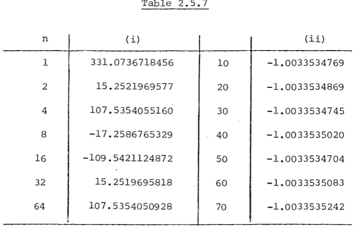
b) By eight point gauss - Legendie rule (as in [7])

Table 2.5. 7

n ( i) (ii)

1 331.0736718456 10 -1.0033534769

2 15.2521969577 20 -1.0033534869

4 107.5354055160 30 -1.0033534745

8 -17.2586765329 40 -1.0033535020

16 -109.5421124872

so

-1.0033534704

32 15.2519695818 60 -1.0033535083

64 107.5354050928 70 -1.0033535242

The results in (i) are at such variance no conclusion can be made since the singularity is not at the end point of a subinterval but (ii) gives a confident answer since the singularity always lies on the end point of a subinterval.

This technique has also been considered by Harris and Evans in (9] ;where they generalised theN- point Gaussian

quadrature to cater for end-point singularities. They suggested the choice of subintervals such that the singularity lies on an end-point if i t is internal, but they have not really extended the idea to other quadrature rules. They have essentially

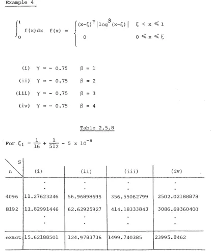
[image:33.595.118.478.152.383.2]

Example 4

r

f(x)dx f(x) 0

(i) y - 0. 75

(ii) Y==-0.75

(iii) y - 0.75 (iv) y - 0. 75

B

== 1

B

== 2

B

3

B

== 4

Table 2.5.8

1 1 8

·Far /;1 ==

16 + 512 - 5 x

10-~

(i) (ii) (iii)

.

.

.

.

.

.

4096 11.27623246 56.96898695 356.55062799 8192 11.82991446 62.62925927 414.18333843

.

.

.

.

.

_.

exact 15.62188501 124.9783736 1499.740385

29.

(iv)

.

2502.02188878 3086.69360400

.

.

[image:34.597.82.496.103.594.2]

For

~

4096

8192

exact

=

₁₆ 1 ₁₅₂ 1

(i)

.

.

11.27649708 11.830179076

.

'

15.64529233

_8 5 X 10

(ii)

•

.

56.96900403 62.62927636

>

'

125.165236

(iii)

,

.

356.55062910 414.18333953

.

,.

1501.982754

The convergence of the above integral with these

(iv)

.

"

'

2502.02188890 3086.69360400

.

24031.72407

.are shown in section 2.4 to be very slow. It is necessary that n > 103 in (i)

n > 105 in ( ii) n > 106 in (iii) and n > 1015 _{in (iv)}

31.

2.6 CONCLUSION

The original investigation of the of ignoring the singularity by Davis and Rabinowitz [l] has led to extensions and

generalizations [6] ,[8] ,[10] ,[11] ,[13], as well as studies in the rate of convergence and error bounds [31 ,[4] ,[5].

In this chapter it has been shown that the location of the singularity does affect the speed of convergence when the technique

of ignoring the singularity is applied to an integrand with singularity, whether it is rational or irrational.

work is a necessary complement to [1] and [13].

Feldstein and Miller [4] state that avoiding the

Thus, this

singularity is easier to handle theoretically while ignoring the singularity is easier to program. Rabinowitz [14] prefers to use a quadrature rule which avoids the singularity. However,

experience has shown that most of the results favour quadrature rules with an endpoint singularity.

in the next chapter.

REFERENCES

1. P. J. DAVIS and P. RABINOWITZ, Ignoring the singularity in approximate integration.

SIAM

J.

Nwner. Anal.

2

(1965) 367-382.

2. P. J. DAVIS and P. RABINOWITZ, Method of Numerical Integration.

Academic Press,

New York.

3. M.E.A. EL-TOM, On ignoring the singularity in approximate integration.

SIAM J. Numer. Anal.

8 (1971) 412-424. 4. A. FELDSTEIN-and R. K.' MILLER, Error bounds for compound

quadrature of weakly singular integrals.

Math. Camp.

25 (1971) 505-520.

5. L. FOX, Romberg integration for a class of singular integrands.

Comput

J.

lO

(1968) 87-93.

6.

w.

GAUTSCHI, Numerical quadrature in the presence of a singularity.

SIAM

J.

Numer. Anal.

4 (1967) 357-362. 7. A. C. GENZ, Applications of the €-algorithm to quadrature

problems in

Pade approximants and their Applications.

P. R. Graves-Morris, ed. (1973) 105-116.

8. R. K. MILLER, On ignoring the singularity in numerical quadrature.

Math. Camp.

25 (1971) 521-532.

33.

10. C. F. OSGOOD, Numerical quadrature of improper integrals and the dominated integral. J.

Approx. Theory.

20

(1977) 139-152.

11. C. F. OSGOOD and OSHISHA, The dominated integral. J.

Approx. Theory.

17 (1976) 150-165.

1?. P. RABINOWITZ, Gaussian integration in the presence of a singularity.

SIAM

J. Numer. Anal.

(1967) 191-201. 13. P. RABINOWITZ, Ignoring the singularity in numerical

integration.

Bk # 03005 Topics in Numerical Analysis

111, ed. John J. H. Miller (1977) 361-368.

EXTRAPOLATION PROCESSES FOR INTEGRANDS WITH SINGULARITY

3.1 INTRODUCTION

As mentioned at the beginning of Chapter 2, there are a number of methods to deal with singular integrands, f(x), where f(x) is continuous on [a,b) and has a singularity at b. The value, I of the integral is then defined by

~~

lim

I-~~

j

f(x)dx

a

(3.1.1)

and is assumed to exist.

There are different approaches to the evaluation of this improper integral. The first approach is to transform the improper integral to a proper integral. The second approach is to modify a classical technique for evaluating proper integrals to the case where a singularity occurs. The third approach is to ignore or avoid the singularity (see Chapter 2 and [18]).

Robinson [19] compared fifteen general purpose numerical integrators by using one hundred and ten test integrands from five different types of behaviour of the integrand. One type is a function with one or more singularities within the

integration interval. His results show that for those

integrators which are reliable and efficient for this type of function most failures occur for functions which have a

35.

The integrals involving endpoint singularities give accurate and reliable results. At points where the function has a infinite value these algorithms the value zero. This is

equivalent to the process of ignoring the singularity.

The next section gives a brief introduction to some of the numerical quadrature methods which deal with a singular integrand.

To improve the results, some acceleration procedure such as the Romberg method (unmodified and modified) , repeated

Aitken's ~2 process (apply Aitken's ~2 process repeatedly),

extended Aitken process, the s-algorithm or rational extrapolation may be used. These are studied in section 3.3. These acceleration processes can be shown to belong to the Neville type extrapolation. The Aitken's ~2 processes (repeated and extended) can be viewed as finding a solution to a fixed point problem. In section 3.4, this approach is extended to the s-algorithm, and can be shown to give the accelerated value with error of any order k. This chapter ends with some numerical results and conclusions.

3.2 NUMERICAL QUADRATURE FOR AN INTEGRAND WITH ENDPOINT SINGULARITY. Numerical quadrature formulas for an integrand with endpoint singularity include linear and nonlinear techniques.

inverse fourth root and inverse three fourth root endpoint

singularities. Stenger [27] [28] gives a quadrature rule which is a transformation based on the Trapezoidal formula. I t has been shown to give exponential convergence in some cases when the singularity is ignored.

For non-linear quadrature, Sidi [24] used the results of nonlinear transformations - t,u,v transformations [11] to modify numerical quadrature formulas for weight functions with algebraic and/or logarithmic endpoint singularities. He compares these with Gaussian rules and finds that they are simpler to

compute and practically as efficient as the corresponding

Gaussian rules. Werner and Wuytack [29} give techniques which are based on the use of Spline approximation and Pade

approximation. They compare these methods with some other methods and claim that they are competitive with an adaptive Gaussian

quadrature scheme.

Squire [25] [26] did a comparison of Harris and Evans' modified 10 point Gaussian rule, Stenger's quadrature and Werner and Wuytack's nonlinear techniques. He concluded that the appropriate linear quadrature can handle an integrand with endpoint singularity more effectively than the nonlinear method.

37.

of the Aitken 62 process. Werner and Wuytack [29] also give a technique for using extrapolation to improve the numerical results. This technique in fact is the same as the repeated Aitken 62 process. It will be explained in the next section.

3.3 THE EXTRAPOLATION PROCEDURES AND ASYMPTOTIC ERROR EXPANSION. A brief description of some of the extrapolation processes are given below.

(a) The classical unmodified Romberg method. If f E

c

2k+l

[a,

b] , then

" r

f(x)dx a

If

can be approximated by the trapezoidal rule

k 211

hk

I

j=Q

f( a + J 'h) ·k w ere h hk = (b-a)/2k

(3.3.1)

11

where

I

indicates that half the contribution is included from each endpoint.

k

The error, E(h,f) = I f - T

0 , can be expressed using the E ule.r-Maclaurin formula in the form

+akh2k ·+ 0 (h2k+l), h

~

0. (3.3.2) where a. are constants formed from the Bernoulli numbers and

~

the derivatives of f(x) at the end points.

0 T 1

4mTk+1 _ Tk m-1 m-1

4m - 1

m _{1, 2, ...} (3.3.3)

This can be generalized to

k

h2 Tk+1

_-

_h2 Tk k m-1 k+m m-1 T =

m _h2

_{- t2}

_.

k k+m

(b-a)/

where hk

=

nk (3.3.4)

Different sequences {nk} have been used to accelerate convergence

(2], (3].

Oliver [16] did a comparison of various methOds based on polynomial extrapolation for the definite integrals. He

concluded that for a general purpose procedure extrapolation of the trapezoidal rule, using a sequence favoured by Burlirsch [2] gives maximum accuracy.

(b) Modified Romberg method.

However, the Euler-Maclaurin summation formula for the error expansion E(h,f) (3.3.2) is not suitable for numerical computation if f(x) has a singularity. Navot [13], [14] and Lyness and Ninham [12], [15] have generalized the asymptotic expansions suitable in such case. When f(x) has a singularity at an endpoint (3.3.2) is replaced by

If al

T

2 then the use of (3.3.3) or (3.3.4) in this case gives

= O(hal) and the convergence of TO

k

rate as the trapezoidal rule T k.

0

39.

a·

Fox [5] gives an account for the h ~ terms in (3.3.5). For functions with an unbounded first derivative at an endpoint (lower limit is taken here) , he shows that the contribution to the error in the trapezoidal and Simpson's rule E (h)f and E (h)f , for

T 0 S 0

a sufficiently small interval h, comes from the lower limit in the forms

1 2 1 3 2 29 4 3

=

(U

h D

-12 h D + 720 h D . . ) f 1

1 4 3 1 5 4 2 6 5

=

(180 h D- 180 h D + 945 h D . . . )fl

(3.3.6) (3.3.7)

where Di is the ith derivative of f(x). These terms then added to the usual series of powers h2 , h4 , h6 .. for trapezoidal rule and h4, h6 , h8 .. for Simpson's rule respectively which are derived at the upper limit if the integrand is completely well-behaved except at a. For those functions with a singularity in the integrand at one or both endpoints, Fox prefers a formula which does not include these points. He proposes the use of composite midpoint rule and the term embodied in the error is

(3.3.8)

together with the standard even powers of h if the function is

well-behaved. 1

For example if I "

J

0

xtdx, then

I - T (h) a

1

~h

+ a2 h2 , + a3 h4 + ...

Shanks [23] gives a simple and economic technique to eliminate these lower order terms in this error expansion.

It is equally applicable for more complicated error terms with repeated occurrence of the £n h term. For example,

I f I = - ( x

l><

3x dx then

I - T (h)

=

ah 2 + bh 2£nh + ch 2£n;. + dh2£n3:h

4 6

+ eh + fh + · · ·

The error terms can be eliminated by using the modification of (3.3.3)

2Cim - 1

with a

=

2, 2, 2, 2, 4, 6,. • .

m

(c) Aitken's process.

(3.3.9)

If a is not known, Werner and Wuytack [29] suggest that

m

these can be approximated numerically. Assume an expansion of the form

00

I - Q(h)

₌

I

i=O

eli a. h

l (3.3.10)

where Q(h) is an approximation for the integral I in (3.1.1) Consider Q(h),

Q(~)

and

Q(~).

and the a. and

a.

are unknowns.

l l

a

₀ can be approximated by h

- Q(h)

ao

Q(-) 2

2

=

Q(~)

h

- Q(-)

41.

Then I

This is the well known Aitken's 62 process which uses three successive estimates to eliminate the lowest order term in the error. When

a

0 is found, a similar technique can be used to find a l'a 2 ... ; that is to apply Aitken's 62 process repeatedly.

(cl) Repeated Aitken's 62 process.

The Aitken's 62 process, used on the converging sequence {x.}, can be considered as the iteration

].

~ (x.)

].

which converges to a solution x =X of a function f(x) = ~(x) - x 0. Let the error in x. be E ..

]. ].

x

=

X + E.

i ].

Suppose ~{x) is analytic around X.

and X·

1

where E 1

~ (xo) X + a

1E0

~ (xl) X + a

1E1

and ai = ~ i (X)

I

i ₁

+ a E_{2 0} 2 + a E3 +

3 0

2

+ a2El + a E3 +

+ a E3

3 1 3 1

+ ...

...

...

Then

Convergence is then assumed if I~' (x) !<1 in some neighbourhood of X, which implies la1 !<1.

Combining these three first order approximations and x

2, a second-order approximation, x 12, is obtained

X '

0 X

with an asymptotic error constant

~2 1-a

1

and the Aitken value

~2

=

2x -x -x 1 0 2

=

where !Jx

0 X - x and A

2_{x x 2x + x}

1 0 u 0 2 - 1 0

Using the same process repeatedly, the Aitken values can be obtained column by column and can be written in the following array

X O,l X

x1,2 1,1

X

x2,2 _x2,3

2,1

X

x3,2 3,1

X

4,1

where {x.

1}

=

{x.} i

=

0,1,2 •..

~, ~

where

Figure 3.3.1.

This repeated process can be expressed in the form

=

xj1,k

-xj+1,k- 2xj,k + xj-1,k j

xj+1,k- dk+1 xj,k

j

1 - dk+1

x.,~ 1 k - x. k

__,+ , J,

X - X

j,k j-1,k

(3.3.11)

(c2) Extended Aitken process.

Overholt [17] observed that any first-order

approximation gives a second-order formula and he extended the Aitken's ~2 process in the following way.

Suppose that the first k+1 members of the sequence {x.}

]:

used in a certain function, ~k' to give an X-approximation of order k. Then

X

l,k ~ k (X Orlr lr X 1 • • • • X k,l )

k k+l

= _{X+ ak,kEO + ak+1 ,kEO ...}

The next value is

where

X

2,k

k

El

X + _{ak,kE 1 + ak+1 ,kEl} k k+1 _{· · ·}

a lkE Ok + k k-1a E k+1

' \ '2 0

where akk =j= 0

Then the accelerated value x of order k+1 is J.,k+1

X = X

l,k+1 _{2 ,k}

a k

1

+ (x . -x )

1_a k 2,k l,k 1

where a1 can be approximated by

The array is the following xO,l

X X X X

lrl 1r2 lr3 1;4

X X X

2,1 2r2 2r3

X X

3 ,1 3,2

X

4 ,1

Figure 3.3.2

.

and k E.

J

+ ...

The recursive formula can be written as

where

X

-j+1,k

1 - {dj ) k

k+1

X - X

j+k,1 j+k-1,1

X - X

j+k-1,1 j+k-2,1

(d) The £-algorithm.

(3.3.13)

(3.3.14}

(3.3.15)

An important generalization of (c) known as the £-algorithm is due toShanks [22] and Wynn [30].

The fundamental relationship of the £-algorithm is

{3.3.16)

In applications, this relationship is rearranged to give

with Ej = 0 j

₌

1,2 -1

Ej ₌

x. 1 j 0,1

b J I

where x.

1 is a member of a slowly convergent (or divergent) J,

sequence. Th e approx1man o . t f xj,l 1s g1ven Y . . b £j

2k. The

(('j-1- ('j )-1 _{~2k ~2k +} ( j+1-_E2k , j _G2k )-1 ₌

with E: j 00 -2 and E:j X,

0 _J (E:j+1

2k-2

for k 0,1,2, .. .

j = 1,2,3, .. .

E:~

can be set out in the array shown in figure 3.3.3.

so

0

E: 1 E: 0

-1 1

E:l so

0 2

E: 2 E: 1

-1 ₁

E: 2 s l

0 2

E:

?

E: 2

-1 1

€3 0

Figure 3.3.3

45.

(3:3.17)

If 2n+1 x. s are given, with k constant for the column? J

and j constant for the upper diagonals, then the sequences

E:~

(j = 0,1,2 ... 2n),

E:~k(k=0,1,2

... (2n-2)) successively give

better results than {x.}.

J The convergence and stability

of this algorithm can be found in [31]. j-1 Macdonald [20] showed that E

2k+l can be expressed in

j-1 j j+1 j+1 j

terms of E₂k , E₂k, E

D j-1 G j-1

j-1 2k+2 _E:j

+ ( 2k+2

)

E:2k+2 j-1 j-1 2k (3.3.18)

l+G2k+2 1 + G _2k+2 where

( j+l - E:j ) 2

j-1 j+l E:2k 2k

0

2k+2

=

E:2k j+l _{- 2E:j +} j-1 E:2k _2k E:2k

(3.3.19)

and j-1 G2k+2

=

. j+l (E2k-l

j . j-1 E2k-l) (D2k+2

j

- E:2k) (3.3.20)

j-1 j-1 j-1

where G

2k+2

=

0,(3.3.17) shows that

s

2k+2

= n

2k+2 which reduces to the Aitken's 62 process (3.3.11). (3.3.18) can be rearranged

. j-1 j

in terms of the elements in the even column, 1.e., s

2k , s2k'

j+l j+l

s

2k and s2k_2, can be expressed by a similar expression to

(3.3.11) and (3.3.14). This gives another expression of (3.3.17). S ;nce Dj-l _~ · th A'tk ' A2 ' t b ' t t

2k+2 1s e 1 en s u process, 1 can e wr1 en as

where

j-1 0

2k+2

dj+k 2k+2

j+l dj+k j E:2k 2k+2 E:2k

1 - dj+k 2k+2

Then substitute the above expression into (3.3.18) j+l -j+k j

j-1 E:2k - d2k+2 E:2k E:

2k+2

-j+k 1 - d

2k+2

where -j+k = dj+k - (1-dj+k )Gj-1 d2k+2 2k+2 2k+2 2k+2

j-1 Substituting for G

2k+2 from (3.3.19) and (3.3.20) gives

4 7.

-j+k _dj+k j+l j j+l j

d2k+2

=

_2k+2 (E:2k-1 E:2k-1} (E:2k - E:2k)

If _E:2k-1 j+l _{- E:2k-1} j =f 0 then from {3.3.16} 1

j+l j

-j+k dj+k E:2k - E:2k d2k+2

=

2k+2 j j+l

E:2k E2k-2

j-1 j+1

E:2k _{- E:2k-2 dj+k} j j+1 2k+2 E:2k

-

E:2k-2

(3.3.22}

Since the even columns E;k give the accelerated values of {xj, 1} it can be written as

k

=

1,2 ..•

j == 0,1,2 ...

Then (3.3.21) can be expressed as

xj+k,k+l

=

-j+k

X, _{]+ +} k 1 k - d X, k k

I k+l ]+ I

1 - d-j+k

k+l

and this can be simplified to

k

=

1,2 ..•

j

=

0,1,2 ...

-j

xj+1,k- dk+l xj,k

k

=

1,2... (3.3.23}

- j

1 - dk+l j

=

k,k+l. ..

where

₌

x. J + , 1 k - x. J, k xj,k- xj-l,k

(e) Rational extrapolation.

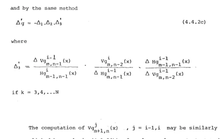
Bulirsch and Stoer [3] developed a nonlinear method for accelerating the convergence of a sequence Q(h) (3.3.10). The approximant Q(h) of I is now approximated by a rational function Ri (h) .

]l,V For an expansion in terms of h 2

i i 2 aih2].l Ri (h2) ao + a1h

+ +

= 11

]l,V

bi + bih~ + _{+ bih2\)}

0 1 \)

The recursion formulas analogous to (3.3.4) are rather

complicated, but can be simplified by choosing 11~ [m/2 ] and \)

=

_m

-

_{[m/2] and writing Ri}

=

Ri.

].l,V m In this case the formulas

become

Ri+1 "

.

i i m-1

-

dl R m m-1 R

=

m _"· (3.3.25)

1

-

dl m with R i 0

-i i

=

Q(h.).

Ro _l

"'· h. 2 Ri+1

-

Ri+1

where dl

=(

1+m) m-1 m-2

i '+1

m h. _Rl

l R

-m-1 m-2

(3.3.26)

An algorithm for generalized rational extrapolation will be given in the next chapter.

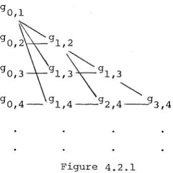
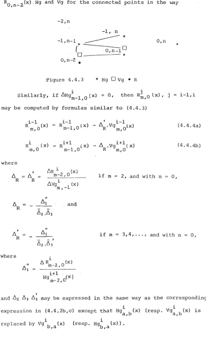
[image:53.598.85.490.150.559.2]

49.

n g(h) g

c

0) +

I

m=l

a e (h)

+

R (h)

m m n (3.3.27)

where (h) j

=

1,2 ... are known functions satisfying lim e m+ 1 (h)

0

=

h-+0 e (h) and R n (h)

=

O(e n+ 1(h)) is the error term.

m g(O)' a a ... a

1' 2 n are unknowns and g(h) can be calculated for a

sequence of steplengths h

0 > h1 > h 2 > •••• >0. The unknowns a,, a •.. a can be eliminated successively by computing the

.L 2 n

lower triangular table

gO 0 gl

0

gO 1

g2

0

gl

1

gO 2

Figure 3.3.4

With the elements defined by Neville's algorithm g t+1 - dt Qt

t m-1 m m-1 Q

=

---;:---m 1 - dt

m > 0 (3.3.28)

m

and starting with

Q~

=

g(ht) where the extrapolation coefficients dt are defined by

m

E £+1 d 9.,= m-1,m

m E £

m-1,m

(3.3.29)

with EQ,

=

e j (hQ,) • QQ. is related to Q (O) through the expansion

Q,J m

QQ.

₌

_{Q(O) +} n

_I

_a, EQ, ₊ RQ, m

j=m+l J m,j m

The error elements satisfy the Neville's algorithm if the Q-elements are replaced by the R-elements with

R~

=

Rn(hQ,) •

Comparing the elements QQ., which are obtained from the

m

extrapolation processes (a} - (e), to the expansion (3.3.27), we note that they have a recursive relation similar to (3.3.28)

(3.3.30}. It is well known that (a) and (c) are of this type. The extrapolation coefficients dQ, can be obtained from (3.3.29).

m

(e) is similar to this type but the extrapolation coefficients dQ, are approximated by nonlinear transformation (3.3.24).

m

For (a) and (b) , two successive terms in a column are needed for extrapolation in (3.3.3) and (3.3.4} provided dQ,

m

is known. If dQ, is not known, for example (cl), a third term

m

is needed in the same column in (3.3.11). For (c2) , since the

Q,

approximation of d based on its first approximation three

m

successive terms are needed to give the first approximation of dQ, in the first column; the rest need only two successive

m

terms (see (3.3.14)). For (d) three successive terms in a column and a term in the preceding column are needed and

51.

3.4 COMPARISON AND ERROR ANALYSIS OF SOME EXTRAPOLATION PROCESSES The comparison of the extrapolation processes (a) , (b) 1 (c1) and

(d) and the comparison of (a) 1 (d) and (e) are given in [4] and

[10] respectively. Their conclusions are that for well-behaved integrands, (a) and (e) give reasonably effective results. For functions with endpoint singularities (b) gives the best results provided all the exponents in the asymptotic error expansion are known. Otherwise (c1) gives better results than (a) and (e) . In the case of functions with logarithmic endpoint singularities, the error expansion is more complicated and (d) gives better results than (cl) but not as good as (b).

The extrapolation processes (cl) , (c2) and (d) can be considered as finding a solution to a fixed point problem, i.e., considering x. k as a function of x.

1 k

1 1 1 - 1 x. 1, k

=

¢k (xi_

1 ,k> , a one-point iterating function of order k with the asymptotic error constant ak,k given. Overholt [ 17] gave the (k + 1)th order approximation x. k

1 of X by the J, +

extended Aitken method (3.3.13) with an asymptotic error constant

k

a ak+l ,k+l

=

This expression appears to be in error and should be expressed as

ak+1,k+1

=

k-1 a

l k

1-a

1

- j

Since from (3.3.15} dk+l (denoted as Tj+k in [17]) can be expanded in terms of a 1 via (3.3.13}.

-j

dk+l is the first order approximation of al with k-1

C/,1

=

(1 + a

1) a 2'

Substituting this and (3.3.13} in (3.3.14) gives xj,k+l

with ak+l,k+₁ which is given by (3.4.1}.

The repeated Aitken's

6

2 process, extended Aitken process and the s-algorithm give the same approximation x.

2 where j

=

1, J,

2 •.• on the second column of their arrays (Figure 3.3.1-3.3.3).

2 3

X, 2 = X + a22 E. 1 + a E. 1 + (3.4.2)

J, J- 32

J-2 with

l+a

1 2 l+a1 a22 :::: a32 - a 3 ₁ - a ₂ {1-a ) 2

l

Using (3.3.11), (3.3.14}, (3.3.21) and (3.4.2) again, i t

follows

3

2, 3, ...

X. 3 = _{X + a33 Ej-2 +} j

J, ₄

with _a33 = { 2al3a2 _{1-a 2{l-a 1 -} a 2) _{a 22 - 1+a.}

a~

} 1'32 a 1

. 1 l

a 4a 2 _l-3a 5

c-

La

2 1 al a3

extended Aitken

= _{+ '1-a ) a for} process

l 1-a1 1 1

3 4 (3.4.3)

(-

2a1 a2 al

₎

1

a33 = _1-a 2~ a 22 + - · - a _l+a 1 32 4 21 5

a 1 a2 al a3 ₁

62

::::

(1-a -

J:=a-)

for repeated Aitken's process

l 1 1

53.

1

for the £-algorithm (3.4.5) Hence these three processes give an approximation x.

3

J r

to X of order three with slightly different coefficients a 33. Now the same assumption is made as in the extended Aitken process.

k th column of obtained by the

x. k fork= 2,3, ... , j

=

k-l,k, .•.. is the J,

the approximation of {x.

1} j 0,1,2, •.. J,

I

repeated Aitken s ~2process and the

E: -algorithm. Assume that these x. give an X approximation

J ,k of order k+l.

Write

X. l = X + E. j = 0,1,2,

J I J

where

2 3

al Ej-1 + a2Ej-l + a3Ej-l +

.

.

.

and

E k+l k+2

= X+ a _{k+l,k+l j-k} +a _k+2,k+ lE. _J-k +

for k = 1,2, . . j

=

k,k+l, (3.4.6) Then by (3.3.11) and (3.3.12), using the same method as in deriving (3.4.1)

by (3.3.23) and (3.3.24)

a

k+1,k+l

2

a

k-l,k-1

for repeated Ai tk.en' s 6.2 process. ( 3. 4. 7)

It is not easy to tell which one is better without knowing some information about the iteration function of the given sequence. From numerical experiments, the repeated Aitken's ~2 process is better than the extended 62 process. The €-algorithm

is probably the best. In some cases such as an oscillating sequence, some of the columns obtained from repeated Aitken's ~2 process

are slightly faster than the £-algorithm, but the £-algorithm will catch up later.

3.5 NUMERICAL RESULTS

The approximation of the following integrals with endpoint or the first derivatives with endpoint

singularities are•approximated by Trapezoidal rule T (ignoring n

the' singularities) then accelerated by (i) Modified Romberg method (ii) extended

l

process (iii) repeated

t:/

process and

a)

x-~dx

=

2.

n

1 0.957106781

2 1.267228525 2.015928645 4 1.483036302 2.004042364 8 1.634748652 2.001014665 16 1.741802668 2.000253925 32 1.817445514 2.000063499 64 1.870919134 2.000015873 128 1.908727207 2.000003970 256 l . 935460679 2.000000990 512 1.954363881 2.000000248 1024 1.967730409 2.000000062 2048 1.977181958 2.000000016

Table 3.5.1

(i)

2.000080271

2.000005432 2.000000443 2.000000346 2.000000006 2.000000023 2.000000002 2.000000000 1.999999996 2.000000002 2.000000002

l . 999999996 1.999999996 2.000000000 2.000000001 2.000000000 2.000000000 2.000000000 2.000000000

----..

2.000000000 2.000000002 1.999999996 2.000000002 1.999999996 2.000000001 2.000000000 2.000000000

2.000000002 1.999999996 2.000000002 1.999999996 2.000000001 2.000000000 2.000000000

•

1 0.957106781

2 1.267228525 1. 976844358 4 1.483036302 1.993848173 8 1.634748652 1.998430296 16 1. 741802668 1.999604923 32 1.817445514 1.999900996 64 1.870919134 1. 999975242 128 1. 908727207 1.999993796 256 1. 935460679 1.999998456 512 1.954363881 1.999999615 1024 1.967730409 1.999999904 2048 1.977181958

2.010462398 1. 998918565 1. 999796713 2.002974548 1.999577822 1.999980979 2.000776093 1.999880295 1.999998468 2.000196760 1.999968936 l . 999999757 2.000049462 1.999992053 2.000000072 2.000012348 1.999998067 1.999999966 2.000003116 1.999999491 2.000000005 2.000000773 1.999999876

2.000000193

2.000020485 2.000002222 2.000000034 2.000000140 1.999999943 2.000000013

1.999999615 1.999999722 2.000000155 1.999999915 2.000000023

U1

n

1 0.957106781 2 1. 267228525 4 1.483036302 8 1.634748652 16 1. 741802668 32 1.817445514 64 1.870919134 128 1.908727207 256 1.935460674 512 1. 954363881 1024 1.967730409 2048 1.977181958

----··--·-·--1. 976844358

1.993848173 2.000120554 1.998430296 2.000009838 1.999604923 2.000000772 1.999900996 2.000000093 1. 999975242 1. 999999978 1.999993796 2.000000019 1.999998456 1.999999998 1.999999615 2.000000000 1.999999904

· ·

-(iii)

1.999999964 2.000000038 1.999999954 2.000000008 2.000000005 2.000000000

1.999999999 1.999999987 2.000000005 2.000000014

U1

-..]

1 0.957106781

2 1. 267228525 1.976844358 4 1.483036302 1. 99384817 3 8 1.634748652 1. 998430296 16 1.741802668 1.999604923 32 1.817445514 1. 999900996 64 1.870919134 1.999975242 128 1. 908727207 1.999993796 256 1. 935460679 1.999998456 512 1. 954363881 1.999999615 1024 1. 967730409 1.999999964 2048 1. 977181958

2.000044468 2.000003007 2.000000165 2.000000039

1. 999999973 2.000000189 1.999999998 2.000000000

1. 999999950 2.000000033 1.999999899 2.000000000 2.000000004 2.000000000

1.999999996

1. 999999997 2.000000004 2.000000002

(.}1

ro