Torsion dependence of the critical current in a superconducting Nb3Sn wire: modeling versus experiment

1

TORSION DEPENDENCE OF THE

CRITICAL CURRENT IN A

SUPERCONDUCTING NB

₃

SN WIRE

3

BSc. Thesis Advanced Technology Energy, Materials and Systems, Faculty TNW

University of Twente

August 22, 2013

Author: Committee:

M.L.R. van den Baar Dr. M.M.J. Dhalle

Ing. R. Pompe van Meerdervoort Dr. H.K. Hemmes

4

Abstract

In large magnets, mechanical forces on the wire rise very high. These forces may degrade the superconducting performance of the wire. The impact of the forces depends on the wire structure. Extensive research has been done on axial and transverse deformations of single strands, but not on torsional deformation. The research in this thesis is an addition to the understanding of the strain sensitivity of the critical current in superconducting . The first result of the effect of torsion on a

5

Table of Contents

Abstract... 4

1. Introduction ... 6

1.1 Superconductivity ... 6

1.2 Superconducting materials ... 8

1.3 Mechanical loads and strain scaling behavior ... 8

1.4 Parallel magnetic field... 12

1.5 Course of the assignment and lay-out of the thesis ... 13

2. Modeling ... 14

2.1 Structure... 14

2.2 Calibration ... 15

2.3 Results and discussion ... 17

2.4 Conclusions ... 19

3. Experimental details ... 20

3.1 Configuration and setup ... 20

3.2 Materials and Methods ... 22

4. Results & discussion ... 25

5. Conclusion ... 33

5.1 Main conclusions ... 33

5.2 Recommendations ... 33

6. References ... 35

7. Appendices ... 38

Appendix A ... 38

Appendix B ... 40

6

1.

Introduction

The research in this thesis is an addition to the understanding of the strain sensitivity of the critical current in superconducting . The first result of the effect of torsion on a bronze route strand is obtained in parallel magnetic field.

Superconductors are being used as powerful electromagnets, for instance in MRI machines, particle accelerators and experimental fusion reactors. To understand the performance of a superconductor, research is being done regarding the influence of external factors on the performance of the material. The influence of strain, temperature and magnetic field on the critical current is extensively researched. From these results scaling laws have been proposed to describe the critical current dependency on strain, magnetic field and temperature ( .

In large magnets, mechanical forces on the wire rise very high. These forces may degrade the superconducting performance of the wire. The impact of the forces depends on the wire structure. Extensive research has been done on axial and transverse deformations of single wires, but not on torsional deformation.

1.1

Superconductivity

Superconductivity was first observed by Kamerlingh Onnes[1]. He first liquefied helium and thereafter it was possible for him to observe the superconductive state in mercury.

A material is in the superconducting state when the electrical resistance is zero. Electrical resistivity originates from the scattering of electrons on thermally excited ions. Therefore, the lower the temperature is, the lower the resistance is. With zero resistance no power is dissipated. Therefore the materials are favorable to be used for generating strong magnetic fields. This is because strong magnetic fields are generated by high electrical currents, and high currents in a normal resistive material dissipate a lot of power. Momentarily these magnet systems are used in the ITER project, which focuses on producing energy from fusion.

Not all materials are superconductors. Most materials have a remaining electrical resistance at zero Kelvin. This is also the main issue in superconducting technology: current superconductors are only in the superconducting state at relatively low temperature, i.e. in this thesis in the order of a few Kelvin. In this paragraph an introduction is given on superconductivity.

A superconductor is only in the superconducting phase within certain boundaries. These boundaries are determined by the critical temperature ( ), the upper critical magnetic field ( ), the critical

current ( ) and the strain state ( .

When temperature descends below the critical temperature, electrons find it energetically preferable to form Cooper pairs. These cooper pairs are responsible for the superconducting state [2]. The binding energy of Cooper pairs serves as an energy gap that also describes the critical temperature. This is because the energy gap is larger at lower temperatures and it vanishes at the critical temperature of a superconductor. The critical temperature is the temperature at which a material changes from a superconductor to a normal resistive material.

7

resistive state. To explain this any further it is necessary to explain some things about flux pinning, fluxoids and type II superconductors.

There are two types of superconductors, type I and type II. Type I superconductors are characterized by the Meissner effect, or in other words, magnetic flux is fully expulsed because of the existence of supercurrents over a distance near the surface, the London penetration depth. Type I superconductors are useless for magnets because of their low critical magnetic field.

Type II superconductors find it energetically favorable to allow magnetic flux within the material. These are called vortices or fluxiods. The amount of flux is quantized, therefore a higher magnetic field leads to more fluxoids. In the presence of a current these fluxiods will move due to the Lorenz force. So this gives rise to a flux flow. Moving flux, or changing flux, is associated with potential. When the fluxoids start to move due to the presence of a current, a potential gradient is created and therefore a resistance is present. In real superconductors this movements of flux is prevented due to the ‘pinning’ of the fluxoids, called flux pinning. This happens due to defects in the superconductor. In the defects, called pinning centers, are located at the grain boundaries. So it can be said that for the flux pinning is a surface phenomenon [3].

Now an explanation of the upper critical field is obvious. The upper critical field at zero Kelvin and zero current is the magnetic field for which fluxoids will not move, so where the bulk pinning force of the material is equal to the Lorenz force on the fluxoids. This value is extrapolated from experimental data, since at zero current no Lorenz force is present.

The strain state of a superconductor also influences the superconducting properties, i.e. the critical current. The strain dependence of the critical current of wires is well documented in literature. The main focus lies on axial strain within the superconductor [4-13], but also bending experiments have been conducted [7, 13-17]. Several scaling laws have been proposed to calculate the critical current dependency on the strain state, the magnetic field and

the temperature [7, 10, 18-21].

A good way to visualize the superconductor’s performance boundaries is by calculating the critical surface. Figure 1 shows the critical surface for . Strain influences the shape of the critical surface [22].

In ordinary critical current measurements the electrical field (or voltage) of a sample is measured. This might be strange, because a superconductor does not have a potential gradient, since there is no resistance. Theoretically this is true, but in literature a superconductor is defined within a certain range, as

explained above. This is also due to practical reasons, which have to do with the resolution of measuring devices available. The critical current is often defined as the current at which the superconductor has an electrical field of 10µV/m.

8

1.2

Superconducting materials

Several processes are commercially used to fabricate wires, for instance the Internal Tin process and the bronze process. The experiment described in this thesis uses a bronze route strand produced by Bochvar Institute of Inorganic Materials. Other production methods will not be discussed.

Figure 2 [23] shows the cross section of a bronze route strand. This is the cross section of a Bochvar strand. Superconducting wires contain thousands of microscopic filaments which carry the current. The filaments are embedded in a bronze matrix for thermal and electrical stability [24].

Superconducting wires need to be heat treated to form the superconducting material . Before heat treatment the filaments consist solely of Nb(Ti) [25], which is not superconducting. During heat treatment the Nb(Ti) reacts with the tin from the bronze matrix material to form the brittle A-15 phase, called [26]. A single crystal of is nearly cubic and cristal growth of the A15 layer during heat treatment is very anisotropic. From this it can be stated that the elastical properties of the A-15 phase are homogeneous. Figure 3 shows an example of the A-15 unit cell [6].

Surrounding the filamentary area is a Niobium or Tantalum barrier to prevent tin leakage into the copper.

The elastic properties of the A-15 layer are homogeneous and anisotropic as stated before, but the elastic properties of the entire strand are not. This is a possible source for error in the mechanical model explained in chapter 2.

The filaments in strands are twisted and describe helixes [25]. The filaments are twisted to minimize eddy current coupling losses. In transverse field the twist pitch should be as short as possible to reduce eddy current coupling loss. However, the minimum twist pitch is often limited by fabrication process limits[27].

After heat treatment the larger thermal contraction of the matrix materials (typically about -0.3% from 300 K to 4K) compared to the thermal contraction of the (about -0.18%) results in an axial pre-compression ( ) of the A15 phase [7].

1.3

Mechanical loads and strain scaling behavior

As mentioned in the previous paragraphs, the critical current of depends on the strain state of the material. In this case the deformation of the filaments inside the bronze matrix. A lot of work is done regarding axial- and transverse deformations, but none is done regarding torsion. In this paragraph an outline is given about the known influences of axial and transverse deformations. Also good scaling relations exist that describe the critical current dependence on the strain. In these scaling laws most strain dependencies are defined through the strain dependence of the upper critical magnetic field or the critical temperature.

Figure 2: Cross section of a bronze route strand from Bochvar Institute.

9

On microscopic level strain deforms the A15 lattice and therefore its vibration modes will change. Microscopic effects of the strain on the upper critical magnetic field and the critical temperature are a result of the full electron phonon interaction spectrum and the density of states [20]. In this thesis microscopic effects are not further regarded.

Strain affects the bulk pinning force which is responsible for the pinning of the fluxoids. As a starting point in the description of the critical current, the bulk flux pinning force is often taken ( ). From here the magnetic field dependence of the critical current can be found. The temperature dependence is then implemented via the temperature dependence of the upper critical field and by the ginzburg-landau parameter ( )[20]. Then the strain dependencies are defined trough the strain dependence of the upper critical field ( ) or the critical temperature ( ).

(1)

In which , is the maximum upper critical magnetic field and is the maximum critical

temperature. As can been seen from (1), the upper magnetic field is three times as sensitive to strain as the critical temperature.

An important macroscopic conclusion by Welch is that in a three-dimensional strain description the deviatoric strain components dominate the strain sensitivity of the critical current of . And that the hydrostatic components have, in comparison, a negligible effect[20].

In one dimension stress and strain relate via Hooke’s law for elastic behavior ( ). Here stress and strain are scalars. Poisson’s ratio relates the uniaxial strain to the shear strain. This gives rise to the sense that strain is not a one-dimensional phenomenon. In fact it is not. Strain is a three-dimensional phenomenon, which is described by the strain tensor. Strain is a tensor in which the diagonal elements are the uniaxial elements of the strain and the off-diagonal elements the shear strains. By rotating the coordinate system to another base a coordinates system can be found in which the shear components are all zero. The remaining components are called the principal strains ( , , ) [10].

₍₂₎

From here three parameters exist, called strain invariants, which are not influenced by the coordinate system. The first one is the hydrostatic strain and describes a volume change.

(3) The second and third invariants are the symmetric and asymmetric components of the deviatoric strain tensor[7]. The second invariant is the ‘deviatoric strain’ and is defined as:

10

axles, the principal strains are equal to the orthogonal strains in the strain tensor[7]. The deviatoric strain tensor can be found by subtracting the hydrostatic strain tensor from the strain tensor.

(5)

Now, there are three relevant models that describe the strain dependence ( ) of the critical current of wires, as summarized by Godeke[20].

First of all Ekin’s power law. This law, proposed in 1980, describes the critical current as function of the applied axial strain. It does not account for the three-dimensional nature of strain, but it includes the observed asymmetry in axial strain experiments.

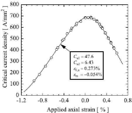
In figure 4[7] a typical current-strain curve is shown, in which this asymmetry is visible. “When a wire is subjected to uniaxial compressive strain, the critical current density, upper critical field and the critical temperature reduce approximately linearly and reversibly with strain. When a wire is subjected to a uniaxial tensile strain, the critical parameters increase approximately proportionally and reversibly with strain until a parabolic-like peak is reached, after which the properties reduce approximately linearly with strain”[20].

The maximum in the curve is reached when the deviatoric strain components in the A15 are minimized. This is not the same value as where the axial pre-compression is minimized, i.e. where

is counteracted.

The second model is the deviatoric strain model by Ten Haken [10]. This model incorporates the three-dimensional nature of the strain, but does not model the asymmetry around the maximum in the strain dependence curve (see figure 4).

The third model is the full invariant analysis proposed by Markiewicz [21]. This model uses a more microscopic approach and is therefore more complex, but also the best fit. The model does not yet incorporate a full description of the dependence of the upper critical magnetic field and the critical temperature on strain.

From here on the focus will lie on the proposed scaling law by Godeke. This scaling law fully describes the critical current density, , for uniaxial strains based on the deviatoric strain model. Here is the critical current density. Below the scaling law is shown:

11 (5) (6) (7) (8) (9) (10) (11) (12) (13)

The superconducting parameters , , and and the deformation related parameters , , and need to be determined experimentally. The parameters are listed in table 1

Parameter Description

Fitting parameter of the bulk pinning force ( )

Fitting parameter of the bulk pinning force ( )

_Constant

Maximum upper critical field at 0 Kelvin

Maximum Ginzberg-Landau parameter in strain dependence results

Inhomogeneity averaged critical temperature

Upper critical field

Inhomogeneity averaged maximum critical temperature in strain dependency results at

0 strain

Second invariant axial strain sensitivity Axial remaining strain term

Third invariant axial strain sensitivity Applied strain in axial direction

Axial pre-strain in the A15 phase

Table 1: Description of the parameters in the strain scaling law by Godeke.

Godeke used the deviatoric strain model as a starting point. From there he defined his model for uniaxial strain experiments. He added the linear term to the strain dependence, , to rotate

the curve around the maximum to account for the stronger reduction in critical current for tensile strains. Due to this the axial position of the maximum shifts by a factor . Also due to this the

maximum of increases above one and therefore is re-normalized to the

12

As stated before transverse pressure is documented in literature, but if scaling is regarded no qualitative scaling has been found to propose the incorporation of the influence of shear strains, besides the incorporation via the principal strains in the deviatoric strain or via the full invariant analysis. These methods have not been verified yet for a full three-dimensional analysis. So as with axial strain in the scaling law of Godeke, no scaling law exists in which current scales with the shear strain components. Also Ten Haken states that transverse strain experiments on have insufficient reproducibility to link them to the proposed deviatoric strain dependence of . Another

confusing finding was the decrease of with decreasing deviatoric strain in tapes. As from this, it

can be concluded that no applicable transverse strain dependence of the critical current has been formulated yet. It must be stated though that in wires a large reduction of the critical current has been observed in transverse strain experiments. This reduction has not been observed in tapes.

For the purpose of this thesis no scaling law has been found that describes the critical current as function of the full three-dimensional strain. The basis for such a scaling law is available in literature [7][4] [21], but these are not fully developed and have not been compared to a detailed mechanical study yet.

1.4

Parallel magnetic field

A Lorenz force exists when a magnetic field has an angle with a current. A normal electrical wire which is parallel to a magnetic field is therefore ‘force-free’. This is not the case for a parallel bronze route wire since the filaments are twisted and therefore, if the strand’s axis is parallel to the magnetic field, the filaments are not parallel to the field. From the paragraph above it is given that the critical current depends on the magnetic field strength. The ‘effective’ magnetic field strength increases with increasing angle between the strand’s axis and the magnetic field, reaching its maximum at . In figure 5 this is visualized[3].

Research about the critical current dependence on the magnetic field orientation is done by Schild [3] and Takayusa. Schild limits his research to the magnetic field orientation dependence due to manufacturing process. In chapter 4 a geometrical influence will be substituted.

Schild defines the reduced critical current as

(14)

Here is the angle of the strand’s axis with the magnetic field. A field strength dependence in noticed for high fields, above 15 Tesla, in the bronze route samples, but since the magnetic field strength in this thesis is small compared to the maximum upper critical field, this field strength dependance is not taken into account[3]. Therefore the magnetic field orientation dependence of the critical current is given by Takayasu’s experimental law

13

Where m and n are two fitting parameters and is the average angle of the filaments with the magnetic field. and are 0.83 and 0.19 respectively for a bronze route strand [3]. is given by

(16)

This is the integral over the filamentary cross section, taking into account that along the radius the filaments have a different angle with the magnetic field. is set as the angle that controls the critical current dependence of the magnetic field orientation [3]. is the filament distribution function and

is the angle of a filament with the magnetic field, given as

(17)

Here is the twist pitch.

1.5

Course of the assignment and lay-out of the thesis

In this thesis the influence of torsion on the critical current of is researched. Results are

obtained under parallel magnetic field for a bronze route strand. The scaling law of Godeke is used in combination with a 3D model from COMSOL and the orientation dependence by Schild, which results in a model for the critical current dependency on torsion.

The entire development of the experimental setup was done by R. Pompe van Meerdervoort. He also contributed the photos further on in the thesis. The experiments are done by R. Pompe van

Meerdervoort and myself. My contributions are also the development of the COMSOL model, the data processing and the alignment of the theoretical framework with the result.

14

2.

Modeling

2.1

Structure

From chapter one it is known that the strain state of the sample is important for critical current calculations. The purpose of this model is for it to be able to give good insight in the strain state within the A15 layer.

Within the Energy Materials and Systems group, COMSOL Multiphysics is often used for strand modeling. By choosing COMSOL as modeling program an easy understanding and adoption of the model within the group is possible.

After extensive effort to implement the thermo-mechanical modeling in combination with the mechanical modeling, the simplification has been made to model the pre-compressive strain ( ) directly.

Furthermore, a large part of the strand has been homogenized to limit the degrees of freedom in the FEM calculations. Since the only interest is in the strain state of the A15 layer, the copper, bronze and a large part of the filaments can be taken together in the homogenization. The model only has to simulate the induced strain in the filaments, which originates from the applied forces and the surrounding matrix material. The barrier material has not been accounted for.

Due to the expected radial differences in the strain when applying torsional deformation, a multifilament model has been made. Its structure can be seen in figure 6.

Figure 6: different views of the COMSOL model. Locations of the filaments from inside to outside, A to D.

The model has been built to the specifications in table 2. The filamentary area has been divided into four circular regions, each represented by one large filament. The height of this model is 1/8 of a twist pitch. This results in a strain state at the center cross section that should not have any influence of the entrance effects any more. This will be clarified later. The inner filament is placed just outside the strand’s z-axis and the outer filament just inside the filamentary area. From inside to outside we have filament A to D.

15

Bochvar strand parameter Value

Strand radius ( ) 0.405 mm

Filamentary area radius ( ) [28] 0.273

mm*

Twist pitch ( ) 15 mm

Number of filaments [23][29] 7225

Filament radius [23] 1.5 µm

Thermal pre-compression ( ) -0.110%**

Table 2: relevant specifications of the Bochvar strand investigated in this work.

*average of bronze route filamentary area radii

**from unpublished result of Pacman measurements on Bochvar strands

2.2

Calibration

Now the model needs to be calibrated to generate plausible outcomes of the strain state. Elastic properties are well documented in literature (elastic modulus and Poisson’s ratio). Also tensile strain experiments are well documented. The calibrations are done under the assumption of isotropic elastic properties for the geometry and subdomains.

Here two methods will be set forth to calibrate the model. The first uses an aerial approach, summing the volume fractions of the different materials with their elastic properties, to find the elastic properties of the homogenization. The second approach uses axial stress-strain results to determine the uniform elastic properties of the entire strand. From these the elastic properties of the homogenization are determined by subtracting the aerial fractional portion of the elastic properties of the four filaments.

First this was done for a model with 1 filament and a subdomain for the copper shell. Later the copper shell was integrated in the homogenization for simplicity. This simplification did not influence the calculated strain state of the A-15 phase. Also three more filaments were added, which also did not alter the strain state of the first filament. The strain state in the filament is calculated from the strain of the matrix on the filaments and the applied strain. The presence of the added filaments does not alter these strains.

In table 3 the values of the aerial homogenization are shown.

Material Volume fraction Elastic modulus Poisson’s ratio

Cupper 60 % 137 GPa 0.355

Bronze 26% 119 GPa 0.34

A-15 14% 100 GPa 0,39

Barrier 0 % 100 GPa 0.38

Homogenization 127 GPa 0.356

A-15 100 GPa 0.39

Table 3: Elastic properties of strand materials [23, 29-32] and the homogenized elastic properties by using an aerial approach.

16

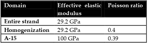
range between 70 MPa and 156 MPa stress, in other words between 0.0012 and 0.004 strain. By extrapolating this curve down as if the stress-strain curve of the Bochvar stand is linear, an extra term to the intrinsic strain is added. The Poisson’s ratio of the homogenisation is estimated at 0.4. The added offset in the pre-compressive strain is -0.001. The elastic properties are shown in table 4.

Domain Effective elastic

modulus

Poisson ratio

Entire strand 29.2 GPa

Homogenization 29.2 GPa 0.4

A-15 100 GPa 0.39

Table 4: elastic properties for the modeling of the Bochvar strand in COMSOL by using the stress-strain curve and the ‘effective elastic modulus’.

Figure 7: Measured stress-strain curve for a Bochvar strand by the EMS group at Twente University.

It would be expected that both approaches would deliver the same result, since both give a good approximation of the reality. Intuitively it can be stated that this is not the case, since the elastic moduli of the homogenizations differ by a factor of four. Therefore the second calibration will be used for the remainder of this thesis, because this calibration gives a much more reliable output for axial strain modeling in the domain of interest. Note that this is only a good approximation as long as the stress (or strain) increases (figure 7). The difference in the value of the elastic modulus and the effective elastic modulus can be assigned to plastic deformations in the matrix material and copper [26]. In the stress-strain curve it can also be seen that the strand deforms plastically in the low strain regime (0 to 0,002), so it might be possible that the slope of the curve at zero strain is ~127 GPa. This is then also the case for all points along the x-axis where the stress increases from zero.

17

zero when a force on the top boundary is applied. This force should result in 0.0011 axial strain on the strand, hence, the strain in the filaments in the z-direction should be 0. As can be seen in table 5 (and figure 7) this force should be 65 MPa. On the x-axis the length of the simulated filament is shown as function of length of a twist pitch in radians. The simulated twist pitch is ¼ of one total twist pitch (2π).

Figure 8: Strains in the strand for different stresses. Figure 9: Strain in the filaments at 65 MPa axial stress.

Applied stress Strain strand from literature

Strain strand from model

Error

65 MPa 0.0011 0.00105 5%

95 MPa 0.002 0.00203 2%

125 MPa 0.003 0.00305 2%

156 MPa 0.004 0.00403 1%

Table 5: Comparison of the literature with the output from the COMSOL model.

2.3

Results and discussion

The modeling in COMSOL has been done under de assumption of a homogeneous distribution of twist and axial strain within the sample.

As explained in paragraph 2.1 torque is applied on the top edge of the model. Some results of the uniaxial strain (z-component strain) can be seen in figure 10.

18

Figure 10: strains at two angles of twist for the 1/8 Figure 11: strains at two angles of twist for the 1/4 twist pitch length model. twist pitch length model.

Twist Filament Value model 1 Value model 2

180 A 0.00018 0.00018

B 0.00022 0.00022

C 0.00029 0.00029

D 0.00038 0.00038

720 A 0.00019 0.00019

B 0.00034 0.00034

C 0.00065 0.00065

D 0.00108 0.00108

Table 6: Comparison of the strains in model 1 (1/8 twist pitch length) and model 2 (1/4 twist pitch length

For a transverse strain calibration better results should be available on bending strain on bronze route strands. In [17] and [16] are modeling and measuring methods of transverse pressure proposed. So a better calibrated model can be obtained by implementing thermo-mechanical aspects and improved material properties. Also the plastic properties of the strand should be modeled in that case [17]. For now the axial calibration gives a good sense of the ligidity of the results. The transverse calibration is out of the scope of this thesis.

This model is used throughout this thesis, but a check on some parameters in a later stage gave some results regarding the deviatoric strain. From literature it is known that at an axial strain close to the axial pre-compression the deviatoric strain minimizes [10]. This is at a strain δ. For the strand in the thesis this value is unknown. In figure 12 the deviatoric strain is plotted against the axial tension. At 62.5 MPa the deviatoric strain minimizes. This is close to the value of the axial pre-compression, but since no value for δ is known, no conclusions can be drawn regarding the precision of the model if it comes to the deviatoric strain.

19

Another comment on the model is the value for the Poisson’s ratio (0.4), which is not a logical choice if compared to the result of the Poisson’s ratio from the homogenization (0.356). Due to time constraints the calculation for the entire model are not redone, but one value is obtained for an angle of twist (ϕ) of 720° with a Poisson’s ration of 0.356. The value of the deviatoric strain changed by 2% where the Poisson’s ratio changed by 11%.

2.4

Conclusions

20

3.

Experimental details

3.1

Configuration and setup

The experiment is done in the 15 Tesla cryostat at the EMS group of the University of Twente. This device has a boring diameter of 80 mm.

The cryostat maintains a constant temperature of 4.2 K during operations.

An external field is applied on the sample during operations by an electromagnet inside the cryostat. The field is assumed perfectly parallel to the sample axis. Deflections from the center of the cryostat will be present, but are intuitively ignored because these are very small and the magnetic field strength does not change substantially in that region. In figure 13 is visible that the magnetic field will not have the same field strength along the entire length of the sample, which is 157 mm. The center of the sample is located at the center of the cryostat. From figure 13 it can be estimated that the magnetic field strength decreases about 9% from the center to the edge of the strand, namely 1.8 Tesla decrease over 10 cm when the center has a field strength of 15.6 T.

Figure 13: Magnetic field strength in the 15T cryostat at the EMS group. Picture by Jeroen van Nugteren.

For the experimental research an adapted version of the TARSIS insert was used. Modifications have been made to freeze all degrees of freedom, except two. The part of the insert at cryogenic temperatures can be seen in figure 14.

21

Figure 14: Insert at strand level with the strand inside (left) and the strand’s fixation (right).

Secondly the angle of twist is a degree of freedom, which also is applied from outside the cryostat on the central shaft to the top cylinder.

The central copper shaft was also used as current lead. Current passes through shaft and the top copper cylinder into the strand, into the lower cylinder, into two YBCO tapes and into the bottom copper parts. The YBCO tapes are soldered at the ends to the copper block on the bottom and are free to move at their centers. This structure makes sure that the bottom copper cylinder is still ‘free’ to move to account for the shrinking of the setup. The setup is able to deliver currents of more than 750 Ampere to the strand.

The bottom copper cylinder fits into a G-10 holder (see figure 14), which holds it in place and acts as a clamp for the cylinder to go up, when pulled up during testing. Later this axial load will be further clarified.

The strand is supported along its length by the G-10 holder and a reinforced ceramic tube (see figure 14). The ceramic tube is being held in place by G-10 struts. This way the Lorenz forces will not affect the position of the strand.

Most materials used in the setup do not magnetize. If so, the materials surrounding the sample would influence the angle and strength of the externally applied field, and therefore the measurements. Magnetization does occur in the copper parts. The effect of this magnetization is neglected in this thesis because the distortion of the field is very small compared to the applied field and no copper parts are ‘near’ the sample (further away than a few µm), this means the sample will not ‘feel’ the presence of the copper parts in the setup.

22

voltage pairs), the magnetic field and the applied axial force. For the applied axial force a voltage is measured from which the actual force in Newton can be calculated.

Each device has an error. Later a decision has to be made if these errors are of significance or not. Below you will find an overview of the devices, the specifications and the errors in the measured parameter. The errors originate from the datasheets of the devices and are an approximation of the total error in the measured parameter.

Device Measured parameter Error Range and notes

Hitec Zero-flux Current (A) Max. 0.9 A Type B2000

Range: 200 to 750 A

Keithley Model 1801 Nanovolt Preamp with 2001

Voltage (V) 0.3 nV Range: 1 to 10 µV

Keithley 2182A

Nanovoltmeter

Voltage (V) 40 nV Range: 1 to 10 µV

Cryogenic magnetic

power supply

CTS-91/25

Magnetic field (T) ~10 mT Type PS120C Range: 14 T

Tedea Huntleigh model 615 with Keitley 2000 multimeter (loadcell)

Voltage (V) 3 µV Range: 0.25 mV

Table 7: List of experimental devices used in the experiment and their final error in the measured parameter.

It is expected that these errors do not have a significant influence on the experimental results, since they are all, at least, a hundred times smaller than the measured parameter. Most are in the range of a thousand times smaller than the measured parameter.

Furthermore, VI was used to process the data. It calculates the V-I graphs, the critical currents and n-values of the experiment.

3.2

Materials and Methods

Due to the extremely brittle A15 phase in the sample, the sample had to be handled very carefully. Another important step of the sample preparation is good electrical contact with the current supply. Only the most important steps of the sample preparation will be reported here.

When the sample was soldered into the cylinders and the cylinders were placed into the setup, good electrical contact was guaranteed by etching away the outer chrome layer of the strand, and by scrubbing down the copper layers of the cylinders and the inside of the central shaft.

A G-10 sample holder was used to prevent the strand from breaking, see figure 15. This holder was also used to place the sample in the insert. When placed in the setup the voltage taps were soldered on. 5 voltage pairs were used to measure the voltage over the strand at different positions. The lengths can be seen in table 8. The length of a section is used to calculate the electrical field strength, which is a measure for the resistance as described in paragraph 2.1. The wires used for the voltage pairs do not lay any restrictions on the movement of the strand.

23 Figure 15: Sample holder

The torsion experiments are the first to be executed on wires. This experiment is the first experiment with a combination of axial strain, torsional strain and parallel magnetic field.

Various attempts have been done with this setup on internal tin wires, without proper results. From these experiments it can be concluded that high magnetic field strengths, of 14 Tesla, are needed to measure a critical current. Therefore the experiment is conducted at 14 Tesla, parallel field. Also, caution is required regarding the current supply. Too much current can lead to a quench in the strand, and in its turn this can lead to a temperature of the strand higher than the melting point of the soldering used to attach the voltage pairs, i.e. the voltage pairs will come loose.

As explained in chapter one, within a certain range it is said a material is superconducting. This range is specified by the critical field, defined as 10 µV/m. During measurements the current increases and the voltage (or electrical field) of the different voltage pairs is measured. This results in V-I curves shown in figure 18. VI calculates the associated critical current by extrapolating down to the field criterion from the measured values in the range of 100µV/m to 1000µV/m. The VI settings are given in table 9.

It is assumed that at the start of the experiment the sample has not experienced plastic deformations from, for instance, sample handling and shrinkage. To freeze out the degrees of freedom at the bottom of the sample a uniaxial force was applied, by the loadcell, to pull the strand in tension. This locks the bottom copper cylinder in the G10 holder, see figure 14. When the sample is unloaded, a voltage of 0.1 mV was measured by the load cell. A stress of 70e6 N/m² is applied to the strand, which corresponds to a voltage of 0.25 mV. It is assumed that the applied load at the top of the insert is the load applied on the strand. This axial load also result in a critical current to the right of the maximum critical current, see figure 4.

Voltage pair Location Length

1 Top 23 mm

2 21 mm

3 Center 30 mm

4 22 mm

5 Bottom 23 mm

Table 8: Voltage pair locations and lengths.

Setting Value

Critical field criterion (V/m) 1e-5

Current margin (A) 3

Margin upper critical field (-) 100 x critical field

Margin bottom critical field (-) 10 x critical field

Table 9: VI-settings for critical current calculations

24

Because of the temperature gradient during an experiment, the materials in the setup expand. This would result in a smaller uniaxial force if not compensated for. Therefore the uniaxial load was maintained at 0.25 mV.

25

4.

Results & discussion

In this paragraph the results from the experiment will be presented and discussed. Then two different effects of torsion, namely the geometric and mechanical effect, will be further examined in search of an explanation for the experimental result.

The experimental result was obtained from a Bochvar strand, which is a bronze route strand. The measured critical current of the different sections is plotted against the angle of twist in degrees in figure 17. The electrical field of section A and E was too low to calculate a critical current until an angle of twist of 840 degrees. The same is the case for sections A and D until an angle of twist of 180 degrees. The result shows good symmetry along the strand’s length. This suggests a homogeneous distribution of force and twist, that is also assumed in COMSOL. A critical current for section C was calculated for the first time at an angle of twist of 120 degrees. Lower angles of twist did not result in a strong enough electrical field to calculate a critical current. Note the supplied current did not exceed 750 A. The reason for this was a lack of insight in when the strand would quench as stated in paragraph 3.2.. The curve at 120 degrees suggests a flattening of the slope for lower angles of twist. In axial strain experiments the critical current of the strand without twist is in the parabolic region for an axial load of 70 MPa. This would also suggest a decreasing slope with increasing angle (see figure 4). Other torsion experiments need to be conducted to confirm this suspicion of the lower torsional region.

Figure 17: Critical current plotted against applied angle of twist on a bronze route Bochvar strand under 14 Tesla parallel magnetic field. Ic A is the top voltage pair and Ic E is the bottom voltage pair.

Figure 18 shows the V-I curves at an angle of twist of 840 degrees made in VI. From this figure the following can be concluded:

26

Earlier it was explained that the magnetic field declines about 9% along the strand’s length from center to edge. A decline in electrical field results in a higher critical current. Is differentiation in the critical currents along the sample length a result of a different applied magnetic field? Literature states it is, since a lower magnetic field in the parralel direction means a lower effective magnetic field and thus a lower Lorentz force, i.e. a higher critical current.

Figure 18 also suggests that the wire is homegeniously twisted, since the two outer voltage pairs (curve 1 and 5) are relalitively close to eachother and have comparible slopes. The same is the case for the voltage pairs next to the center voltage pair (curve 2 and 4).

Figure 18: V-I curves at 720 degrees twist. 1=top voltage pair to 5=bottom voltage pair.

Looking at the result in figure17, a distinction is made between different influences on the result. First of all it is expected that due to torsion the field orientation changes. The filaments inside the strand are not parallel to the magnetic field and therefore not in the force-free state. The filaments are twisted and make an angle with the field. When right-handed torsion is applied, which is the case, the twist pitch of the filaments decreases and the angle with the magnetic field increases, resulting in a larger effective field and thus a decrease of critical current with increasing angle of twist.

T. Schild suggested formulas to calculate the magnetic field orientation dependence of the critical current of , as can be seen in paragraph 1.4. Rewriting these formulas to fit the purpose of this thesis, i.e. the influence of torsion and parallel magnetic field, gives the following formula.

(18)

Originally was , because the twist pitch was constant. The angle between the magnetic field and the strand’s axis is known and the twist pitch is written as

27

L is the sample length and is the twist pitch without deformations. To plot the critical current against the angle of twist we take Ic(90°,0) as the critical current of an unloaded Bochvar strand in transverse, 14 Tesla, magnetic field. Also, to avoid time consuming calculations, was calculated for the experimental values of . The resultant plot of the critical current’s geometrical effect is shown in figure 19.

Figure 19: Geometrical effect of torsion on the critical current. The experimental average and the model of T. Schild plotted against the applied angle of twist.

The resultant curve shows a small dependence on the changing angle with the critical field due to torsion. The critical current is inversely proportional with the angle of twist, as expected. The small impact of the geometric effect on the critical current is intuitively explained by little changes in twist pitch do to torque. These small changes in twist pitch are visible almost one-to-one in the critical current since the sinus of a small angle (formula 18) is in approximation that small angle. It can be concluded that the geometrical effect of torsion does not ‘control’ the critical current.

28

Figure 20: Mechanical effect of torsion on the critical current by using the z-component of the strain from COMSOL. The experimental average and the scaling law of Godeke plotted against the applied angle of twist.

The slope of de scaling law is slightly negative. From this it can be concluded that the axial component of the strain is not the ‘controlling’ strain component of the critical current in the case of torsional deformation, so the scaling law of Godeke is not suitable for critical current calculations in this case. This is not surprising since in uniaxial experiments the transverse components of the strain have little influence [10] and therefore these components are not taken into account in the scaling law of Godeke. The scaling law by Godeke is based on a combination of the invariant analysis and the deviatoric strain model. From here on two different approaches will be evaluated to find the strain that controls the critical current. Godeke uses the uniaxial strain ( ) and an orthogonal coordinate system in which the principal strain direction are the same as the coordinate system axles. Then, from literature, the deviatoric strain is defined as:

₍₁₉₎

From the discussion above it is now known that the simplification from to is

not applicable to torsional deformations. The two alternatives are:

1) The critical current is determined by an orthogonal coordinate system, which also includes ‘off axial’ components of the strain, namely and . This also means the off axial components are not linearly related to the applied uniaxial strain by Poisson’s ratio, as done by Ten Haken and Godeke. Since in an orthogonal system , and , the off axial components and the uniaxial component from the COMSOL model should be inserted in the deviatoric strain.

29

Both alternatives are not described in literature. The scaling law in literature uses uniaxial strain and the constants in the scaling law are determined by experiments, as described in [20]. Therefore the insertion of the deviatoric strain in this scaling law will not be scaled properly, i.e. the superconducting and deformation related parameters do not have the correct value. Godeke relates to uniaxial strain to the off axis strains by the Poisson’s ratio, as can be seen in formula (20). If now the deviatoric strain is determined from the principal strain tensor, the value of the deviatoric strain is in close approximation with the applied axial strain. This is shown in formula (21).

₍₂₀₎

₍₂₁₎

is the principal strain tensor.

Though the use of the scaling law, in combination with the two alternatives, is not correct, the argument above suggests that the use of the deviatoric strain will be a good enough approximation, mainly, to get an idea of the influence of the two alternatives on the critical current, i.e. the scaling law will allow the use of the deviatoric strain without large errors.

Note that the change of the principal coordinate directions in alternative 2 does not change the formula of the deviatoric strain, since the deviatoric strain is an invariant of the deviatoric strain tensor and thus independent of the coordinate system.

From COMSOL the uniaxial strain (z), the y- and x-component of the strain and the principal strains, all at different angles of twist and in the different filaments are known. Each filament in the COMSOL model represents a part of the cross section of the strand. A fractional aerial summation has been done to get a strain value that describes the average strain in the strand. These have been substituted in the scaling law. The critical current, as result of the strain, at different angles of twist, is then calculated. These critical currents are substituted for in Schild’s formula. The resultant curve is the model of the critical current as function of the angle of twist, that combines the geometrical and mechanical effect for uniaxial strain, orthogonal strains and principal strains. The result is shown in figure 21.

30

Figure 21: Geometrical and mechanical effect of torsion combined by using the z-component of the strain, the orthogonal components of the strain and the principal strains in the scaling law. Also the experimental average has been plotted.

Three main errors can be pointed out. First of all, the scaling was done for a uniaxial modeling. The influence of this error is expected to be minimal, since the unknown parameters of the scaling law only twist it around the critical current’s maximum to account for the difference in strain sensitivity for compression and stretching. This change in slope (sensitivity) is also suggested by the experimental result. The linear curve from the orthogonal model can therefore not be reshaped to the experimental results by rescaling.

Another influence in the error can easily be seen from figure 22. The shear strains are plotted on the y-axis for filament D. From figure 22 it can be seen that the XZ and YZ shear strains are not close to 0 and increase with increasing angle of twist. These are the cross-sectional shear strains and when plotted against an entire twist length should give a sinusoidal curve [33]. The orthogonal model does not account for these shear strains.

31

Figure 22: Shear components of the strain inside filament D for 180 and 720 degrees of twist.

Now the principal strain approach is discussed. It is discussed that the influence of shear strains should be accounted for. Therefore a method that takes into account the three dimensional character of torsional deformation has to be used. The deviatoric strain does account for this if the ‘true’ principal strains are used, i.e. not just the orthogonal strains. Figure 21 shows reasonable agreement with the experimental result in the low twist region (up to 360° angle of twist). In the high twist region the influence of strain is overestimated. Now the expected causes are discussed.

The modelled graph is not linear over the entire twist region, which confirms the suspicion of a flattening slope towards the zero twist point. Therefore the scaling is important for improved results. As stated before, the constants in the scaling law rotate and shift the result and determine the sensitivity of the critical current to strain. Determining the parameters in the scaling law can result in a better corresponding output. Estimated form the modelled curve, the counter clockwise rotation around the maximum critical current should be larger, and/or the sensitivity to compressive shear strain and axial strain should be lower, i.e. should be lower (less rotation). Also, should be

and account for the non-axial, remaining strain components when the axial strain is zero.

As stated by Godeke: “the performance of this model is assessed by determining how well the model fits data from uniaxial strain experiments. However, it remains to be seen how well the model performs with the direct use of the three-dimensional form in a detailed mechanical analysis”[4]. The same conclusion is draw above.

32

A better evaluation of the principal strain model can be made by generating more data points and comparing these with the experimental result.

Resultant from the above discussion is that the principal strain approach should be applied to model the effect of torsional deformations on the critical current. This because it takes into account the shear components of strain, which cannot be neglected when a strand is twisted.

Briefly a few other effects and results will be pointed out.

Since the magnetic field makes small angles with the filament axles, the question arose if the self field has an influence on the angle of the magnetic field with the strand axis ( ). The self field’s maximum is 0.37 Tesla at 750 Ampere. The angle of the resultant field, with regard to the sample’s axis, will not be zero degrees, since a helical field will be present due to the self field. The deflection of the parallel field due to the self field will be 1.5 degrees for a current of 750 Ampere. Since the filaments make an angle with the magnetic field of the same order of magnitude, i.e. in the order of 5°, the influence of the self field for parallel field experiments should be examined.

33

5.

Conclusion

5.1

Main conclusions

The first experimental results are obtained on bronze route , on which torsional deformations have been applied. These results are obtained in parallel magnetic field. Several models have been proposed to calculate the critical current via the scaling law of Godeke. The output of the scaling law was scaled via Schild’s formula to model the parallel magnetic field. It was found that the geometrical effect of torsion, i.e. decrease in twist pitch, does not have a significant influence on the critical current. It has been determined that the deviatoric strain, which uses the principal strains, is the strain that determines the critical current dependency on torsional deformation in parallel field. This is due to the increase of the cross sectional shear strain components with angle of twist. This increase cannot be neglected. The scaling law used in this thesis does not suffice, due to its uniaxial nature. From the experimental results and the modeling it is suspected that the slope flattens for lower angles of twist and under this suspicion it can be stated that the critical current does not degrade for practical angles of twist.

5.2

Recommendations

Regarding the COMSOL model several recommendations can be made. The linear homogenization made in paragraph 2.2 leads to a limited applicability. To increase this, first the plastic deformation of the matrix and the copper need to be implemented as suggested by T. Wang [17]. Also the implementation of the thermo-mechanical aspect, due to the cool down to cryogenic temperatures, gives a more realistic reproduction of the real strand. Finally the model should be calibrated for torque and bending. The calibration with torque can be easily established by measuring the force needed to apply a certain angle of twist. Due to this it might be necessary to incorporate the anisotropic strain dependence of a strand. The calibration of bending is of less importance. Comparing the model with bending experiments will lead to a better understanding of the applicability of the model in torsional experiments, since torsion is a combination of applying radial shear strain and axial strain. It will result in a better understanding of the anisotropy.

It is also recommended to expand the strain scaling law so that it can cope with the three-dimensional nature of strain. Therefore systematic experimental research needs to be done on the critical current dependency on three-dimensional strains. The basis for this scaling law is proposed by [4]. Relations need to be found that describe the upper magnetic field and the critical temperature dependence on the strain (or rather the strain invariants). The full invariant analysis can also be used to describe the critical current accurately, but its complexity and many parameters make in less favorable for practical applications.

34

The increase of the n-values must be further research by looking at crack formation due to torsional deformation. Also, the experiments should be repeated in a more homogeneous magnetic field so that there is no change in the magnetic field strength along the strand’s axis.

In appendix B the experimental result shows a single data point at 360°. This result is obtained by returning the angle of twist form 1080° to 360°. The critical current shows little reversibility. Further research should be done to determine the degree of reversibility of the critical current.

35

6.

References

1. Soren Prestemon, Paolo Ferracin, Ezio Todesco.Basics of superconductivity. s.l. : U.S. Particle

Accelerator School, June 2007. 2. www.wikipedia.nl. [Online]

3. T. Schild, H. Cloez. Magnetic field orientation dependence of critical current in industrial Nb3Sn

strands. Cryogenics. 38, 1998, pp. 1251 - 1257.

4. An improved model for the strain dependence of the superconducting properties of Nb3Sn. Arbelaez, D.,

Godeke, A., Prestemon, S. Berkeley : Superconductor Science and Technology, 2009, Vol. 22.

5. B. ten Haken, A. Godeke, H.H.J. ten Kate. The strain dependence of the critical properties of Nb3Sn

conductors. Applied Physics. 6, 1999, Vol. 85.

6. A Review of the Properties of Nb3Sn and Their Varioation with A15 Composition, Morphology and Strain State. Godeke, A. Berkeley : Superconductor Science and Technology, 2008.

7. Godeke, A.Performance Boundaries in Nb3Sn Superconductors. Enschede : PrintPartners Ipskamp,

2005. ISBN 90-365-2224-2.

8. The deviatoric strain description of the critical properties of Nb3Sn conductors. Godeke, A., Ten Haken,

B., Ten Kate, H. Enschede : Physica C, 202, pp. 1295 - 1298.

9. Strain Dependence of Critical CUrren in Internal Tin Process Nb3Sn Strands. Sangjun Oh, Soo Hyeon

Park, Chulhee Lee, Yongbok Chang, Keeman Kim and Pyeong-Yeol Park. 2, s.l. : IEEE Transactions

on applied superconductivity, 2005, Vol. 15.

10. Ten Haken, B.Strain effect on the critical properties of high-field superconductors. Enschede :

Universiteits Drukkerij Enschede, 1994. ISBN 90-9007519-4.

11. The influence of Compressive and Tensile Axial Strain ont the Critical Properties of Nb3Sn Conductors.

Ten Haken, B., Godeke, A., Ten Kate, H. 2, Enschede : IEEE Transactions on applied

superconductivity, 1995, Vol. 5.

12. The strain dependence of the critical properties of Nb3Sn conductors. Ten Haken, B., Godeke, A., Ten

Kate, H. 6, Enschede : Applied Physics, 1999, Vol. 85. 0021-8979/99/85(6)/3247/7.

13. A Novel "Test Arrangement for Strain Influence on Strands" (TARSIS): Mechanical and Electrical Testing of ITER Nb3SN Strands. Wessel, W., Nijhuis, A., Ilyin, Yu., Abbas, W., Ten Haken, B. et al. Enschede : Advances in Cryogenic Engineering, 2004.

14. Effect of transverse compressive stress on the critical current and upper critical field of Nb3Sn. Ekin, J.W.

4829, Boulder : Applied Physics, 1987, Vol. 62.

15. The influence of Nb3Sn strand geometry on filament breakage under bend strain as revealed by

36

16. Axial and transverse stress-strain characterization of the EU dipole high current density Nb3Sn strand.

Nijhuis, A., Ilyin, Y., Abbas, W. 065001, Enschede : Superconductor Science and Technology, 2008,

Vol. 21.

17. Fundamental simulations of transeverse load effects on Nb3Sn strands using finite element analysis. Wang,

T., Chiesa, L., Takayasi, M. Cambridge : Advances in Cryogenic Engineering, 2012.

18. David M J Taylor, Damian P Hampshire. The scaling law for the strain dependence of the critical

current density in Nb3Sn superconducting wires. Supercond. SCi. Technol. November 4, 2005, pp. S241-S252.

19. Strain scaling law for flux pinning in practical superconductors. Part 1: Basic relationshop and application to Nb3Sn conductors. Ekin, J.W. s.l. : Cryogenics, 1980. 0011-2275/80/011611-14.

20. A general scaling relation for the critical current density in Nb3Sn. Godeke, A., Ten Haken, B., Ten

Kate, H. and Larbalestier, D. Enschede : Superconductor Science and Technology, 2006, Vol. 19.

21. Markiewicz, W. Denis. Invariant temperature and field strain functions for Nb3Sn composite

conductors. Cryogenics. 46, 2006.

22. Lectures on applications of superconductivity 1 & 2. Kate, Ten. Enschede : s.n.

23. Recent progress of low temperature superconducting materials at Bochvar Institute. Potanina, L., Shikov,

A., Vedernikov, G. et al. 386, Moscow : Physica C, 2003, pp. 390 - 393.

24. A thermo-mechanical model for Nb3Sn filaments and wires: strain field for different strand layouts. Boso,

D., Lefik, M. Padua : Superconducto Science and Technology, 2009, Vol. 22.

25. Fabrication and characterization of internal Sn and bronze-processed Nb3Sn strands for ITER application.

Zhang, P., Li, F., Liu, J. Li, C., Zhang, K. et al. Xi'an : Superconductor Science and Technology, 2010,

Vol. 23.

26. Axial tensile stress-strain characterization of ITER model coil type Nb3Sn strands in TARSIS. Van den

Eijnden, N., Nijhuis, A., Ilyin, Y., Wessel, W., Ten Kate, H. Enschede : Superconductor Science and

Technology, 2005, Vol. 18.

27. Eunguk Lee, M.S.AC Loss in superconducting composites: continuous and discrete models for round and

rectangular cross sections, and comparisons to experiments. Ohio : s.n., 2004.

28. Sanabria, C. Measuring the average radius of Fillamentary Area Radius for the ITER strands. s.l. :

Applied Superconductivity Center, National High Magnetic Field Laboratory.

29. Shikov, A., Pantsyrny, V., Vorobieva, A.,Vedernikov, G. Investigation on technical

superconductors for large magnet systems in Bochvar Institute. s.l. : Bochvar Institute of Inorganic Materials, 2004.

37

31. Nyilas, A., Weiss, K. Biaxial strain response of structural materials and superconducting Nb3Sn

wires at 295 K, 7K and 4K. Advanced cryogenic engineering. 2008, Vol. 54. 32. http://www.engineeringtoolbox.com/. [Online]

33. Theoretical Modeling for the Effect of Twisting on the Properties of Multifilamentary Nb3Sn Superconducting Strand. Jing, Z., Yong, H., Zhou, Y. 1, s.l. : IEEE Transactions on applied superconductivity, 2013, Vol. 23.

34. Ekin, J.W. Strain scaling law for flux pinning in practical superconductors. Part 1: basic

relationship and application to Nb3Sn conductors. Cryogenics. November 1980.

35. Transverse load optimization in Nb3Sn CICC design; influence of cabling, void fraction an strand stiffness.

38

7.

Appendices

Appendix A

In the last indention of chapter 4 some remarks are made about the n-value data. Below this data can be found. Figure 23 and 24 show data from VI. Figure 23 shows the electrical field plotted against the current for all the voltage pairs at 60 degrees of twist. Here significant electric field can be noticed. Also a steady rise of the curves with a n-value above one is noted.

Figure 23: V-I curves at 60 degrees twist. 1=top voltage tap to 5=bottom voltage tap

Figure 24 shows the electrical field plotted against the current for the centre voltage pair at all the angles of twist. The upwards shift of the ‘feet’ of the curve, indentified in the last indention of chapter 4, is clearly visible if curve 1 and 18 are compared. In table 10 the legend shows which number represents which angle of twist.

39

Number of the curve

Angle of twist

(°)

1 0

3 60

4 120

6 180

8 210

9 270

11 330

12 360

13 420

14 480

16 540

18 600

19 720

20 840

Table 10: Angle of twist per curve shown in figure 24

Figure 25 shows the n-values obtained from the experiment plotted against the angle of twist for all the voltage pairs.

40

Appendix B

In the final indention of paragraph 5.2 a remark is made about the reversibility of the deformations. A single data point is obtained after returning the angle of twist to 360 degrees from 1080 degrees. This is shown in figure 26 and gives an indication of the reversibility of the critical current.

Figure 26: Torsion on a bronze route Nb3Sn strand with reversibility data point. The sample is twisted back to 360 degrees from 1080 degrees

Appendix C

From COMSOL different strain values were obtained to be implemented in the scaling law of Godeke. These strain values are plotted against the angle of twist in figure 27. In future research it might be preferable to make a comparison between strain models and the one used it this thesis.