Saturation for LTSmin

(1)

Saturation for LTSmin

Master Thesis

Final project (course code 192199978)

Course year 2011 – 2012

Tien Loong Siaw (s0045217)

Master Computer Science

Track Software Engineering

Graduation committee:

■

prof. dr. J.C. van de Pol

■

dr. J. Ketema

■

prof. dr. ir. A. Rensink

Department of Formal Methods and Tools (FMT)

University of Twente

(2)

(3)

3

Abstract

State space generation or reachability analysis plays an important role in model checking, but a disadvantage of current techniques lies in the fact that they require quite a lot of time and memory to come up with a result when using real-life system models. Symbolic state space generation using known traversal techniques as breadth-first search and chaining are quite common practice, but their

performance on real-life system models with a large transition relation remains an issue to be tackled. In the past decade a relatively new traversal technique has emerged, named Saturation. This traversal technique has proven itself to be a good competitor to traditional symbolic state space generation

techniques for handling models with extremely large state spaces. It originates from the research group of professor Gianfranco Ciardo (University of California at Riverside, USA).

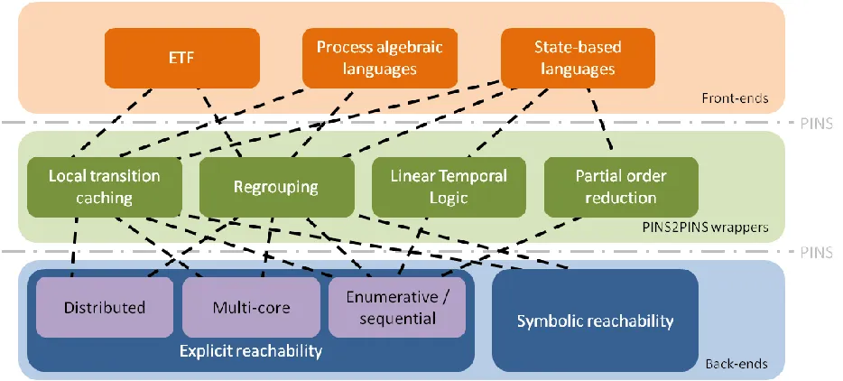
The main goal of this Master project is to design and implement the aforementioned Saturation-based approach in the LTSmin toolset, which is a set of verification tools developed by the Formal Methods and Tools group (FMT) at the University of Twente. The main features of this toolset is its setup in

architectural layers to separate language-specific details from verification algorithms and the use of an interface for presenting the (partitioned) transition relation of the model, called PINS.

The goal includes making adjustments to the LTSmin architecture for Saturation to work properly and comparing the implemented Saturation algorithm with other available symbolic reachability techniques in the LTSmin toolset.

An analysis of the Saturation-based approaches by G. Ciardo and the architecture of the LTSmin toolset is performed to choose the Saturation approach which fits best into the LTSmin toolset. The chosen (stand-alone) Saturation algorithm is then adjusted for implementation. The first version of this adjusted algorithm takes a different approach when updating the partitioned transition relation of the model compared to the algorithm proposed by G. Ciardo and reuses available functionality from the LTSmin toolset. An evaluation of this first version of the Saturation algorithm is performed comparing it to the other available reachability methods breadth-first search, chaining and an LTSmin version of a Saturation-like approach.

The evaluation reveals that the update process of the partitioned transition relation does not perform well for complex models resulting in bad time performance. Therefore the update process of the partitioned transition relation is revised. Hereby inspiration is taken from the update process used by G. Ciardo. This has resulted in a Saturation algorithm that outperforms the previous version of this

Saturation algorithm and comes out on top of the traditional traversal techniques breadth-first search and chaining with regard to time performance. Compared to the LTSmin version of a Saturation-like algorithm it performs competitively well too.

(4)

(5)

5

Preface

Initially I began my life as a student at the University of Twente in the autumn of 2002 by studying Industrial Design, but after fours years I realised this is not what I wanted to continue later in my career. So a year after I obtained my Bachelor degree in Industrial Design (in the autumn of 2005) I took the decision to switch over to Computer Science (in the autumn of 2006) where I hoped to find the career path that I was looking for. My interests in the field of Computer Science were initially in software design and especially in providing the graphical user interface of a software program. In numerous study projects and assignments throughout the years I was mainly responsible for the creative and user-oriented side of the project. Being creative and creating things was and still is one of the things I cherish in my life. In the last few years of studying Computer Science I discovered other interests in this field, namely software verification and algorithmic design challenges. The latter is due to a number of individual projects that I performed, such as designing and implementing an algorithm to detect rip currents in images of a shoreline (as part of the minor at the ITC in the winter of 2009), displaying UML diagrams more user-friendly on a screen (in my traineeship at Novulo in the second half of 2010) and adapting the Saturation algorithm as new state space generation technique for the LTSmin toolset, which is the subject of my graduation project.

In all these individual projects concerning an algorithmic design and implementation, I was initially quite hesitant about the assignments themselves, because the descriptions of the assignments were very technical and it is hard to imagine what challenges you have to face. But in all these cases it turned out that my initial hesitation was unnecessary. It was interesting to work on such challenging projects, together with the good support that was provided by my supervisors.

For my graduation project I came into contact with Jaco van de Pol at the end of 2010 and he suggested me to work on the Saturation algorithm as state space generation technique. Since then I worked on this subject for a year now which started with a better understanding in the new technique in Research Topics, followed by the graduation project in July 2011. Next to my main supervisor Jaco van de Pol, my weekly supervisor used to be Michael Weber. He was of great assistance when I faced difficulties, but nearing the end of Research Topics I noticed that Michael was busy preparing himself moving to the USA. After his departure and the completion of Research Topics, I was assigned a new weekly supervisor, namely Jeroen Ketema. With him as supervisor, I had regular weekly meetings to discuss my progress and to provide me with useful feedback. Although there were times he could get agitated slightly for my lack of clarity in some of my e-mail correspondences with him, he also helped me out at times when I was stuck when working with the LTSmin toolset. Next to the weekly meetings with Jeroen, I also had monthly meetings with both Jeroen and Jaco, which mainly focused on my progress. With their guidance and feedback I can finally present to you this report.

After studying for almost ten years at the University of Twente, my life as student comes to an end. First of all I want to thank my supervisors Jaco and Jeroen for their guidance, structural feedback and good response on my work. Secondly I would also like to thank Michael for being my initial supervisor on this subject and for his help on my initial work. Furthermore I would also like to thank my study advisor for supporting me throughout the years and give a helping hand from time to time. My final thanks go to my friends and family, especially my parents for having the patience to let me finish my studies. Although they did not show their support explicitly, they gave me the strength to persist in my studies.

Tien Loong Siaw

(6)

(7)

7

List of figures

Figure 2.1: Example of a model represented as a decomposition (left) and as a function (right)... 20

Figure 2.2: Example MDDs which store every state (left) and only reachable states (right). ... 20

Figure 2.3: Example of Kronecker product for a 1 × 3 matrix A and a 2 × 3 matrix B. ... 21

Figure 2.4: Kronecker product of next-state function in matrix form for example model 1. ... 23

Figure 2.5: Pictorial overview of Saturation process in a nutshell. ... 25

Figure 2.6: Visualizing the term (topmost) working MDD level, when entering the MDD from above. ... 25

Figure 2.7: Fictitious Kronecker matrix of next-state function for example model 1 after confirming all initial state values. ... 28

Figure 2.8: Visualization of confirmation process for local state value 1 at level 3 (which only affect matrix cells at level 3) for example model 1. ... 29

Figure 2.9: MDDs of partitioned next-state function per event for example model 2. ... 32

Figure 2.10: Matrix Diagrams of partitioned next-state function per event for example model 2. ... 35

Figure 3.1: Layered architecture of LTSmin toolset with PINS. ... 40

Figure 3.2: PINS dependency matrix for example model 2. ... 42

Figure 3.3: LDD (left) corresponding to MDD of event 1 of example model 2. ... 45

Figure 3.4: Reachable state space of example model 1 using LDD (left) and MDD (right). ... 45

Figure 3.5: Reachable state space of example model 2 using LDD (left) and MDD (right). ... 46

Figure 3.6: Pictorial overview of parts of layered architecture of LTSmin toolset concerning symbolic reachability tools. ... 51

Figure 4.1: Low-level MDD operations used in original pseudo code of General Saturation algorithm in Listing 2.4. ... 59

Figure 4.2: Visualization of inefficient MDD node traversals with quadratic time complexity... 61

Figure 4.3: Visualization of efficient MDD node traversals with linear time complexity. ... 62

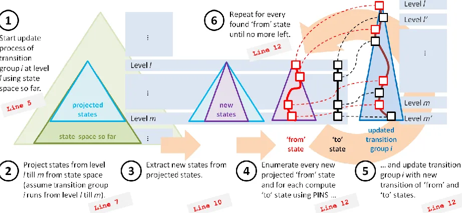
Figure 4.4: Pictorial overview of update process for transition group i with topmost level l (line numbers in figure refer to corresponding line numbers in Listing 4.3). ... 65

Figure 4.5: Different local state values located in different subtrees of reachable state space. ... 65

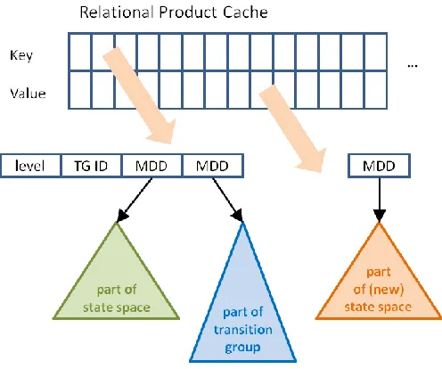
Figure 4.6: Visualization of the key and value used in the lookup table from the relational product... 66

Figure 4.7: Pictorial overview of using a bad key for the lookup table from the relational product. ... 67

Figure 4.8: Passing on calls of vset_least_fixpoint in spec-reach.c to atermdd.c. ... 68

Figure 4.9: Passing on calls related to update process of transition groups between spec-reach.c and atermdd.c. ... 69

Figure 5.1: Plot comparing time values between options no-sat and sat-ciardo. ... 79

Figure 5.2: Plot comparing time values between options sat-like and sat-ciardo. ... 80

Figure 5.3: Plot comparing time values between options no-sat and sat-ddd. ... 81

Figure 5.4: Plot comparing time values between options sat-like and sat-ddd. ... 82

Figure 5.5: Plot comparing time values between options sat-ddd and sat-ciardo. ... 83

Figure 5.6: Bar charts of peak MDD node values for each reachability option per DVE model. ... 84

Figure 5.7: Visualization of state and MDD count process used in option sat-ciardo. ... 85

(10)

10

Figure 5.9: State space evolution plots of DVE model anderson.6. ... 86

Figure 5.10: State space evolution plots of DVE model cambridge.7. ... 87

Figure 5.11: State space evolution plots of DVE model iprotocol.7. ... 88

Figure 5.12: Bar charts showing the contribution of useful and useless MDD projections using the reachability tools from LTSmin for 3 DVE model. ... 91

Figure 6.1: Pictorial overview of update process for all affected transition groups (line numbers in figure refer to corresponding line numbers in Listing 6.1). ... 99

Figure 6.2: Plots comparing time values between options no-sat and new sat-ciardo (left), and between options sat-like and new sat-ciardo (right). ... 104

Figure 6.3: Plots comparing time values between options sat-ddd and new sat-ciardo (left), and between options sat-ciardo and new sat-ciardo (right). ... 105

Figure A. 1: Plot comparing maximum memory values between options no-sat and sat-ciardo. ... 119

Figure A. 2: Plot comparing maximum memory values between options sat-like and sat-ciardo. ... 120

Figure A. 3: Plot comparing maximum memory values between options sat-ddd and sat-ciardo. ... 121

Figure A. 4: Plot comparing maximum memory values between options no-sat and sat-ddd. ... 122

Figure A. 5: Plot comparing maximum memory values between options sat-like and sat-ddd. ... 123

Figure A. 6: Plot comparing maximum memory values between options no-sat and new sat-ciardo. ... 124

Figure A. 7: Plot comparing maximum memory values between options sat-like and new sat-ciardo. ... 125

Figure A. 8: Plot comparing maximum memory values between options sat-ddd and new sat-ciardo. .... 126

Figure A. 9: Plot comparing maximum memory values between options sat-ciardo and new sat-ciardo. 127 Figure B. 1: State space evolution plots of DVE model at.5. ... 129

Figure B. 2: State space evolution plots of DVE model at.6. ... 130

Figure B. 3: State space evolution plots of DVE model bakery.6. ... 131

Figure B. 4: State space evolution plots of DVE model brp.5. ... 132

Figure B. 5: State space evolution plots of DVE model brp.6. ... 133

Figure B. 6: State space evolution plots of DVE model collision.4. ... 134

Figure B. 7: State space evolution plots of DVE model elevator_planning.2. ... 135

Figure B. 8: State space evolution plots of DVE model firewire_link.5. ... 136

Figure B. 9: State space evolution plots of DVE model iprotocol.6. ... 137

Figure B. 10: State space evolution plots of DVE model lamport.7. ... 138

Figure B. 11: State space evolution plots of DVE model lamport.8. ... 139

Figure B. 12: State space evolution plots of DVE model lamport_nonatomic.5. ... 140

Figure B. 13: State space evolution plots of DVE model lann.6. ... 141

Figure B. 14: State space evolution plots of DVE model lann.7. ... 142

Figure B. 15: State space evolution plots of DVE model leader_election.6. ... 143

Figure B. 16: State space evolution plots of DVE model leader_filters.7. ... 144

Figure B. 17: State space evolution plots of DVE model peterson.6. ... 145

Figure B. 18: State space evolution plots of DVE model peterson.7. ... 146

Figure B. 19: State space evolution plots of DVE model phils.6. ... 147

(11)

11

Figure B. 21: State space evolution plots of DVE model schedule_world.3. ... 149

Figure B. 22: State space evolution plots of DVE model szymanski.5. ... 150

Figure B. 23: State space evolution plots of DVE model telephony.4. ... 151

Figure B. 24: State space evolution plots of DVE model telephony.7. ... 152

Figure C. 1: Bar charts showing the contribution of useful and useless MDD projections using the reachability tools from LTSmin for 8 DVE model (1). ... 153

List of listings

Listing 1.1: Pseudo code of breadth-first search algorithm using newly unexplored states only (left) or all states (right). ... 16

Listing 1.2: Pseudo code of chaining algorithm using newly unexplored states only (left) or all states (right). ... 16

Listing 1.3: Variables and function definitions for pseudo code in previous two listings. ... 16

Listing 2.1: Pseudo code of Kronecker Prebuilt Saturation algorithm with additional code for On-the-fly version highlighted in light-blue [10]. ... 26

Listing 2.2: Function definitions used in pseudo code of Kronecker Saturation algorithms. ... 27

Listing 2.3: Pseudo code of confirmation process for updating events in Kronecker On-the-fly Saturation algorithm [10]. ... 29

Listing 2.4: Pseudo code of General Prebuilt Saturation algorithm with additional code for On-the-fly version highlighted in light-blue [23]. ... 33

Listing 2.5: Pseudo code of confirmation process for updating events in General On-the-fly Saturation algorithm [23]. ... 34

Listing 3.1: Pseudo code of basic sat-like algorithm and accompanying function definitions. ... 49

Listing 3.2: Pseudo code of sat-ddd algorithm. ... 50

Listing 4.1: Pseudo code of implemented General Prebuilt Saturation algorithm with additional code for On-the-fly version highlighted in light-blue and for revised On-the-fly version in dark-blue (which is discussed in chapter 6). ... 58

Listing 4.2: Function definitions used in pseudo code of implemented General Saturation algorithm. ... 59

Listing 4.3: Pseudo code of update process for updating a single transition group in implementation of General On-the-fly Saturation algorithm. ... 64

(12)

12

List of tables

Table 2.1: Kronecker product of next-state function in matrix form. ... 22

Table 2.2: Subcategories of Kronecker Saturation approaches. ... 22

Table 2.3: Example model 1 with a Kronecker-consistent next-state function. ... 22

Table 2.4: Bottom- and topmost levels for each event e of example model 1. ... 24

Table 2.5: Differences in implementation details between Kronecker Prebuilt and Kronecker On-the-fly Saturation. ... 30

Table 2.6: Subcategories of General Saturation approaches. ... 30

Table 2.7: Example model 2 with a general next-state function. ... 31

Table 2.8: Partitioning of events in enabling and updating conjuncts for example model 2. ... 31

Table 2.9: Differences in implementation details for General Prebuilt and General On-the-fly Saturation. 35 Table 3.1: Selection of command pre- and suffixes of state space exploration tools of LTSmin toolset. .... 40

Table 3.2: Some PINS operations and their arguments as defined in header file greybox.h (simplified). ... 43

Table 3.3: Example evaluation of PINS operations for example model 2. ... 43

Table 3.4: Available MDD data encodings in the LTSmin toolset. ... 45

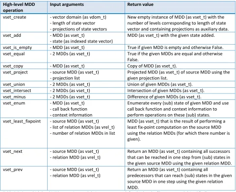
Table 3.5: Some high-level MDD operations and their arguments as defined in header file vector_set.h (simplified). ... 47

Table 3.6: Some high-level MDD operations and their arguments for transition groups as defined in header file vector_set.h (simplified). ... 47

Table 3.7: Some global variables used by reachability tools as defined in file spec-reach.c (simplified). .... 48

Table 3.8: Operation used by reachability tools as defined in file spec-reach.c (simplified). ... 48

Table 4.1: LTSmin-related requirements. ... 53

Table 4.2: Saturation-related requirements. ... 54

Table 5.1: Input arguments used with dve2-reach tool for experiments. ... 74

Table 5.2: DVE models used for experiments (with descriptions from BEEM database [20]). ... 75

Table 5.3: Overview of data that is being collected in the experiments using reachability tools from LTSmin. ... 75

Table 5.4: Experimental time results using the reachability tools from LTSmin on the 27 DVE models. ... 77

Table 5.5: Summary of the best and worst performing reachability options regarding time performance. 78 Table 5.6: Statistics showing the number of useful and total MDD projections made using the reachability tools from LTSmin on the 27 DVE models. ... 90

Table 5.7: Summary of the average percentage of useful MDD projections made per reachability option. 90 Table 5.8: Statistics from profiling using option sat-ciardo... 91

Table 5.9: Most demanding function for DVE models from Table 5.8. ... 91

Table 5.10: PINS dependency matrices for DVE models iprotocols.6 and iprotocols.7. ... 92

Table 6.1: Assumptions made for redesign of update process of General On-the-fly Saturation algorithm. ... 97

(13)

13

Table 6.3: Summary of the best and worst performing reachability options regarding time performance, including option new sat-ciardo. ... 101 Table 6.4: Statistics showing the difference in state space evolution of option new sat-ciardo compared to the previous version of option sat-ciardo (only for DVE models where a difference is noticed). ... 102 Table 6.5: Part of state space evolution of DVE model anderson.6 per iteration of Saturation at topmost working MDD level. ... 103 Table 6.6: Statistics showing the minimum and maximum growth of transition groups of 24 DVE models for option new sat-ciardo compared to previous version of option sat-ciardo. ... 106

(14)

(15)

15

1 Introduction

Real-life critical software systems are developed with reliability and correctness in mind. During the development of such systems formal verification can play an important role. In formal verification the system under development is abstracted into a model which is checked against the given specifications to assess any errors and design flaws that may occur. One of such formal verification techniques is model checking and tools exist which are capable of automatically performing such verification on formal properties (which are the formalizations of the given specifications). Such tools basically assess these properties by considering all states of the model reachable from the initial state(s), which is referred to as state space generation or reachability analysis. The tool exhaustively searches all possible reachable states of the model using a transition relation or next-state function of the model. The latter indicates how a model can undergo a transition from one state to another. A major hurdle here is the inability to deal with large complex models containing billions of states.

Traditionally two approaches have been used for state space generation [7]:

■ Explicit state space generation: states are found individually and stored explicitly one-by-one. ■ Implicit or symbolic state space generation: multiple states are found and stored together in sets.

Unfortunately, both approaches suffer from the state space explosion problem in which case it becomes infeasible in both time and memory to compute the reachable state space when the system model becomes larger and more complex. The number of states that can be handled with the explicit approach lies roughly around 107 states [7] and this is mainly due to the problem that time and space complexity increase linearly with increasing reachable state space (when considering the fact that the exploration happens in a sequential manner). The symbolic approach can handle reachable state spaces up to approximately 1020 states [7] when the sets of states are stored using Binary Decision Diagrams (BDDs). This encoding is also used for storing the transition relations, so operations on BDDs are mainly affected by the number of nodes in the BDDs. The main challenges of the symbolic approach [7] are as follows:

■ The maximum number of BDD nodes handled and stored, is called the peak BDD size and may require an excessive amount of memory that is not available, although the final BDD size can be quite

compact.

■ Handling BDDs as one rigid structure can be infeasible when they are very large and complex. Partitioning techniques can be used that partition the transition relation in more manageable subrelations or events. Conjunctive partitioning is used for synchronous system models, since the transition relation TR can be viewed as a conjunction of N individual events Ei, denoted as TR = E1 ∧ E2 ∧ … ∧ EN. Similarly disjunctive partitioning is used for asynchronous system models, where the transition relation TR is a disjunction of N individual events Ei, denoted as TR = E1 ∨ E2 ∨ … ∨ EN. Also combinations of these partitioning techniques occur. The main challenge is to find a suitable and manageable partitioning for the transition relation.

(16)

16

When comparing breadth-first search and chaining, the latter appears to be a better traversal approach [10]. But for real-life complex system models, both approaches are still unable to handle extremely large state spaces. Next to these two approaches, a relatively new technique for traversing a state space of a system model has emerged to tackle this problem. This approach is called Saturation, which is developed by G. Ciardo [8]. It has proven itself as a good competitor to traditional symbolic state space generation techniques for handling models with extremely large state spaces and different versions of the approach have been devised.

1 2 3 4 5 6 7 8 9 10 11 12 13

set<state> visited := { init } set<state> current := visited set<state> next_set := { } set<state> tmp := { }

while (current != { }) : next_set := { }

foreach (int i in 1..evts.length() : tmp := next(current, evts[i]) tmp := tmp - visited

next_set := next_set + tmp visited := visited + next_set current := next_set

1 2 3 4 5 6 7 8 9

set<state> visited := { init } set<state> old_vis := { } set<state> tmp := { }

while (visited != old_vis) : old_vis := visited

foreach (int i in 1..evts.length) : tmp := next(old_vis, evts[i]) visited := visited + tmp

Listing 1.1: Pseudo code of breadth-first search algorithm using newly unexplored states only (left) or all states (right).

1 2 3 4 5 6 7 8 9 10 11

set<state> visited := { init } set<state> new_set := visited set<state> tmp := { }

while (new_set != { }) :

foreach (int i in 1..evts.length) : tmp := next(new_set, evts[i]) tmp := tmp - visited

new_set := new_set + tmp visited := visited + new_set new_set := new_set – visited

1 2 3 4 5 6 7 8 9

set<state> visited := { init } set<state> old_vis := { } set<state> tmp := { }

while (visited != old_vis) : old_vis := visited

foreach (int i in 1..evts.length) : tmp := next(visited, evts[i]) visited := visited + tmp

Listing 1.2: Pseudo code of chaining algorithm using newly unexplored states only (left) or all states (right).

1 2 3 4 5 6 7 8 9 10 // Variables:

// Initial state of model.

state init

// List containing all events (partitioned transition relations).

array<event> evts

// Function:

// Compute next (successor) states starting from from_states using event evt.

set<state> next(set<state> from_states, event evt)

Listing 1.3: Variables and function definitions for pseudo code in previous two listings.

The indices of arrays are numbered from 1 to length.

‘set + set’ = set union ‘set – set’ = set difference

(17)

17

1.1 Goal statement

The Formal Methods and Tools (FMT) research group at the University of Twente has developed its own verification toolset called LTSmin which is the result from years of research and includes a tool for symbolic model checking [5]. It contains a clean medium for representing the states of a model in a uniform way where an interface, called PINS is used [4]. Using this interface the LTSmin toolset is capable of separating the language specific details of modelling languages, from the model checking algorithms used for verification. The tool implements several symbolic reachability algorithms, such as breadth-first search and chaining. Also LTSmin versions of Saturation-like algorithms are implemented, but these have not yet been compared with those by G. Ciardo.

The aim is to extend the symbolic reachability algorithms in the LTSmin toolset with the Saturation-based approach by G. Ciardo. The approach should be incorporated in the tool with its architecture and PINS interface in mind, and should maintain the benefits of keeping the algorithm independent from any language module. Basically the tool should eventually be capable of using Saturation as reachability technique for state space generation of any model that the tool can handle.

The main goal of this project is summarized as follows:

“Design and assess a Saturation-based approach as devised by G. Ciardo for the LTSmin toolset.”

To achieve the given goal, the following research questions provide guidance in this project:

■ “Different versions of the Saturation approach exist and which one of these is a good candidate for extending the symbolic reachability techniques of the LTSmin toolset?”

■ ”How can the chosen version of the Saturation approach be implemented in the LTSmin toolset and what are the consequences for the tool’s architecture?”

■ “How does the chosen Saturation approach perform in the LTSmin toolset compared to other symbolic reachability techniques in the tool?”

1.2 Document structure

The report follows the research questions to reach the main goal of this project. Chapter 2 gives an overview of the different Saturation approaches that exist and how they evolved over time. It will provide a basis for the first research question. Chapter 3 explains the architecture of the LTSmin toolset and the main focus lies with parts of the toolset that deal with reachability analysis. This will provide a basic understanding of how the LTSmin toolset is set up for answering the second research question. Chapter 4 gives an answer to the first two research questions by discussing the underlying choice of the Saturation approach to implement and how the algorithm can be incorporated in the LTSmin toolset. It also

continues with discussing the issues that arise during actual implementation in the LTSmin toolset and how these are solved (relating to the second research question as well). Chapter 5 finalizes the

implementation of the chosen Saturation approach by evaluating its performance, as indicated in the third research question. But the report does not end here and continues with an improvement on the

implemented Saturation approach in chapter 6. This chapter discusses the design, implementation and evaluation of an improved version of the implemented Saturation approach and will therefore also contribute to the third research question. The report ends in chapter 7 with how the main goal of

(18)

(19)

19

2 Overview of Saturation approaches

This chapter starts with basic definitions of state spaces and next-state functions (or transition relations) of system models. Section 2.2 and 2.3 each give an overview of one of the two main categories of the Saturation approaches as devised by G. Ciardo.

2.1 Definitions and encodings for state space and next-state function

A discrete-state model is used for encoding a model of the system under consideration [10][7]. Definition 2.1. A discrete-state model is a tuple

(Ŝ, N, S

init

₎

_{[7], where}

■

Ŝ

is the set of all possible states

i

of the system (reachable or not);

■

N: Ŝ → 2

Ŝ _{is the next-state function,}

_N(i)

_{consists of all states reachable in one step from}

_i

_;

■

S

init

⊆

_Ŝ

_{is the set of initial states.}

For discussing the Saturation approaches, the set

S

init

will only contain a single initial state and the approaches can be extended to multiple initial states. The set of reachable states of the system is denoted by

S ⊆ Ŝ

.

The model is usually decomposed into a number of

K

components and a model’s state

i

is a vector written as a

K

-tuple

(iK, …, i1)

with

Ŝ = SK × … × S1

and

il ∊ Sl

for all 1 ≤ l ≤ K. Each state slot

il

in the state vector corresponds to a local state of the corresponding component

l

. For convenience, the local states of a component

l

are assumed to be integer values ranging from 0 to

nl – 1

, with

nl

the size of the local state space of component

l

[10].

When the discrete-state model uses

K

variables in its specification and a model’s state consists of

enumerating the values of these

K

variables (corresponding to the Cartesian product

SK × … × S1

), then a state slot in a state vector corresponds to one of these

K

variables (one of the elements of the Cartesian product). The variables are ordered in a predefined way (mostly as part of the model’s specification) and the local state space sizes correspond to the domains of these variables.

For every Saturation approach the state space is stored as a quasi-reduced

K

-level Multi-valued Decision Diagram [10]. They are almost similar to BDDs, but instead of 2 outgoing arcs per node, each node contains

nl

outgoing arcs. Each level l corresponds to the accompanying component

l

of the model. The next-state function is stored in different ways for different Saturation approaches and is discussed later. Mostly it is not stored in a single rigid data structure, but split into smaller manageable parts.

Definition 2.2. A quasi-reduced

K

-level Multi-valued Decision Diagram (abbreviated to MDD) is a directed acyclic edge-labelled multi-graph [7], where:

■ Nodes are put into levels ranging from

K

to 0 (i.e.

K + 1

levels).

■ Level

K

contains a single non-terminal root node

r

and one or more non-terminal nodes are situated at levels

K – 1

to 1.

(20)

20

A path starting from the root node of an MDD and ending in the True node indicates a reachable state of the model. The MDD as defined above is not used as such, since this would also store the MDD nodes of unreachable states and the False MDD node. In practice, a reduced version of this MDD is stored,

containing only the reachable states. That redundant MDD nodes are stored, is an artefact of building the MDD level by level from the bottom-up by the Saturation algorithm (more about this in section 2.2.1). ■ From model to MDD example

To give a sense what an MDD of a reachable state space looks like, consider one has a model specification and that the entire model itself can be decomposed into 5 smaller components which interact with each other in a certain way (so

K

= 5), as shown on the left in Figure 2.1. Another representation is that the model is specified using 5 variables and each is defined by a (mathematical) function, as shown on the right in Figure 2.1. A state vector of this model is written as a 5-tuple

(i5, i4, i3, i2, i1)

with

Ŝ = S5 × S4 × S3 ×

S2 × S1

. Each component has its own local state space size

nl

and the values of the local state spaces are

given on the right in Figure 2.2 (and likewise for the domain of the 5 variables of the model).

Furthermore imagine the model can have a set of reachable states

S

as given on the left in Figure 2.2 and this set is stored in an MDD, as depicted in the two MDDs. The left MDD stores every single state of the model and each MDD node has

nl

outgoing arcs (according to Definition 2.2), while the right MDD only stores the reachable states of the model.

A path starting from the root node at level 5 to the True MDD node at level 0 represents a reachable state of the model. So for state (0, 3, 1, 0, 1) one would start at the root node (at level 5) and take the arc pointing out of entry value 0. Arriving at the MDD node at level 4, one needs to take the arc heading out of entry value 3 to the next MDD node at level 3, and so on until the True MDD node at level 0.

The MDDs do not contain duplicate nodes, since there are no two MDD nodes with the same entry values and that have the same set of incoming and outgoing arcs (pointing to the same set of MDD nodes).

Figure 2.1: Example of a model represented as a decomposition (left) and as a function (right).

(21)

21

2.2 Saturation approaches for Kronecker-consistent models

The first group of Saturation approaches require that the decomposition of the next-state function is Kronecker consistent, meaning that the effect of an event

e

on component

l

only depends on its

corresponding local state space. Thus, it is possible to find

K ∙ |E|

subfunctions

Nl,e

, where

E

denotes the set of events. Some modelling formalisms such as basic Petri Nets satisfy this property automatically, but this is not always the case. In these other cases, one can still obtain a Kronecker-consistent decomposition of the next-state function by splitting and/or combining events, or performing these operations on the model components. This needs to be done manually before providing the model to the Saturation algorithm, because currently there is no technique available that can handle this automatically for every general type of model (it can for certain types of Petri Nets as implemented in the research tool SMART by G. Ciardo [7][6]).

The next-state function is represented as a Kronecker product on Boolean adjacency matrices. A Kronecker product on two matrices is defined below.

Definition 2.3. Kronecker product (or matrix direct product) of two matrices [25]. ■ Given: m × n matrix A and p × q matrix B

■ Result: (mp) × (nq) matrix C with elements cxy = aijbkl, where x ≡ p(i – 1) + k and y ≡ q(j – 1) + l.

■ Notation: C = A

⊗

B

Basically, the Kronecker product on two matrices is a form of matrix multiplication, where intuitively each value of matrix A is multiplied with the entire matrix B. Take for example the Kronecker product of a 1 × 3 matrix A and a 2 × 3 matrix B, which results in a 2 × 9 matrix C, as shown in Figure 2.3.

Figure 2.3: Example of Kronecker product for a 1 × 3 matrix A and a 2 × 3 matrix B.

(22)

22

Events

1

2 …

e

…

n

Levels

K

NK,1

NK,2

…

NK,e

…

NK,n

K – 1

NK – 1,1

NK – 1,2

NK – 1,e

NK – 1,n

...

_…

l

Nl,1

Nl,2

Nl,e

Nl,n

…

2 N2,1

N2,2

N2,e

N2,n

1 N1,1

N1,2

…

N1,e

…

N1,n

Table 2.1: Kronecker product of next-state function in matrix form.

An advantage of storing the next-state function in this manner, is that the submatrices

Nl,e

are quite sparse. Moreover, if the occurrence of certain events do not affect the local state space of a component

l

, then the submatrix

Nl,e

is simply the identity matrix and can be stored more efficiently [10].

In the following subsections two variants of this group of Saturation approaches will be discussed in detail, as summarized in Table 2.2. For convenience, they will be denoted as Kronecker Saturation approaches from now on.

Kronecker Saturation approaches

Name Kronecker Prebuilt Saturation Kronecker On-the-fly Saturation

Explanation Next-state function is Kronecker consistent and is built in advance (prebuilt) before starting the Saturation process.

(Local state space sizes nl are known.)

Next-state function is Kronecker consistent and built on-the-fly during the Saturation process.

(Local state space sizes nl are unknown.)

Table 2.2: Subcategories of Kronecker Saturation approaches.

■ Running example 1 – Model description

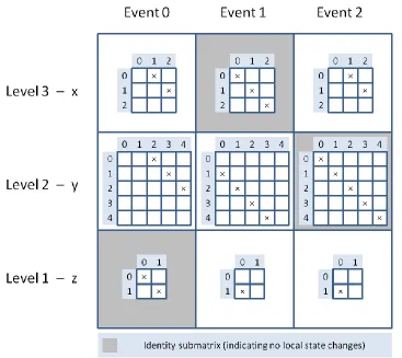
As a running example for Kronecker Saturation throughout this report, a simple program model is used which consists of three (interleaving) parallel processes and three global variables x, y and z. To obtain a Kronecker-consistent next-state function, the individual updating statements (not conditions) of the processes can only rely on at most a single variable, namely their own variable. Each process is considered to consist of a single event and the three variables x, y and z correspond to level 3, 2 and 1 of the MDD, respectively. An overview of the program model is given below in Table 2.3.

Level Variable Initial value Local state space Event Process of program

3 x 0 S3 = {0, 1, 2} 0 if x < 2 and y < 3 then

{ x = x + 1 ; y = y + 2 ; }

2 y 0 S2 = {0, 1, 2, 3, 4} 1 if y > 0 and z > 0 then

{ y = y – 1 ; z = z – 1 ; }

1 z 1 S1 = {0, 1} 2 if x < 2 and z > 0 then

(23)

23

■ Running example 1 – Kronecker matrix of next-state function

[image:23.612.72.439.153.480.2]

Following example model 1, the submatrices

Nl,e

per level and event of the entire next-state function can be determined, which is shown in (Kronecker) matrix form in Figure 2.4. So the entire matrix depicted forms the Kronecker product of the complete next-state function

N

and each (large) matrix cell contains a Boolean adjacency matrix

Nl,e

(for readability reasons crosses are used to indicate the value True and empty cells indicate the value False).

Figure 2.4: Kronecker product of next-state function in matrix form for example model 1.

2.2.1 Kronecker Prebuilt Saturation approach

The most basic version of the Kronecker Saturation approach is first presented in [8] and later more extensively discussed in [10] and [7]. Next to the requirement of Kronecker consistency of the next-state function, this version of the Saturation algorithm also requires that

nl

, the local state space size of component

l

, is known in advance. With this knowledge, it is easier to map local states to their

corresponding local state values (ranging from 0 to

nl – 1

). And with the known local state space sizes, the next-state function can be prebuilt as a Kronecker product of Boolean adjacency matrices

Nl,e

before generating the reachable state space using Saturation. Therefore this variant of the Kronecker Saturation approach will be denoted as Kronecker Prebuilt Saturation.

(24)

24

range of levels can be determined in which the local states of the corresponding levels undergo a

transition to another local state and these are indicated with the top- and bottommost levels per event

e

, respectively

Top(e)

and

Bot(e)

. Levels above and below this range are not affected by event

e

, since these only contain identity transitions. For the Saturation algorithm, this means that in a level

l

an event

e

is only fired when it falls within the range between

Top(e)

and

Bot(e)

, avoiding unnecessary firings where the local state space remains the same. Hereby the entire set of events

E

is partitioned into event sets per level

l

, namely

ℰl = { e ∊ ℰ: Top(e) = l }

.

In the traditional symbolic approach the unsaturated BDD nodes found, are mostly immediately replaced by (a number of) new BDD nodes that encode a larger set of states [7]. The number of unsaturated nodes is very unpredictable and changes all the time, which contributes largely to the peak BDD size. This is avoided in the Saturation algorithm by getting rid of unsaturated nodes as early as possible.

■ Running example 1 –

Bot(e)

and

Top(e)

In Table 2.4

Bot(e)

and

Top(e)

of the three events are shown for example model 1. So for example the bottommost level for event 0 is level 2 and this means that every submatrix

Nl,e

below level 2 of event 0 are just identity matrices (containing only identity transitions). And

this is similar for the topmost level, but then for submatrices

Nl,e

above the topmost level.

The submatrices within the range of

Bot(e)

and

Top(e)

for a certain event

e

can still contain identity submatrices, as is the case with event 3, as can be seen in Figure 2.4.

The resulting Kronecker Prebuilt Saturation algorithm is described in [8], [10] and [7] (although these papers show some minor differences in the pseudo code, the basic structure of the algorithm is the same). The Saturation algorithm consists of three main functions, namely generate, saturateand fire. The function generate_{has as main purpose to create an empty MDD node for a state slot at level}

_l

_{of the}

initial state vector and saturate it by calling the function saturate. After this MDD node has been saturated, the next state slot of the initial state vector is handled until no more state slots are left. The function saturate is used to saturate an MDD node on a certain level

l

. It tries to fire every possible event from the set

El

(iterating over this event set), where MDD nodes on lower levels are turned into saturated ones per event. Hereby the current MDD node is only updated in-place if new (local) states are discovered. In this case every event from the set

El

needs to be iterated over and fired again to check if it is possible to discover more reachable states. Finally the updated MDD node is placed in the unique (lookup) table.

The function fire is almost similar to the previous function, but only saturates lower-level MDD nodes for a particular event

e

and this function is called only with an MDD node on levels lower than

Top(e)

. It traverses down the MDD until

Bot(e)

is reached, if a certain MDD node and event combination has been handled before, or if no more successors are found. Before unwinding out of the recursive calls of fire, any newly found states are saturated as well with the function saturate. Basically function fire

calculates the next (local) states or relational product for a certain MDD.

So for a given model, after creating an empty MDD node for a state slot (at level

l

) of the initial state vector, this MDD node is saturated by considering all events from the set

El

. It then fires each event separately by traversing the MDD downwards (by calculating the relational product) and saturating it on the way from the bottom-up when returning back to the MDD node it started with. Saturation is then repeated for the same events if new (local) states are found. Otherwise the whole process is repeated for

Event

e

Bot(e)

Top(e)

0 Level 2 Level 3

1 Level 1 Level 2

2 Level 1 Level 3

(25)

25

the next state slot of the initial state vector until the last state slot of the initial state vector is saturated and the result is the reachable state space of the given model.

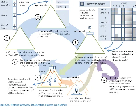
The pseudo code of the described functions can be found in Listing 2.1 (for now the highlighted parts can be safely ignored). Furthermore Listing 2.2 provides some explanations for a couple of operations on MDD nodes. Figure 2.5 gives a pictorial overview of the described Saturation process, and some definitions regarding the working MDD level are explained in Figure 2.6, which indicates the current working level for which a Saturation process is started for events that start at a topmost level.

[image:25.612.71.542.180.557.2]

Figure 2.5: Pictorial overview of Saturation process in a nutshell.

(26)

26 1 2 3 4 5 6 7 8 9 10 11 12 13 14 15 16 17 18 19 20 21 22 23 24 25 26 27 28 29 30 31 32 33 34 35 36 37 38 39 40 41 42 43 44 45 46 47 48 49 50 51 52 53 54

// Generate MDD tree of reachable state space, starting from initial state.

MDDnode generate(array<int> init_vector) : MDDnode p := getMDDTrue()

for (int level in 1 .. init_vector.length()) :

i := getAllStateValsOfLevel(level).add(init_vector[level])

confirm(level, i)

MDDnode r := createEmptyMDD(level)

r.setArc(init_vector[level], p) // On-the-fly: r.setArc(i, p)

p := saturate(level, r) return p

// Saturate MDD subtree in a certain level.

MDDnode saturate(int l, MDDnode p) :

set<event> topLvlEvts := getEventsOnTopLevel(l) while (! topLvlEvts.empty() ) :

event evt := topLvlEvts.pickEvent()

foreach (int i in getLocalStateVals(evt, l, p)) : MDDnode f := fire(evt, l - 1, p.getArc(i)) foreach (int j in getNextStates(evt, l, i)) : MDDnode u := unionMDDs(l - 1, f, p.getArc(j)) if (u != p.getArc(j)) :

if (! getAllStateValsOfLevel(l).contains(j)) :

confirm(l, j) p.setArc(j, u)

topLvlEvts := getEventsOnTopLevel(l) return checkMDDnode(UT[l], p)

// Fire event on MDD subtree in a certain level // for finding new MDD subtrees to saturate.

MDDnode fire(event evt, int l, MDDnode q) : if (l < getBottomLevelForEvent(evt)) : return q

MDDnode s := findInLookupTable(FC[l], (q, evt)) if (s != null) :

return s

s := createEmptyMDD(l)

foreach (int i in getLocalStateVals(evt, l, q)) : MDDnode f := fire(evt, l - 1, q.getArc(i)) foreach (int j in getNextStates(evt, l, i)) :

if (! getAllStateValsOfLevel(l).contains(j)) :

confirm(l, j)

s.setArc(j, unionMDDs(l - 1, f, s.getArc(j))) s := saturate(l, s)

insertInLookupTable(FC[l], (q, evt), s) return s

// Return set of (local) state slot values for which a certain event can fire // in a certain level for MDD subtree.

set<int> getLocalStateVals(event evt, int l, MDDnode p) : set<int> localStateVals

foreach (int i in getAllStateValsOfLevel(l)) :

if (p.getArc(i) != getMDDFalse() && ! getNextStates(evt, l, i).empty()) : localStateVals.add(i)

return localStateVals

Listing 2.1: Pseudo code of Kronecker Prebuilt Saturation algorithm with additional code for On-the-fly version highlighted in light-blue [10].

Function in pseudo code Notation

getEventsOnTopLevel(l)

_El

getNextStates(alpha, l, i)

_Nl,α(i)

getBottomLevelForEvent(alpha)

_Bot(α)

getAllStateValsOfLevel(l)

_Sl

The indices of arrays are numbered from 1 to length().

Global lookup tables (per level)

(27)

27 1 2 3 4 5 6 7 8 9 10 11 12 13 14 15 16 17 18 19 20 21 22 23 24

// Create a new empty MDD node at the given level.

MDDnode createEmptyMDD(int level)

// Check if the given MDD tree is already stored in the given lookup table. If so, // the value from the lookup table is returned, otherwise the given MDD tree is // inserted into the lookup table and returned.

MDDnode checkMDDnode(array<MDDnode> lookup_table, MDDnode set)

// Return MDD node pointed to by arc belonging to the given local state value. // If current MDD node does not contain the given local state value, then the False // MDD node is returned.

MDDnode getArc(int value)

// Set arc (belonging to the given local state value) to point to the given MDD // node. If current MDD node does not contain the given local state value, then // insert a new entry with this local state value and set the arc to the given MDD // node.

void setArc(int value, MDDnode set)

// Return the True MDD node.

MDDnode getMDDTrue()

// Return MDD tree of given state vector (consisting of integer state values).

MDDnode getInitMDD(array<int> state_vector)

Listing 2.2: Function definitions used in pseudo code of Kronecker Saturation algorithms.

2.2.2 Kronecker On-the-fly Saturation approach

In [9] an extension to the Kronecker Prebuilt Saturation approach is described which lifts the requirement that the local state space sizes

nl

are known in advance. It turns out that when

nl

is determined for each component

l

beforehand, one can encounter either an infinite value for the local state space or spurious states (in which case

nl

may be larger than necessary). Manually manipulating the model in advance to cope with this issue is not a good solution, due to newly introduced (human) errors.

The next version of the Saturation algorithm deals with two issues in parallel, namely determining the smallest size of each local state space and generating the reachable state space of the model. In this algorithm new locally reachable states are discovered and only those that are also globally reachable are stored by indicating that they are confirmed to occur in the reachable state space. So it is only viable to consider transitions originating from confirmed local states, and ignoring the ones starting from unconfirmed local states. For this to work, the algorithm needs to keep track of the possible firings of events starting from these confirmed states (and this also explains the name On-the-fly Saturation, since it discovers (local) transitions on-the-fly). This is done by incrementally building the next-state function (as before as Boolean adjacency matrices

Nl,e

) to keep track of which firings of events are possible. In the Prebuilt version of the Saturation algorithm the submatrices

Nl,e

are prebuilt and are always square-shaped. But now they are generated on-the-fly, these submatrices mostly have a rectangular size during its evolution with the rows corresponding to confirmed local state values and the columns to both confirmed and unconfirmed local state values (these local state values are discovered with the confirm

function, as will be explained below). At the end of its evolution some submatrices

Nl,e

can end up in a square shape, meaning that all available local state values are globally reachable.

(28)

28

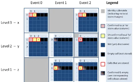
■ Running example 1 – Fictitious on-the-fly confirmation of next-state function

The initial state values are confirmed one by one, but if all initial state values would be confirmed at the beginning, then the Kronecker product of the next-state function would look in (Kronecker) matrix form like the one as depicted in Figure 2.7. Only one row of each adjacency submatrix has been discovered here and the cells in the row until the local state transitions (indicated by crosses) are stored (so the adjacency submatrices have a rectangular shape).

[image:28.612.74.542.274.564.2]

When one of the local state transitions to an unconfirmed local state is taken (cross located in a yellow cell), confirm is called first to confirm the row in all submatrices at the same level corresponding to the local state to which it is going to by the local transition. So take for example the submatrix

N3,0

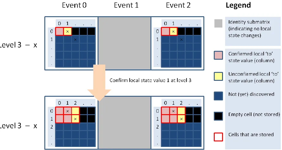
for level 3 and event 0. Before a transition is performed from local state value 0 to local state value 1 (indicated by cross), the row for local state value 1 needs to be confirmed first in all submatrices at level 3. During the confirmation, the rectangular shape of the submatrices is maintained. In this case the number of columns of the submatrix is increased from 2 to 3 as is shown in Figure 2.8.

(29)

[image:29.612.80.541.73.318.2]

29

Figure 2.8: Visualization of confirmation process for local state value 1 at level 3 (which only affect matrix cells at level 3) for example model 1.

The resulting Kronecker On-the-fly Saturation algorithm has basically the same structure as the Kronecker Prebuilt Saturation algorithm, but a new function confirm is added which is confirming newly found local state values [9][10]. This function basically looks for every Boolean adjacency matrix

Nl,e

where

l

corresponds to the current level. While iterating over each event

e

, for each submatrix

Nl,e

that is not equal to an identity transition (except when it lies in the range of

Bot(e)

and

Top(e)

), it adds a new row to this submatrix for the newly discovered local ‘from’ state value and extracts the local ‘to’ state values it heads to in this row. The local ‘to’ state values can contain both confirmed as unconfirmed local state values.

In practice the local state values are not discovered in numerical order from 0 to

nl

– 1. A more efficient way to add new rows to the submatrix

Nl,e

is to map the real local state value to the row index of the first occurring empty row in the submatrix. In this way new rows are added adjacently to the existing rows in submatrix

Nl,e

and the algorithm uses the mapped local state values in the algorithm.

The corresponding pseudo code of this function clarifies this in Listing 2.3, where the highlighted code segments indicate the use of mappings for the real local state values.

1 2 3 4 5 6 7 8 9 10 11 12 13 14

// Constant integer indicating that a certain mapping (for a key) does not exist.

constant int NULL_MAPPING := MIN_INTEGER

// Confirm the newly found (‘from’ local state) value at the given level and update // affected events by inserting new transitions using model specifications.

void confirm (int level, int from_value) :

int real_from_value := getInvMapping(from_value)

foreach (event evt with getNextStates(evt, level) != getIDMatrix(level)) :

foreach (real_to_value in getNextStatesFromModel(evt, level, real_from_value)) : int to_value := getMapping(real_to_value)

if (to_value != NULL_MAPPING) : to_value := createMapping()

setNextStates(evt, level, from_value, to_value) getAllStateValsOfLevel(level).add(from_value)

(30)

30

In the algorithm some additional function calls to confirm are added (see highlighted code in Listing 2.1). The confirmation in the function generate is obvious, because it needs to confirm the initial local state value at each level. The other two confirm functions are located at points when it is certain that a new local state value is globally reachable.

The difference between Kronecker Prebuilt and Kronecker On-the-fly Saturation algorithms in terms of implementation details of the next-state function is given in Table 2.5.

Kronecker Saturation algorithm

Prebuilt On-the-fly

Next-state function

Static and partitioned into Boolean matrices in advance. They are only read.

Dynamic and partitioned into Boolean matrices. They are created incrementally (during saturation) from a high-level transition spec and read.

Table 2.5: Differences in implementation details between Kronecker Prebuilt and Kronecker On-the-fly Saturation.

2.3 Saturation approaches for general models

In [11] and [23] the Saturation approach is further extended, by handling decompositions of the next-state function that are not Kronecker consistent and this gives us the second group of Saturation approaches. To handle these, the next-state function is partitioned using disjuncts over each occurring event and conjuncts representing the transitions that synchronously update several (local) states at once [11]. The conjuncts are divided to handle the following two cases:

■ A set of enabling conjuncts indicating when an event

e

can occur.

■ A set of updating conjuncts indicating how each local state can transition to another local state when event

e

occurs.

In [11] this distinction within conjuncts is made explicitly, but is not necessary when using this group of Saturation algorithms as explained in [23].

Now for the encoding of the next-state function, variants of MDDs are used which will be discussed per approach in the following subsections.

Just as the Kronecker Saturation approaches, two variants exist which will be discussed in the following subsections, as summarized in Table 2.6. For convenience, they will be denoted as General Saturation approaches from now on.

General Saturation approaches

Name General Prebuilt Saturation General On-the-fly Saturation

Explanation Next-state function from general types of models is built in advance (prebuilt) before starting the Saturation process.

(Local state space sizes nl are known.)

Next-state function from general types of models is built on-the-fly during the Saturation process.

(Local state space sizes nl are unknown.)

(31)

31 ■ Running example 2 – Model description

As a running example for general Saturation throughout this report, a simple program model is used which consists of three (interleaving) parallel processes and three global variables x, y and z. The next-state function does not need to be Kronecker-consistently decomposable and so the individual next-statements of the processes can rely on multiple variables (in this example at most two variables). Each process is considered to be an event and the three variables x, y and z correspond to level 3, 2 and 1 of the MDD, respectively. The program model is summarized below in Table 2.7.

Level Variable Initial values Local state space Event Process of program

3 x 0 S3 = {0, 1, 2} 0 if x < y then { x = x + 1 ; }

2 y 0 S2 = {0, 1, 2} 1 if y < 2 then { y = y + 1 ; }

1 z 0 S1 = {0, 1, 2} 2 z = x ;

Table 2.7: Example model 2 with a general next-state function.

■ Running example 2 – Disjunctive & conjunctive partitioning

The disjunctive partitioning of the transition relation of example model 2 is already given above: each event represents a disjunct. The conjuncts for each of these disjuncts would be as given in Table 2.8.

Event Enabling conjunct Updating conjunct

0 x < y x = x + 1

1 y < 2 y = y + 1

2 True z = x

Table 2.8: Partitioning of events in enabling and updating conjuncts for example model 2.

2.3.1 General Prebuilt Saturation approach

The General Prebuilt Saturation algorithm needs to know the local state space sizes (or variable domains) and the partitioned next-state function prior to running the Saturation algorithm, just as is the case with the Kronecker Prebuilt Saturation algorithm. Also the notions of node saturation, event locality and in-place updates are present in the General version of the algorithm. Compared to the Kronecker Saturation algorithms, the pseudo code of the General version of the algorithm is set up slightly different, but the main structure is still visible [23] (in [11] the pseudo code of the algorithm is given as well, but is written more abstractly). The General Saturation algorithm now consists of four main functions, namely

generate, saturate,doFixPoint and relProd.

The function generate is different from the one in the Kronecker Prebuilt Saturation algorithm in the sense that it creates the entire MDD of the initial state at once (for all initial state values), before starting the saturation process by calling saturate_.

The function saturate looks for successor MDD nodes of a given MDD node to saturate and to perform a fix-point computation on them, which is then stored in a unique (lookup) table. Prior to looking for

successor MDD nodes, it first checks if the given MDD node has been handled before.

The main work of saturating MDD nodes now lies with the function doFixPoint. Just as is the case in the function saturate of the Kronecker Prebuilt Saturation algorithm, it tries to saturate a given MDD node on a certain level

l

.

Saturation for LTSmin