Buoyant jets with two and three dimensional trajectories

(1)

BUOYANT JETS WITH TWO AND

THREE-DIMENSIONAL

TRAJECTORIES

A thesis

submitted in partial fulfilment

of the requirements for the Degree

of

Doctor of Philosophy in Civil Engineering

at the

University of Canterbury

by

Gustaaf Adriaan Kikkert

University of Canterbury

Christchurch, New Zealand

(2)

(3)

Abstract

Extensive experimental data is available from previous research into the behaviour of buoyant jets released into an unstratified ambient. The experimental data has been the basis for theoretical and numerical modelling work, and currently several numerical models exist that are employed in the design of engineering structures built for the disposal of wastewater in the ocean. However there are still flow configurations with limited or no available experimental data, and hence confidence in the use of the models under some circumstances is limited. These circumstances include two-dimensional trajectory flows that are discharged at oblique angles to the ambient and buoyant jet flows with three-dimensional trajectories. As part of the current project an experimental investigation is conducted into the behaviour of discharges that have either two-dimensional or three-dimensional trajectories, focussing particularly on those configurations with currently limited available experimental data.

A light attenuation technique is developed for the investigation of such flows, largely because it enables the behaviour of discharges with three-dimensional trajectories to be recorded with relative ease. However, this technique provides integrated views of the flow and hence the interpretation of the integrated concentration data is aided by assumed mean cross-sectional concentration profiles. In the strongly advected region (with the exception of the weak-jet) a double-Gaussian approximation is shown to provide a reasonable representation of mean concentration profiles. In the weakly advected regions and the weak-jet region, it is well-known that a single Gaussian adequately represents the mean flow structure.

A new numerical model, the Momentum Model, is developed to assist in the design and to monitor the performance of the experimental investigation. Unlike other models, the behaviour of the flow is determined by the relative magnitudes of the initial excess momentum flux, the buoyancy-generated momentum flux and the entrained ambient momentum flux. It is shown that ratios of these momentum fluxes are equivalent to the length-scales traditionally employed for this task.

(4)

buoyant jet discharged in a moving ambient show that the spreading rates of the strongly advected flows (puffs and thermals) differ, and while this difference is incorporated into the Momentum Model, it is not evident in the VisJet and CorJet predictions.

Numerical model predictions of negatively buoyant discharges are shown to be inadequate. This discharge configuration is investigated in some detail experimentally and additional analytical solutions of the flow behaviour are developed to aid in the interpretation of the flow behaviour. The experimental results show that buoyancy-induced instabilities on the inner side of the jets, which generate additional vertical mixing, significantly alter the form of the mean concentration profiles in this region. This results in considerably higher integrated dilutions along the flow centreline.

Another significant difference between the newly developed Momentum Model and the existing numerical models (VisJet and CorJet), is the approach taken to dealing with oblique discharges in a cross-flow. Experimental results in combination with additional analytical solutions show that for initial discharge angles of 20° and less, an oblique discharge in a cross-flow becomes a weak-jet in the strongly advected region, and for angles of 40° and above, the flow becomes a puff. The strongly advected behaviour predicted by the Momentum Model changes abruptly at the transition angle, and is reasonably consistent with the data. The gradual change in strongly advected behaviour employed by VisJet and CorJet does not appear to be appropriate in the puff region.

(5)

Acknowledgements

From day 1, the intension of the research was to investigate buoyant jets with a three-dimensional path. With this aim in mind, time was spent developing a flow visualization technique and an alternative numerical model to aid in the investigation. Both the flow visualization technique and the model were verified with experimental data obtained from buoyant jets with a two-dimensional path. This process included some major distractions in the form of the investigations of the negatively buoyant jet and obliquely discharged non-buoyant jets in a moving ambient. However, when it was time for the investigation of the buoyant jets with a three-dimensional path, all the knowledge that was gained from the flows with a two-dimensional path was applied in the design and analysis of that investigation.

I would like to sincerely thank my supervisor, Dr. Mark Davidson, not just for suggesting the topic by presenting it as a challenge, but also for his continuous commitment, support and invaluable advice during the length of the investigation. I especially appreciate his honest insights into the wider research community, giving me a right perspective from which to grow as a researcher.

I would like to thank my co-supervisor, Dr. Roger Nokes. His enthusiasm developed my interest in fluid mechanics as an under-graduate student. His comments as an expert in fluid dynamics slightly outside the current area of study were especially helpful in increasing the standard of the project. I am also grateful for his willingness to upgrade computer software at a moment’s notice.

The laboratory staff, under the leadership of Mr. Ian Sheppard and including Mr. Colin Bliss, Mr. Ray Allan and Mr. Kevin Wines, have given me much support with the experimental investigation. Without their problem solving solutions and extra pair of hands, it would not have been possible to conclude the experimental investigation in time. Beside their help with research related issues I also appreciate the advice on and help with fixing anything from bicycles to vacuum cleaners.

(6)

(7)

List of Figures

FIGURE 2.1- INITIAL CONDITIONS AND CROSS-SECTIONAL VELOCITY PROFILE FOR JET

EXPERIMENT... 10

FIGURE 2.2- INITIAL CONDITIONS AND CROSS-SECTIONAL VELOCITY PROFILE FOR PURE PLUME ... 11

FIGURE 2.3- FLOW REGIONS OF A BUOYANT JET... 12

FIGURE 2.4- DIFFERENT FLOW REGIONS OF ADVECTED JET... 14

FIGURE 2.5– FLOW REGIONS OF BUOYANT JET IN FLOWING AMBIENT WITH A 2D-TRAJECTORY15 FIGURE 2.6– FLOW CONFIGURATION HORIZONTALLY DISCHARGED BUOYANT JET IN A CROSS -FLOW... 17

FIGURE 3.1- SCHEMATIC DIAGRAM OF MAIN TANK... 29

FIGURE 3.2- MAGNETIC FLOW METER CALIBRATION TEST RESULTS... 30

FIGURE 3.3- SCHEMATIC DIAGRAM OF EXPERIMENTAL EQUIPMENT... 31

FIGURE 3.4- TYPICAL LA EXPERIMENTAL SET UP... 32

FIGURE 3.5- PATH OF A RAY OF LIGHT... 33

FIGURE 3.6- PATH OF A RAY OF LIGHT INCLUDING DYED SOLUTION... 35

FIGURE 3.7- ABSORPTION SPECTRUM FOR FOUR DIFFERENT TRACERS, (A) RED DYE (λ ( 4000-7000 ANGSTROMS) VS I/I0(0-1)) WITH CONCENTRATIONS OF (FROM TOP) 0.05ML/L, 0.1ML/L, 0.2ML/L AND 0.4 ML/L, (B) GREEN DYE (λ (3000-7000 ANGSTROMS) VS I/I0(0-1)) WITH CONCENTRATIONS OF (FROM TOP) 0.05ML/L, 0.1ML/L, 0.2ML/L AND 0.4 ML/L, (C) BLUE DYE (λ (3000-7000 ANGSTROMS) VS I/I0(0-1)) WITH CONCENTRATIONS OF (FROM TOP) 0.05ML/L, 0.1ML/L, 0.2ML/L AND 0.4 ML/L, (D) POTASSIUM PERMANGANATE (λ (4000-7000 ANGSTROMS) VS I/I0(0-1)) WITH CONCENTRATIONS OF (FROM TOP) 0.6ML/L, 1.2ML/L, 2.4ML/L AND 4.8ML/L... 38

FIGURE 3.8- RED DYE ABSORPTION SPECTRUM WITH AND WITHOUT GREEN FILTER... 39

FIGURE 3.9- TEMPERATURE INFLUENCE ON GREEN INTENSITY RESPONSE... 41

FIGURE 3.10- THE RECORDED IMAGE (A) AND PROCESSED IMAGE (B) ... 42

FIGURE 3.11- COMPARISON OF GREEN INTENSITY RESPONSE OF TWO SEPARATE EXPERIMENTS43 FIGURE 3.12- RESPONSE OF THE GREEN GUN FOR TWO DIFFERENT BACKGROUND INTENSITIES 44 FIGURE 3.13- RESPONSE OF CDYE FOR TWO PIXEL WITH DIFFERENT BACKGROUND INTENSITIES45 FIGURE 3.14- RESPONSE USING GREEN ABSORPTION FILTER FOR PIXEL WITH IREF = 240 ... 46

(13)

FIGURE 3.16- SINGLE FRAME OF JET VIDEO... 52

FIGURE 3.17- AVERAGE IMAGE OF JET... 53

FIGURE 3.18– INTEGRATED CONCENTRATION IMAGE OF JET... 54

FIGURE 3.19- GREEN ABSORPTION IMAGE OF JET, BOUNDARIES –1% TO 1% ... 55

FIGURE 3.20- PLAN AND INTEGRATED VIEW OF CONCENTRATION PROFILES FOR A SIMPLE JET. 55 FIGURE 3.21- SELF-SIMILARITY OF INTEGRATED CROSS-SECTIONAL PROFILES OF JET... 56

FIGURE 3.22– CONCENTRATION SPREAD OF JET... 58

FIGURE 3.23– INTEGRATED CENTRELINE AND POINT CENTRELINE DILUTION... 59

FIGURE 3.24– DOUBLE-INTEGRATED JET DILUTION... 61

FIGURE 3.25– INTEGRATED CONCENTRATION FLUCTUATION ALONG THE JET CENTRELINE... 62

FIGURE 3.26– INTEGRATED CROSS-SECTIONAL PROFILES OF TURBULENT CONCENTRATION FLUCTUATIONS... 63

FIGURE 3.27- Y-INTEGRATED (A) AND Z-INTEGRATED (B) MOMENTUM PUFF VIEWS... 64

FIGURE 3.28– INTEGRATED CONCENTRATION IMAGE OF A Y-INTEGRATED MOMENTUM PUFF... 65

FIGURE 3.29– INTEGRATED CONCENTRATION IMAGE OF A Z-INTEGRATED MOMENTUM PUFF... 65

FIGURE 3.30– VORTEX PAIR AND DOUBLE-GAUSSIAN APPROXIMATION... 66

FIGURE 3.31- CROSS-SECTIONAL INTEGRATED CONCENTRATION PROFILES INTEGRATED IN THE Y-DIRECTION... 71

FIGURE 3.32- CROSS-SECTIONAL INTEGRATED CONCENTRATION PROFILES INTEGRATED IN THE Z-DIRECTION... 71

FIGURE 3.33- VALUE OF F AS A FUNCTION OF VERTICAL DISTANCE AWAY FROM SOURCE... 72

FIGURE 3.34– DOUBLE INTEGRATED DILUTION RESULTS FOR MOMENTUM PUFF EXPERIMENTS73 FIGURE 3.35– DOUBLE-GAUSSIAN PARAMETER H AS A FUNCTION OF VERTICAL DISTANCE FROM THE SOURCE... 74

FIGURE 3.36- SPREAD COMPARISON OF TOP AND SIDE VIEW MOMENTUM PUFF EXPERIMENTS.. 75

FIGURE 3.37- INTEGRATED DILUTION RESULTS... 76

FIGURE 3.38- CONVERTED PEAK DILUTION DATA USING FAR-FIELD AND NEAR-FIELD VALUES FOR H... 78

FIGURE 3.39- MOMENTUM PUFF TRAJECTORY, COMPARING EXPERIMENTAL DATA WITH MODEL PREDICTIONS... 79

FIGURE 3.40- VERTICAL CROSS-SECTIONAL AND FRONTAL VIEW OF ANGLED JET EXPERIMENT80 FIGURE 3.41– HORIZONTAL CROSS-SECTION... 81

FIGURE 3.42– EXPERIMENTAL VERSUS THEORETICAL DILUTION OF ANGLED JET... 82

(14)

FIGURE 3.44- 3D LA SYSTEM – SET UP OF EXPERIMENTAL EQUIPMENT... 86

FIGURE 3.45– UPGRADED CALIBRATION CELLS... 87

FIGURE 3.46- Y AND Z INTEGRATED VIEW LENGTH SCALES VERSUS DISTANCE AWAY FROM CAMERA... 88

FIGURE 3.47– CONCENTRATION SPREAD RESULTS FOR Y AND Z-INTEGRATED SIMPLEJET EXPERIMENT... 89

FIGURE 3.48– INTEGRATED DILUTION RESULTS FOR Y AND Z-INTEGRATEDSIMPLE JET EXPERIMENT... 90

FIGURE 3.49– DOUBLE INTEGRATED DILUTION RESULTS FOR Y AND Z-INTEGRATEDMOMENTUM PUFF EXPERIMENT... 91

FIGURE 3.50- LIF EXPERIMENTAL SET UP... 95

FIGURE 3.51- POLYNOMIAL FIELD CALIBRATION AT PIXEL (178,196) ... 96

FIGURE 4.1– SCHEMATIC DIAGRAM OF COORDINATE SYSTEM OF MOMENTUM MODEL... 100

FIGURE 4.2- SCHEMATIC DIAGRAM OF EXCESS MOMENTUM FLUX... 101

FIGURE 4.3- SCHEMATIC DIAGRAM OF THE INITIAL EXCESS MOMENTUM FLUX DISCHARGE CONFIGURATION... 101

FIGURE 4.4– MOMENTUM MODEL SPREAD FUNCTION FLOW CHART... 110

FIGURE 5.1– INTEGRATED CROSS-SECTIONAL CONCENTRATION PROFILES FROM JET RUNS 12, 14 & 15 AT VARIOUS LOCATION DOWNSTREAM FROM THE SOURCE... 122

FIGURE 5.2- CONCENTRATION SPREAD RESULTS VERSUS DISTANCE DOWNSTREAM, COMPARING THE EXPERIMENTAL JET RESULTS WITH THE MODEL PREDICTIONS... 124

FIGURE 5.3- INTEGRATED CENTRELINE DILUTION RESULTS VERSUS DISTANCE DOWNSTREAM, COMPARING EXPERIMENTAL RESULTS WITH INTEGRATED JET THEORY... 125

FIGURE 5.4- POINT CENTRELINE DILUTION RESULTS VERSUS DISTANCE DOWNSTREAM, COMPARING THE EXPERIMENTAL JET RESULTS WITH MODEL PREDICTIONS AND PREVIOUS EXPERIMENTAL RESULTS... 126

FIGURE 5.5– INTEGRATED CROSS-SECTIONAL CONCENTRATION PROFILES FROM PLUME RUNS 1, 3 & 4 AT VARIOUS LOCATION DOWNSTREAM FROM THE SOURCE... 128

FIGURE 5.6- CONCENTRATION SPREAD RESULTS VERSUS DISTANCE DOWNSTREAM, COMPARING THE EXPERIMENTAL PLUME RESULTS WITH THE MODEL PREDICTIONS AND PREVIOUS EXPERIMENTAL RESULTS... 129

(15)

FIGURE 5.8– TRAJECTORY RESULTS HORIZONTAL BUOYANT JET IN STILL AMBIENT, COMPARING THE EXPERIMENTAL RESULTS WITH MODEL PREDICTIONS AND PREVIOUS EXPERIMENTAL RESULTS... 132

FIGURE 5.9- CROSS-SECTIONAL PROFILES FROM NEGATIVELY DISCHARGED BUOYANT JET RUN

38, INITIAL CONDITIONS: φ0= 0O, FR0= 56.51 AND RE0= 4704... 133

FIGURE 5.10– CONCENTRATION SPREAD RESULTS HORIZONTAL BUOYANT JET IN STILL AMBIENT, COMPARING THE EXPERIMENTAL RESULTS WITH MODEL PREDICTIONS AND

PREVIOUS EXPERIMENTAL RESULTS... 134

FIGURE 5.11– POINT CENTRELINE DILUTION RESULTS HORIZONTAL BUOYANT JET IN STILL AMBIENT, COMPARING THE EXPERIMENTAL RESULTS WITH MODEL PREDICTIONS AND

PREVIOUS EXPERIMENTAL RESULTS... 135 FIGURE 5.12- TRAJECTORY RESULTS POSITIVELY BUOYANT JET EXPERIMENTS, COMPARING THE

EXPERIMENTAL RESULTS WITH MODEL PREDICTIONS... 137

FIGURE 5.13– CONCENTRATION SPREAD RESULTS POSITIVELY BUOYANT JET EXPERIMENTS,

COMPARING THE EXPERIMENTAL RESULTS WITH MODEL PREDICTIONS... 138

FIGURE 5.14– POINT CENTRELINE DILUTION RESULTS POSITIVELY DISCHARGED BUOYANT JET EXPERIMENTS, COMPARING THE EXPERIMENTAL RESULTS WITH MODEL PREDICTIONS.... 139

FIGURE 5.15– TRAJECTORY RESULTS FROM ADVECTED LINE MOMENTUM PUFF AND ADVECTED JET EXPERIMENTS ARE COMPARED WITH PREVIOUS RESULTS AND MODEL PREDICTIONS.. 143

FIGURE 5.16– CONCENTRATION SPREAD RESULTS FROM THE VERTICALLY DISCHARGED

MOMENTUM PUFF AND ADVECTED JET EXPERIMENTS... 145

FIGURE 5.17- Y-INTEGRATED DILUTION RESULTS FROM ADVECTED LINE MOMENTUM PUFF AND ADVECTED JET EXPERIMENTS... 146

FIGURE 5.18– DOUBLE INTEGRATED DILUTION RESULTS FROM ADVECTED JET AND JET

EXPERIMENTS... 147

FIGURE 5.19– CROSS-SECTIONAL MINIMUM DILUTION RESULTS FROM VERTICALLY DISCHARGED MOMENTUM PUFF EXPERIMENTS... 148

FIGURE 5.20- TRAJECTORY RESULTS FROM HORIZONTALLY DISCHARGED BUOYANT JET IN A MOVING AMBIENT... 150

FIGURE 5.21- LIMITING TRAJECTORY RESULTS FOR OBLIQUE DISCHARGED BUOYANT JETS IN A MOVING AMBIENT... 152

FIGURE 5.22–TRAJECTORY RESULTS FROM BUOYANT JET IN MOVING AMBIENT EXPERIMENTS

... 155 FIGURE 5.23- CONCENTRATION SPREAD RESULTS FROM BUOYANT JET IN MOVING AMBIENT

(16)

FIGURE 5.24- CONCENTRATION SPREAD RESULTS FROM BUOYANT JET IN MOVING AMBIENT EXPERIMENTS WITH INITIAL DISCHARGE ANGLES OF -20° AND 0°... 157

FIGURE 5.25–MINIMUM DILUTION RESULTS FROM BUOYANT JET IN MOVING AMBIENT

EXPERIMENTS... 159

FIGURE 5.26– MOMENTUM MODEL PREDICTION FOR CONCENTRATION SPREAD IN WEAK JET REGION... 160

FIGURE 5.27– MOMENTUM MODEL PREDICTION FOR CENTRELINE DILUTION IN WEAK JET

REGION... 160

FIGURE 6.1- SCHEMATIC DIAGRAM OF THE GENERIC DISCHARGE CONFIGURATION FOR

NEGATIVELY BUOYANT JET... 165

FIGURE 6.2- AVERAGED LIF IMAGE SHOWING THE PATH AND ADDITIONAL MIXING ASSOCIATED WITH A NEGATIVELY BUOYANT DISCHARGE. THE DASHED LINES REPRESENT ANALYTICAL MODEL PREDICTIONS OF THE FLOW’S PATH AND SPREAD. THE INITIAL CONDITIONS FOR THIS FLOW ARE φ0= 45°, FR0= 48.66 AND RE0= 2945... 172

FIGURE 6.3- LIF AND LA CONCENTRATIONS PROFILES FROM INCLINED JETS... 176

FIGURE 6.4– HORIZONTAL LOCATION OF MAXIMUM CENTRELINE HEIGHT FOR FLOWS WITH AN INITIAL ANGLE OF 45° AND REYNOLDS NUMBERS RANGING FROM 2144 TO 4639... 177

FIGURE 6.5- VERTICAL LOCATION OF MAXIMUM CENTRELINE HEIGHT FOR DISCHARGES WITH AN INITIAL ANGLE OF 45° AND REYNOLDS NUMBERS RANGING FROM 2144 TO 4639... 178

FIGURE 6.6- MAXIMUM HEIGHT OF EDGE OF JET FOR DISCHARGES WITH AN INITIAL ANGLE OF

45° AND REYNOLDS NUMBERS RANGING FROM 2144 TO 4639 ... 178

FIGURE 6.7- CENTRELINE INTEGRATED DILUTION AT MAXIMUM HEIGHT FOR DISCHARGES WITH

REYNOLDS NUMBERS RANGING FROM 2144 TO 5207 ... 180

FIGURE 6.8- THE COEFFICIENT FOR THE HORIZONTAL CENTRELINE LOCATION AT MAXIMUM HEIGHT AS A FUNCTION OF THE INITIAL DISCHARGE ANGLE... 181

FIGURE 6.9- THE COEFFICIENT FOR MAXIMUM CENTRELINE ELEVATION AS A FUNCTION OF INITIAL DISCHARGE ANGLE... 182

FIGURE 6.10- THE COEFFICIENT FOR MAXIMUM ELEVATION OF THE FLOW EDGE AS A FUNCTION OF INITIAL DISCHARGE ANGLE... 182

FIGURE 6.11– HORIZONTAL LOCATION OF IMPACT POINT FOR FLOWS WITH INITIAL ANGLES OF

15° AND 45° ... 184

FIGURE 6.12- CENTRELINE INTEGRATED DILUTION AT IMPACT POINT FOR DISCHARGES WITH

REYNOLDS NUMBERS RANGING FROM 2144 TO 5207 ... 185 FIGURE 6.13- THE COEFFICIENT FOR THE HORIZONTAL CENTRELINE LOCATION AT THE IMPACT

(17)

FIGURE 6.14- CENTRELINE INTEGRATED DILUTION DATA AT THE IMPACT POINT AS A FUNCTION OF THE INITIAL DISCHARGE ANGLE... 187

FIGURE 6.15– TRAJECTORY RESULTS FOR NEGATIVELY BUOYANT JETS WITH DISCHARGE

ANGLES 15°, 30°, 45° AND 60°... 190

FIGURE 6.16– SPREAD COMPARISON BETWEEN EXPERIMENTAL DATA AND MOMENTUM MODEL FOR DISCHARGE ANGLES 15°, 30°, 45° AND 60°... 193

FIGURE 6.17- CONCENTRATION SPREAD RESULTS AS A FUNCTION OF DISTANCE FROM SOURCE

... 194 FIGURE 6.18- CENTRELINE INTEGRATED DILUTION DATA AS A FUNCTION OF DISTANCE

DOWNSTREAM FOR DISCHARGE ANGLES 15°, 30°, 45° AND 60° ... 196

FIGURE 6.19- CROSS-SECTIONAL PROFILE AT THE MAXIMUM HEIGHT FOR A 45° BUOYANT JET

... 198 FIGURE 6.20- HORIZONTAL CROSS-SECTIONAL PROFILE AT SOURCE AND IMPACT HEIGHT FOR A

45° BUOYANT JET... 198 FIGURE 6.21- CROSS-SECTIONAL PROFILE AT THE IMPACT POINT FOR A 45° BUOYANT JET.... 199 FIGURE 7.1- SCHEMATIC DIAGRAM OF THE GENERIC DISCHARGE CONFIGURATION FOR OBLIQUE

MOMENTUM PUFF... 203

FIGURE 7.2– TRAJECTORY RESULTS FOR OBLIQUE DISCHARGES IN AMBIENT FLOW... 214

FIGURE 7.3- ANALYTICAL SOLUTIONS VERSUS EXPERIMENTAL TRAJECTORY DATA FOR PUFF REGION... 216

FIGURE 7.4- ANALYTICAL SOLUTIONS VERSUS EXPERIMENTAL SPREAD DATA FOR PUFF REGION

... 216 FIGURE 7.5– ANALYTICAL SOLUTIONS VERSUS Y-INTEGRATED CENTRELINE DILUTION RESULTS

FOR PUFF REGION... 217

FIGURE 7.6- ANALYTICAL SOLUTIONS VERSUS EXPERIMENTAL TRAJECTORY DATA FOR WEAK -JET REGION... 219

FIGURE 7.7- ANALYTICAL SOLUTIONS VERSUS EXPERIMENTAL CONCENTRATION SPREAD DATA FOR WEAK-JET REGION... 220

FIGURE 7.8– ANALYTICAL SOLUTIONS VERSUS Y-INTEGRATED CENTRELINE DILUTION RESULTS FOR WEAK-JET REGION... 220

FIGURE 7.9- ANALYTICAL SOLUTIONS VERSUS EXPERIMENTAL TRAJECTORY DATA FOR

TRANSITION REGION... 222 FIGURE 7.10- ANALYTICAL SOLUTIONS VERSUS EXPERIMENTAL CONCENTRATION SPREAD DATA

(18)

FIGURE 7.11- ANALYTICAL SOLUTIONS VERSUS Y-INTEGRATED CENTRELINE DILUTION RESULTS

FOR TRANSITION REGION... 223

FIGURE 7.12– PEAK DILUTION RESULTS FOR OBLIQUE DISCHARGES IN MOVING AMBIENT... 227

FIGURE 8.1– INTEGRATED CROSS-SECTIONAL CONCENTRATION PROFILES RUN 1 ... 237

FIGURE 8.2- VALUES FOR F AS A FUNCTION OF THE DISTANCE IN THE Y AND Z DIRECTIONS.... 238

FIGURE 8.3– INTEGRATED CROSS-SECTIONAL CONCENTRATION PROFILES RUN 2 ... 242

FIGURE 8.4- INTEGRATED CROSS-SECTIONAL CONCENTRATION PROFILES RUN 3... 243

FIGURE 8.5- INTEGRATED CROSS-SECTIONAL CONCENTRATION PROFILES RUN 4... 245

FIGURE 8.6- INTEGRATED CROSS-SECTIONAL CONCENTRATION PROFILES RUN 5... 246

FIGURE 8.7- DOUBLE INTEGRATED DILUTION RESULTS FROM RUNS 1 AND 2 ... 248

FIGURE 8.8- RUN 1 TRAJECTORY RESULTS IN X-Y PLANE COMPARED WITH TRAJECTORY RESULTS FROM NON-BUOYANT DISCHARGE IN MOVING AMBIENT (REYNOLDS NUMBER = 2133, VELOCITY RATIO = 0.033) ... 250

FIGURE 8.9- TRAJECTORY RESULTS BUOYANT JET WITH THREE-DIMENSIONAL TRAJECTORIES RUN 1 ... 252

FIGURE 8.10- RUN 2 TRAJECTORY RESULTS IN X-Y PLANE COMPARED WITH TRAJECTORY RESULTS FROM NON-BUOYANT DISCHARGE IN MOVING AMBIENT (REYNOLDS NUMBER = 4379, VELOCITY RATIO = 0.029) ... 254

FIGURE 8.11- TRAJECTORY RESULTS BUOYANT JET WITH THREE-DIMENSIONAL TRAJECTORIES RUN 2 ... 256

FIGURE 8.14- TRAJECTORY RESULTS BUOYANT JET WITH THREE-DIMENSIONAL TRAJECTORIES RUN 5 ... 261

FIGURE 8.15- Y-INTEGRATED DILUTION RESULTS... 264

FIGURE 8.16- Z-INTEGRATED DILUTION RESULTS... 265

FIGURE A.1- THE CIE LUMINOUS EFFICIENCY FUNCTION... 287

FIGURE A.2- EXAMPLES OF SPECTRAL WEIGHING FUNCTIONS (POYNTON, 1996) ... 288

FIGURE A.3- CIE COLOUR MATCHING FUNCTION (POYNTON, 1996) ... 289

FIGURE E.1– HORIZONTAL LOCATION OF MAXIMUM CENTRELINE HEIGHT FOR FLOWS WITH INITIAL ANGLES OF 30° AND 60°... 319

(19)

FIGURE E.3- MAXIMUM HEIGHT OF EDGE OF JET FOR DISCHARGES WITH INITIAL ANGLES OF 30° AND 60°... 321

FIGURE E.4- HORIZONTAL LOCATION OF IMPACT POINT FOR FLOWS WITH INITIAL ANGLES OF

30° AND 60° ... 322

FIGURE E.5- THREE-DIMENSIONAL VIEW OF TRAJECTORY RESULTS BUOYANT JET WITH THREE -DIMENSIONAL TRAJECTORIES RUN 2 ... 323

FIGURE E.6- THREE-DIMENSIONAL VIEW OF TRAJECTORY RESULTS BUOYANT JET WITH THREE -DIMENSIONAL TRAJECTORIES RUN 3 ... 323

FIGURE E.7- THREE-DIMENSIONAL VIEW OF TRAJECTORY RESULTS BUOYANT JET WITH THREE -DIMENSIONAL TRAJECTORIES RUN 4 ... 324

(20)

List of Tables

TABLE 2.1 - DOMINANT PARAMETERS IN FLOW REGIONS... 20

TABLE 2.2 – TRANSITION LENGTH-SCALES FOR TRANSITION BETWEEN FLOW REGIONS... 20

TABLE 2.3 – CHARACTERISTIC RELATIONS OF FLOW PARAMETERS WITH DISTANCE WITHIN FLOW REGIONS... 21

TABLE 3.1 - COMPARISON OF VELOCITY AND CONCENTRATION SPREAD VALUES... 57

TABLE 4.1 - DOMINANT MOMENTUM FLUX RATIOS PER FLOW REGION... 109

TABLE 4.2 - TRANSITION LENGTH-SCALES FOR RELEVANT FLOW TRANSITIONS... 109

TABLE 4.3 – MOMENTUM FLUX RATIO AT FLOW TRANSITION FOR RELEVANT FLOW TRANSITION ... 110

TABLE 8.1 – LENGTH-SCALE ANALYSIS AND OBSERVATION FROM BUOYANT JET IN CROSS-FLOW EXPERIMENTS, CHEUNG (1991)... 240

TABLE D.1 - INITIAL CONDITIONS FOR SIMPLE JET RUNS... 307

TABLE D.2 - INITIAL CONDITIONS FOR PURE PLUME RUNS... 308

TABLE D.3 - INITIAL CONDITIONS FOR HORIZONTAL BUOYANT JET RUNS... 308

TABLE D.4 - INITIAL CONDITIONS FOR POSITIVELY BUOYANT JET RUNS... 308

TABLE D.5 - INITIAL CONDITION FOR ADVECTED LINE MOMENTUM PUFF RUNS... 309

TABLE D.6 - INITIAL CONDITION FOR ADVECTED JET RUNS... 310

TABLE D.7 - INITIAL CONDITIONS FOR BUOYANT JET IN MOVING AMBIENT RUNS... 311

TABLE D.8 - INITIAL CONDITIONS FOR LA NEGATIVELY BUOYANT JET RUNS... 312

TABLE D.9 - INITIAL CONDITIONS FOR LIF NEGATIVELY BUOYANT JETS... 314

TABLE D.10 - INITIAL CONDITION FOR NON-BUOYANT OBLIQUE DISCHARGES IN MOVING AMBIENT... 315

(21)

List of Notations

a Calibration constant

b, b1, b2, b3, b4, bjp, bmt, bwj

Velocity spread

bc Concentration spread

bth Average Gaussian velocity spread bth-mt Average double-Gaussian velocity spread C Local tracer concentration

C0 Initial tracer concentration C0rp Trajectory coefficient

c1 Constant in empirical relationship for h c2-c7 Transition constants

C1-C6 Reflection loss constants Cair, Cglass,

Cperspex, Cwater, Cdye

Absorption loss constants

Cc Tracer concentration at centre of double-Gaussian approximation Ci Local integrated tracer concentration

Ci0 Integrated initial tracer concentration Cii Double-integrated tracer concentration Cii0 Double-integrated initial tracer concentration Cil, Cil-assumed,

Cil-actual

Integrated centreline tracer concentration

Cily Integrated single-Gaussian centreline tracer concentration in the y-direction Cilz Integrated single-Gaussian centreline tracer concentration in the z-direction Ciy Local integrated tracer concentration in the y-direction

Ciz Local integrated tracer concentration in the z-direction Ciz-peak Integrated peak tracer concentration in the z-direction Cjk Constant in weak-jet spread assumption

Cl, Cl-1 Centreline tracer concentration

Cl-vortex Tracer concentration at centre of double-Gaussian approximation Cm Experimental maximum tracer concentration within cross-section Cpeak Tracer concentration at peak of double-Gaussian approximation

(22)

cwj1, cwj2 Constants in derivation of weak-jet trajectory equation d Diameter of the source

f Double-Gaussian approximation constant

Fr, Fr0 Initial Froude number g Gravitational constant

h Double-Gaussian approximation constant

h* Asymptotic value of h

Icam Intensity of ray of light at camera Igreen Intensity of green gun

Im, Iq, Ic, Iqc, Icdg, Iqdg,

Shape constants

Iref Intensity of reference with no dye present Iref_green Intensity of reference green gun

Isource Intensity of ray of light at source k Gaussian spread constant

kcm Dilution relationship coefficient kme, kxm, kx0R,

kzm

Trajectory relationship coefficients

ksg

Concentration spread-rate for the single-Gaussian of the double-Gaussian approximation divided by λ

kth Average Gaussian spread constant

L, L1 Distance from source along trajectory in angled jet experiment

ljp Length-scale for the transition between the strong-jet and advected plume regions

ljm

Length-scale for the transition between the strong-jet and advected line momentum puff regions

lmt

Length-scale for the transition between the advected line momentum puff region and the advected thermal region

Lmz*

Length-scale for the transition between weakly advected and strongly advected regions for the trajectory data of the obliquely discharged non-buoyant jet in a moving ambient

M0 Initial momentum flux

M0' Reflection of M0 in the x-y plane

Ma Entrained ambient momentum flux Ma0 Initial ambient momentum flux Mb Buoyancy-generated momentum flux Me Excess momentum flux

Me0 Initial excess momentum flux Me0x, Me0y,

Me0z

(23)

Ms Total momentum flux Ms0 Initial total momentum flux

mth Average double-Gaussian spread constant

mth-m Average double-Gaussian advected line momentum puff spread constant mth-t Average double-Gaussian advected thermal spread constant

Mx Momentum flux in the x-direction My Momentum flux in the y-direction Mz Momentum flux in the z-direction

n Coordinate representing distances in the direction perpendicular to the initial velocity

p Instantaneous modified pressure

P Mean Modified Pressure

p' Fluctuating modified pressure

Q0 Initial flow rate

Q∆0 Initial density deficit flux r Radial coordinate

Re, Re0 Discharge Reynolds number

s Distance from source along trajectory

si Coordinate representing distances in the direction of the initial velocity Sjp Length-scale for the transition between jet and plume regions

Sm Distance from source to the maximum centreline height in the s-direction

syz

Distance from the source, travelled along the projection of the direction of the initial discharge in the y-z plane

t Time

u Local velocity

U0 Initial velocity Ua Ambient velocity ue Entrainment velocity Ue Excess velocity Ue0 Initial excess velocity Ueth Average excess velocity ui Instantaneous velocity

Ui Mean velocity

ui' Fluctuating velocity

Ul Single-Gaussian cross-sectional centreline velocity Ur Ratio of ambient velocity over the initial velocity

(24)

x Cartesian coordinate in the same direction as the ambient velocity; (in the direction of the

horizontal component of the initial velocity for still ambient flows)

xamp Horizontal distance from advected line momentum puff virtual source x0r Horizontal distance from source to impact point

x0rj Horizontal distance from source to impact point in the jet region x0rp Horizontal distance from source to impact point in the plume region xjp Horizontal distance from source to jet to plume transition point xm Horizontal distance from source to maximum centreline height

xtrp Horizontal distance from transition point to impact point in the plume region xwj Horizontal distance from weak-jet virtual source

y Cartesian coordinate perpendicular to the x-coordinate in the horizontal plane

y' Distance in y-direction from centre of double-Gaussian cross-sectional profile

yl Distance in y-direction from source to centre of double-Gaussian cross-sectional profile z Cartesian coordinate in the same direction as the vertical component of the initial velocity

z' Distance in z-direction from centre of double-Gaussian cross-sectional profile

zamp Vertical distance from advected line momentum puff virtual source zjp Vertical distance from source to jet to plume transition point

zl Distance in z-direction from source to centre of double-Gaussian cross-sectional profile zm Vertical distance from source to maximum centreline height

zme Vertical distance from source to edge of flow at maximum centreline height zt Vertical distance from source to the point of transition

zv Vertical distance from the point of transition to the virtual source zwj Vertical distance from weak-jet virtual source

α Angle between the total momentum flux and its reflection in the x-y plane

α0

Angle between the initial excess momentum flux and the horizontal plane (3D trajectory flow)

β Angle between the reflection of the total momentum flux in the x-y plane and the ambient

momentum flux

βamp _{Ratio of the puff edge radius to the nominal radius}_b

β0

Angle between the projection of the initial excess momentum flux in the x-y plane and x-axis (3D trajectory flow)

βwj Ratio of the weak-jet edge radius to the nominal radius b

∆ Local density deficit

ε Entrainment coefficient

(25)

γ Angle between the assumed camera position and the actual camera position in relation to

parallax issues

ν Kinematic viscosity of water

θ Angle between the trajectory and the velocity spread

ρ Density of jet fluid

ρa Density of ambient fluid

λ Ratio of the spread of the mean concentration distribution to the spread of the mean velocity

distribution

(26)

(27)

Chapter 1 – Introduction

1.1 – General Introduction

In the modern society urban areas are expanding rapidly and at the same time the environmental awareness of its citizens has increased. Both these processes have lead to a more critical point of view with respect to the effluent disposal problem.

Of all the major cities in the world, about 80% of them are near the coast. This makes the disposal of wastewater into the ocean an attractive option. It is close-by, it is well buffered for both pH and temperature changes, and vast quantities of dissolved oxygen are available to biodegrade the organics. Also the concentration of the contaminants can be reduced with the help of initial dilution and the dilution capabilities of the ocean.

Engineering structures have been built for years to dispose of wastewater into the ocean. The wastewater is normally disposed of through an outfall. The main purpose of the outfall is to enhance the dilution as it is released into the receiving water and thus reduce the impact on the local environment. Models of the outfall are needed to determine whether or not the outfall meets the environmental requirements set by the local agencies. Communities are now generally favouring higher degrees of land-based treatment and in many cases the environmental requirements can be met at the end of the initial dilution zone. This is the region where the essentially fresh water effluent rises to the surface of the higher density oceanic waters. Extensive mixing takes place in this region. If it can be shown that the environmental requirements are satisfied within this region then the need to model the behaviour of the effluent in the ocean mixing region is largely eliminated. The development of ocean mixing models is an expensive option, because these models require extensive quantities of field data for calibration and validation procedures, if reasonable predictions are to be obtained. A decision as to whether or not such models are needed is based on the degree of confidence with which predictions of dilution in the initial dilution zone can be made. The accuracy of the initial dilution zone models is therefore of particular importance.

(28)

that the boundaries do not interfere with the flow of the jet. The fluid of the jet is fully turbulent when the Reynolds number, based on the initial conditions of the jet (source diameter, initial velocity), is larger than approximately two thousand. The relative densities of the two fluids determine whether the flow is buoyant or non-buoyant. During the initial dilution phase the wastewater will generally go through three distinct regions. The first one is the jet-region where the initial momentum flux of the wastewater dominates its behaviour. The second region is the plume region, where the buoyancy forces dominate the behaviour of the flow. The third phase is the advected thermal region, where the ambient current dominates the behaviour. Many experiments have been conducted to understand the behaviour of the flow released into a stagnant unstratified ambient, and a large amount of knowledge is now available. However a high percentage of this work has focused on the jet fluid being released into the ambient horizontally or vertically. Fewer experimental investigations have been carried out for discharges that are released into a moving unstratified ambient current. In most cases these experiments were carried out with the source flow either released vertically or in the same direction as the ambient current. The flow trajectories in these stagnant and moving discharge configurations are all two-dimensional and, as a result of previous studies, reasonably well understood. However, in general effluent is released at some angle to the ambient current and the trajectory of the discharge is three-dimensional. Few studies have focussed on this type of discharge.

1.2 – Problem Overview

(29)

1.3 – Scope of Research

For the past century researchers have actively investigated the phenomenon of the buoyant jet. In the last 50 years several mathematical models have been presented to predict the trajectory and dilution of buoyant jets with different discharge configurations. An overview of the different models as well as their mathematical background is given in Chapter 2.

All models have been verified by laboratory and field data. Experimental studies into the behaviour of buoyant jets started at approximately the same time the first model was presented, and the database has been expanding ever since. Considerable amounts of laboratory and field data are now available for particular flow regions and these are summarized in Chapter 2, where discharge configurations for which there is very limited experimental data are also discussed.

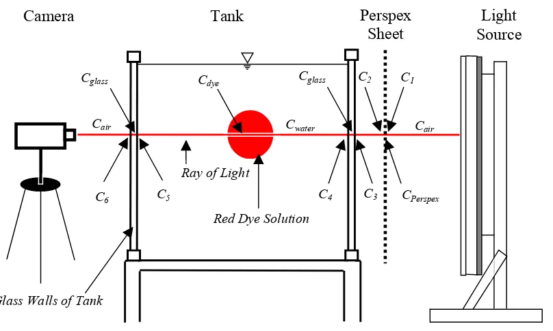
To create a high quality data set two quantitative flow visualizations techniques are used. These are presented in Chapter 3. The first is LIF or Laser Induced Fluorescence. LIF has been used for nearly two decades and has been used to visualize buoyant jets for the past decade. LIF performs well for investigations into the behaviour of flows with two-dimensional trajectories and is used in the present study during the investigation of discharges in a still ambient fluid (in particular the negatively buoyant jet). An alternative flow visualization technique is developed to help with the investigation into the behaviour of three-dimensional trajectory flows. It is referred to as LA or Light Attenuation and is also employed for the two-dimensional trajectory flow experiments. The technique is based on a linear relationship between the increase in concentration of dye in the water and decrease in the intensity of the light passing through it.

(30)

A wide range of LA experiments have been conducted. This is firstly done to verify the visualization technique, secondly to provide additional insight into the behaviour of discharges with two-dimensional trajectories, and finally to investigate the behaviour of discharges with three-dimensional trajectories. In Chapter 5 results for a range of initial discharge configurations are presented and comparisons are made with existing data and model predictions, as well as predictions from the Momentum Model.

A more detailed investigation is carried out into the behaviour of negatively buoyant jets and this is described in Chapter 6. There is a growing interest in the process of desalination to produce drinking water, because of increased uncertainties in water supply associated with unstable weather patterns. Discharges from desalination plants are in the form of negatively buoyant jets (wastewater with a higher density than the receiving ambient). Earlier investigations have primarily focused on a single angle of discharge (60º). The present investigation expands that to a range of angles and includes a comparison with both analytical and numerical model predictions.

Another flow with a two-dimensional trajectory that is investigated in more detail is the non-buoyant oblique discharge in a moving ambient. Both horizontally and vertically released non-buoyant discharges in a moving ambient have been studied in the past and the influence of the ambient on the flow in the strongly advected region was found to be significantly different for the two cases. The attention of the current investigation is focused on the transition angle that defines the distinctly different final forms of flow behaviour. The theoretical and experimental investigations can be found in Chapter 7.

Finally, the results of the experimental investigation into the behaviour of three-dimensional trajectory flows are presented in Chapter 8. As the knowledge of these flows is limited, the main purpose of the study is to observe these flows in general, comment on their behaviour and compare the results with predictions from current models.

(31)

Chapter 2 – Review of Previous Research

2.1 – Introduction

In this chapter an overview is given of relevant research undertaken into the behaviour of buoyant jets released into an unstratified ambient. For over a century research into this topic has been carried out and this has resulted in extensive knowledge about the theory of buoyant jets. The theories developed have formed the basis for several mathematical models and a summary of the models as well as their theoretical background is presented. Experimental investigations have led to considerable quantities of relevant experimental data on buoyant jets. Previous experimental investigations are discussed in this chapter and flow configurations with very limited experimental data are highlighted.

2.2– Problem Formulation of the Buoyant Jet

A (buoyant) jet is generated when relatively fast flowing fluid, from a continuous source, is discharged in a reservoir of relatively slow flowing fluid and the density difference between the two fluids is small. The high velocity gradients at the interface between jet and the ambient fluid make it highly unstable, and cause the jet fluid to rotate. These turbulent vortices entrain the ambient fluid into the jet, causing the mixing processes and the dissipation of the energy from the discharge.

(32)

As the distinct flow regions are the same for buoyant jet flows with two-dimensional and three-dimensional paths, it is assumed that the understanding of the behaviour of the flow, gained from experiments with two-dimensional trajectories, can also be applied to buoyant discharges with three-dimensional trajectories. Models based on this approach are assumed to predict with reasonable accuracy the behaviour of discharges with two-dimensional and three-dimensional paths (Cheung et al. 2000; Jirka 2004).

2.3 - Research History

Buoyant jets have been observed and commented on since the beginning of modern science, for example, they were observed coming out of smokestacks and volcanoes. Jirka (2004) gives an extended overview of the history of research on the buoyant jet. Some key features are given here.

It was not until the beginning of the twentieth century that the first detailed experimental measurements and an analytical explanation were completed on the subject. The investigation was lead by L. Prandtl in the 1920’s; he applied boundary layer theory to the jet flow. Soon it was followed by measurements on the round buoyant jet (Zimm 1921) and the plane non-buoyant jet (Förthmann 1934). These measurements were the basis for the development of the similarity solutions for the spread and the velocity decay of the jet (Görtler 1942; Reichardt 1942; Tollmien 1926). Prandtl’s turbulent mixing length hypothesis was used to relate the shear stresses to the mean flow of the jet and this method was taken a step further to include a pure vertically rising plume by Schmidt (1941). Reichardt (1943) was the first to determine that the cross-sectional properties of the jet could be approximated by Gaussian profiles, forming the foundation of the jet-integral method. The method was further developed into a jet integral model with the results of more detailed experiments carried out on the simple jet (Albertson et al. 1949) and the pure plume (Rouse et al. 1952).

(33)

Turner (1960) and Richards (1963) showed that an internal double vortex pair significantly affected the velocity and scalar distributions when the jet or plume flow was strongly deflected by the ambient current.

2.4 – Previous Experimental Investigations

Over the past six decades many experimental studies have been carried out in the field of buoyant jets. Most of these studies have been carried out in the laboratory. Data from field studies is available, but it was not possible to measure all the major factors influencing the flow behaviour and therefore the data is difficult to interpret. Because of the less-controlled environment outside the laboratory the results were less accurate. Inside the laboratory it is possible to separate the important independent parameters, the initial momentum flux, the buoyancy-generated momentum flux and the ambient momentum flux, from outside influences and from each other. This enables the researcher to carefully determine the influence of each of the factors on the flow. The laboratory studies differed in the use of measurement techniques, aims and types of flow. Because of the increase in the technology available to researchers over time, the studies have become more detailed; the flow measurement techniques more accurate and more complex flow configurations have been monitored. Data from experimental investigations has been used for verification of models as well as determination of the empirical parameters in the length-scale and integral models (see section 2.5).

2.4.1 – Flow measurement techniques

An overview of the main techniques used to measure velocity and concentrations in buoyant jets is given below.

(34)

the high local turbulence intensity, caused by the flow around the stationary wires, with the Flying Hot-Wire anemometry (FHW) (Hussein et al. 1994). With the introduction of Particle Image Velocimetry (PIV) (Simoens and Ayrault 1994), velocity measurements were no longer confined to a point, but a planar velocity field could be observed and measured

Concentration measurements were made by Ayoub (1971) using conductivity probes, which were used to determine mean cross-sectional concentration profiles, and a black and white still camera in combination with potassium permanganate dye was used to determine the flow trajectory. For the buoyant jet in a cross-flow experiments a second black and white camera was added to record the trajectory in both the x-y and x-z planes. Papanicolau (1984) investigated the concentration profiles of a buoyant jet in a still ambient using laser-induced fluorescence (LIF), a non-intrusive optical technique, giving both trajectory and instantaneous concentration measurements. Knudsen (1988) added red dye to her experiments and recorded the trajectory using either a photographic or video camera. The trajectory of the centreline was determined by the averaging the two points defining the visible edges of the flow. With the known trajectory, a set of suction probes was inserted into the flow to measure the concentration at a pre-determined location. The upgrade of LIF to Planar Laser-Induced Fluorescence (PLIF) (van Cruyningen et al. 1990) did for the concentration measurements what PIV has done for the velocity measurements. Hereafter Laser Induced Fluorescence and Planar Laser-Induced Fluorescence are both referred to as LIF. However, simpler techniques continue to provide valuable information. For example, Cheung (1991) used hot water, rather than salt water, to create a difference in density between ambient and jet fluid. Rows of thermistor probes or a single thermilinear probe were then used to find the cross-sectional concentration field. The centre of mass of the concentration field defined the trajectory.

Experimental studies have also employed more than one measurement technique to obtain both velocity and concentration data, or to compare results from more than one technique as an internal verification. Examples are Papanicolau (1984) and Chu (1996) using both LDA and LIF, and Wang (2000a) using both PIV and LIF.

2.4.2 – Flow configurations

(35)

incorporated into subsequent chapters where appropriate. Note that x is the Cartesian coordinate in the same direction as the ambient velocity; or in the direction of the horizontal component of the initial velocity for still ambient flow, z is the Cartesian coordinate in the same direction as the vertical component of the initial velocity, and y is the Cartesian coordinate perpendicular to the x-coordinate in the horizontal plane. The angle

φ

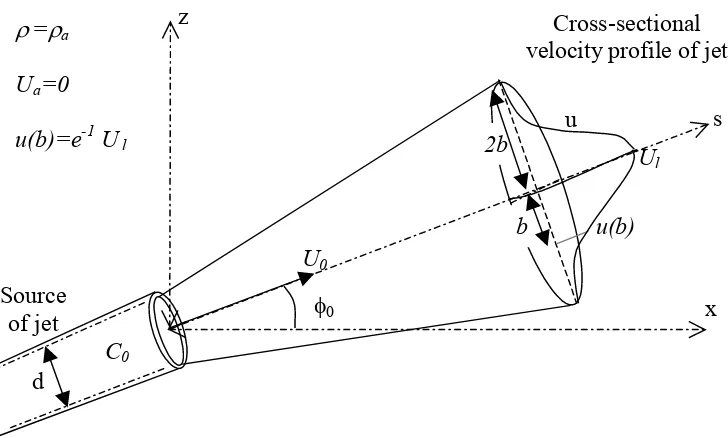
0 is the angle between the excess momentum flux and the ambient momentum flux; or between the excess momentum flux and the x-axis for still ambient flows, and s is the distance from the source along the trajectory of the flow.

2.4.2.1 - Jets

The first experimental investigations were on the behaviour of the simple jet. A simple jet flow has no buoyancy flux, as the density of the fluid in the jet (

ρ

) and the density of the ambient fluid (

ρ

a) are the same, and the ambient environment is stationary (the ambient

velocity (Ua) is zero). The behaviour of the flow is therefore dominated by the initial

momentum flux (M0 =Q0 U0, where U0 is the initial (uniform) velocity of the flow, and Q0 is

the flow rate of the discharge) and is independent of the initial angle of discharge (

φ

0). Investigations by Corrsin (1943), Hinze and van der Hegge Zijnen (1949), Albertson et al (1949), Corrsin and Uberoi (1950), Forstall and GayLord (1954), Sunavala et al. (1957), Ricou and Spalding (1961), Kiser (1963), Rosler and Bankoff (1963), Becker et al. (1967), Wygnanski and Fiedler (1969), Crow and Champagne (1971), Labus and Symons (1972), Birch et al. (1978), Capp (1983), Hussein et al. (1994), Pun (1998), Law and Wang (2000) and others have led to a firm understanding of the spread, velocity and dilution profiles as well as the rate of entrainment of the simple jet. The mean cross-sectional velocity and concentration profiles were both shown to fit the Gaussian shape well. Later experiments involving a simple jet have been carried out as a first step towards more complicated flow configurations or to investigate the instantaneous behaviour, including the turbulent properties of the jet. A schematic representation of a jet flow can be seen in Figure 2.1, including a mean cross-sectional velocity profile at some distance away from the source. The cross-sectional centreline velocity is represented by Ul, the local velocity in the cross-section by u, and the

(36)

initial concentration of an inert pollutant added to the jet fluid, and d is the diameter of the source.

s u

d

x

2b

φ0

ρ

=

ρ

a

Ua=0

u(b)=e-1 U l

b

Ul

U0

u(b)

Source of jet

Cross-sectional velocity profile of jet

of jet

C0

[image:36.595.114.478.111.330.2]

z

Figure 2.1 - Initial conditions and cross-sectional velocity profile for jet experiment

2.4.2.2 – Pure Plumes

(37)

d

z

x

φ0

ρ

<

ρ

a

Ua=0

u(b)=e-1 U l

U0

u

b Ul

u(b)

Source of discharge

Cross-sectional velocity profile of plume

of jet

2b

[image:37.595.165.420.56.321.2]

C0

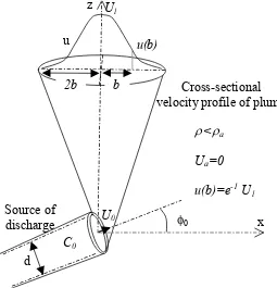
Figure 2.2 - Initial conditions and cross-sectional velocity profile for pure plume

2.4.2.3 – Buoyant Jets

(38)

d

y

x

φ0

ρ

<

ρ

a

Ua=0

u(b)=e-1 U l

Ul

U0

u(b)

Source of jet

Jet-like region of flow z

Ul

u(b)

b 2b

Plume-like region of flow

Jet-to-Plume transition region

of flow

[image:38.595.73.530.64.364.2]

C0

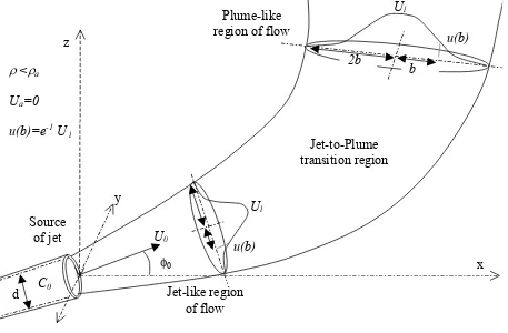
Figure 2.3 - Flow regions of a buoyant jet

Vertically discharged buoyant jets are commonly released such that the initial momentum flux acts in the same direction as the buoyancy-generated momentum flux. Extensive knowledge is available on the behaviour of these vertically discharged buoyant jets because of studies by Rouse et al. (1952), Abraham, (1960), Ricou and Spalding (1961), Abraham (1963), Frankel and Cumming (1965), Anwar (1969), George et al. (1977), Nakagome and Hirata (1977), Papanicolaou and List (1988), Fisher (1995), Pun (1998), Wang and Law (2002) and others.

Changing the source configuration to a horizontal position creates a horizontal buoyant jet. This buoyant jet configuration has been studied by, amongst others, Hanson and Schroder (1968), Anwar (1969), Ayoub (1971), Fan (1967), Hofer and Hutter (1981), Papanicolaou (1984), Papantoniou and List (1989), Davidson (1989), Gaskin and Wood (1993), and Papps (1995).

(39)

initial momentum flux acts in the opposite direction of the buoyancy force. Zeitoun et al. (1972), Roberts and Toms (1987), Roberts et al. (1997) and Cipollina et al. (2005) have studied negatively buoyant jets with an initial discharge angle of -60°. Zeitoun et al. and Cipollina et al. also included initial discharge angles of -30° and -45°. The vertically discharged negatively buoyant jet is commonly referred to as a fountain. Here the flow reaches a maximum height before reversing direction. Turner (1966), Abraham (1967), James et al. (1983), McLellan and Randal (1986), Baines et al. (1990) and Zhang and Baddour (1998) have investigated the vertically discharged negatively buoyant jet.

2.4.2.4 – Advected Jets

(40)

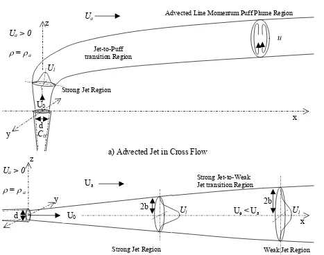
(1998). Advected jets in a counter-flow have been investigated by Yoda and Fielder (1996) and Lam and Chan (2002).

2b d

d

2b U0

Ua > 0

ρ = ρ a

U0

Strong Jet Region

Advected Line Momentum Puff Plume Region

Weak Jet Region

u

StrongJet Region

Ua

a) Advected Jet in Cross Flow

b) Advected Jet in Co-Flow

Ue < Ua

C0

z

y

Ul

Jet-to-Puff transition Region

Ua > 0

ρ = ρ a

Ul Ul

Strong Jet-to-Weak Jet transition Region y

z

[image:40.595.68.535.109.477.2]

x x

Figure 2.4 - Different flow regions of advected jet

2.4.2.5 – Buoyant Discharges in an Ambient Flow

(41)

two-Chapter 2 – Review of Previous Research

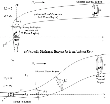
dimensional or a three-dimensional trajectory flow is created. If the initial momentum flux acts in the same plane as the buoyancy-generated and ambient entrained momentum flux, the resulting flow has a two-dimensional trajectory. The focus of past experimental investigations for buoyant discharges in an ambient flow has largely been on 2D trajectory flows, and in particular on either the vertically discharged buoyant jet (Figure 2.5a) or the co-flowing case where the flow is discharged horizontally (Figure 2.5b).

u

d

U0

Ua > 0

ρ < ρ a

U0

(Advected Line Momentum Puff /Plume Region)

StrongJet Region (+ Advected Plume Region)

Ua

a) Vertically Discharged Buoyant Jet in an Ambient Flow

b) Horizontally Discharged Buoyant Jet in an Co-Flow

C0

z

y

Ul

Ua > 0

ρ < ρ a

Ul

y

z

x Advected Thermal Region

u

U0

Advected Plume Region

Strong Jet Region

Ul

Advected Thermal

[image:41.595.88.525.185.596.2]

Region x

Figure 2.5 – Flow regions of buoyant jet in flowing ambient with a 2D-trajectory

(42)

strong jet region, the flow is an advected line momentum puff. After either the plume or puff regions a second flow transition takes place and the flow is then in the advected thermal region where both the buoyancy-generated and the entrained ambient momentum flux dominate the flow. In the weakly advected flow regions (strong jet and plume regions) the deflections due to the ambient current are small. In the strongly advected region (advected line momentum puff and advected thermal regions) the flow is noticeably bent over due to the ambient current and the velocity and concentration profiles resemble a counter-rotating vortex pair. Experimental investigations into this flow configuration have been carried out by Fan (1967), Chu and Goldberg (1974), Wright (1977) and Cheung (1991). Hewett (1971) investigated the vertical heated jet in a cross-flow.

By changing the angle of release of the discharge so that it is in line with the ambient current a buoyant jet in a co-flow is produced (Figure 2.5b). In this situation it is not possible for an advected line momentum puff to form and the presence of buoyancy effectively eliminates the possibility of the formation of a weak jet. Thus only three different flow regions are possible (strong-jet, plume, advected thermal), making their identification relatively simple. Ayoub (1971), Knudsen (1988), Davidson et al (1991) , Wong and Lee (1991) and Gaskin and Wood (1993) have studied the horizontal buoyant jet in a coflow.

Experimental studies into the behaviour of buoyant jets with two-dimensional trajectories in an ambient flow with discharge configurations that differ from the two mentioned above are less common. Knudsen (1988) studied the horizontal buoyant jet in a counter-flow. Chu (1975b) and Anderson et al. (1973) have investigated the behaviour of negatively buoyant jets in a cross-flow. Chu released the initial momentum flux perpendicular to the ambient flow; Anderson et al. released the initial momentum flux at 60° to the cross-flow.

(43)

or velocity profiles of the flow at one or several points, setting up the measuring equipment at the point of interest (perpendicular to the direction of flow). However with none of the trajectory co-ordinates fixed, locating the trajectory and the direction of flow required a separate investigation. The introduction of LIF made it possible to obtain more detailed information at a particular cross-section, but locating the cross-section so that it was perpendicular to the flow direction remained problematic. Determining the trajectory co-ordinates from photographs or video images is difficult because of the changing calibration length-scales, due to the flow not travelling perpendicular to the plane of view. However, the above-mentioned constraints are largely eliminated for areas of the flow that travel predominantly in a single direction, reducing the flow to one with an essentially two-dimensional trajectory (Cheung 1991). Ayoub (1971), Chu (1975a) and Cheung (1991) studied the horizontally discharged buoyant jet in a cross-flow and Wallingford Hydraulic Research Station (1977) the horizontally discharged heated jet in a cross-flow.

Ul

U0

d

Advected Thermal Region Advected Plume Region

Strong Jet Region

Ua > 0

ρ < ρ a

Ua z

x

y

Figure 2.6 – Flow configuration horizontally discharged buoyant jet in a cross-flow

2.4.3 – Missing Experimental Data

(44)

have investigated these flows have largely been limited to trajectory results. These flows are of particular interest because they provide an opportunity to study more closely the nature of transitions between the different strongly advected regions. In the non-buoyant case these regions are the weak-jet and the advected line momentum puff. More generally, currently available models predict oblique discharge behaviour and validation of these predictions with experimental data is desirable.

With the increase in the demand for clean water as well as decreasing costs for the desalination process, desalination plants are becoming an increasingly viable option as a supplementary reliable main water supply for many communities. The effluent from desalination plants has relatively high salinity concentrations. Discharging the effluent into less dense surrounding fluid makes the effluent fall rather than rise. If the ambient motion is relatively small or non-existent the discharge essentially becomes a negatively buoyant jet. Except for the vertical discharge configuration, the negatively buoyant jet has not received a great deal of attention. Past experimental investigators have primarily studied the behaviour of the discharge with a 60° angle, and to a lesser extent the 30° and 45°. The experimental results have focused on the rise height of the flow, the distance from the point of release to the impact point (the point at which the flow returns to the source height), and the dilution at the impact point. Widening the scope of the investigation into the behaviour of the negatively buoyant jets (including a range of discharge angles and determining spread and dilution data along the trajectory of the flow), will increase the knowledge of the mixing characteristics of these flows. This understanding can eventually lead to more effective discharge techniques.

(45)

2.5 - Existing Models

The considerable research activity in this area over the past 50 years has resulted in a number of different models to mathematically describe the trajectory and dilution of buoyant discharges. Over time these models have expanded to incorporate more complex flow configurations. Most models are now able to predict the behaviour of a buoyant jet with a three-dimensional flow trajectory. The different models can generally be split into three different categories, the length-scale models, the integral models, and the models that use a combination of both length-scales and integral techniques.

2.5.1 – Length-Scale Models

The first group of models is based on the length-scale approach (for a more detailed explanation, see Pun (1998)). The first step in this approach is to determine the different flow regions. For buoyant jets in a cross-flow, the different flow regions or limiting cases are the initial, strong jet, weak jet, line momentum puff, advected plume and advected thermal. These flow regions are determined by the relative magnitude of the independent parameters of the flow. The independent parameters are the initial flow rate (Q0), initial excess momentum flux

(Me0), the initial density deficit flux (Q∆0) and the ambient velocity (Ua). Table 2.1 shows the

dominant parameters for each of the different flow regions. U0 represents the initial (uniform)

velocity of the flow at the end of the round source, d the diameter of the source, g the gravitational constant,

ρa

the density of the ambient fluid,

ρ

the density of the jet fluid, and

φ0

the initial discharge angle.

(46)

transition length-scale relationships. These constant are obtained from comparisons with experimental data.

Table 2.1 - Dominant parameters in flow regions

Flow Region Dominant Parameters

Initial Q0

(

=π 4d U2 0

)

Strong Jet Me0

(

=Q0Ue0 =Q0

[

U0 −Ua

]

)

Weak Jet Me0 and Ua

Line Momentum Puff Me0 and Ua

Advected Plume Q_∆₀

(

=Q g₀

(

ρ

_a −

ρ ρ

)

Advected Thermal Q_∆₀ and Ua

Table 2.2 – Transition length-scales for transition between flow regions

Flow Region Transition Transition Length-Scale

Initial – Strong Jet 0

1 2 0 e Q M ∼

Initial – Advected Plume

3 5 0 1 5 0 Q Q_∆ ∼

Initial – Advected Thermal

2 0 0 a Q U Q_∆ ∼

Strong Jet – Weak Jet

1 2 0 0 cos e a M U φ ∼

Strong Jet – Advected Line Momentum Puff

1 2 0 0 sin e a M U φ ∼

Strong Jet – Advected Plume

3 4 0 0 e M Q∆ ∼

Weak Jet – Advected Thermal 0

0 0

cos

e a

M U

Q_∆ φ

∼

Advected Plume – Advected Thermal 0 3 a Q U ∆ ∼

Advected Line Momentum Puff – Advected Thermal 0

0 0

sin

e a

M U

Q_∆ φ

(47)

The second step involves working out relationships that describe flow behaviour within a flow region using dimensional analysis. With the help of the Buckingham Π theorem the trajectory, spread, velocity and dilution can be related to the distance from the source or the virtual source (see Table 2.3). The virtual source of a flow region is the location of the source if the flow was released in that particular flow region. Appropriate constants are introduced that can again be obtained from experimental data.

Table 2.3 – Characteristic relations of flow parameters with distance within flow regions

Flow Region Trajectory Spread Velocity Dilution Strong Jet (vertical discharge) _z _x1 2

∼ ∼z1 ∼ z−1 ∼z1

Weak Jet (horizont

Buoyant jets with two and three dimensional trajectories