Analogue modelling of strike slip surface ruptures: Implications for Greendale Fault mechanics and paleoseismology

_____________________________________________________________________________________

A

NALOGUE MODELLING OF

STRIKE

-

SLIP SURFACE RUPTURES

:

I

MPLICATIONS FOR

G

REENDALE

F

AULT

MECHANICS AND PALEOSEISMOLOGY

B

Y

P

ERI

J

ORDAN

S

ASNETT

A thesis submitted in partial fulfilment of the requirements for the

degree of Master in Science of Geology at the University of Canterbury

ii

A

Analogue modelling of strike-slip faulting provides insight into the development and

behaviour of surface ruptures with accumulated slip, with relevance for understanding how

information recorded in paleoseismic trenches relates to the earthquake behaviour of active

faults. Patterns of surface deformation were investigated in analogue experiments using cohesive

and non-cohesive granular materials above planar strike-slip basement faults. Surface

deformation during the experiments was monitored by 3D PIV (particle image velocimetry) and

2D time lapse photography. Analysis focused on fault zone morphology and development, as

well as the relationship of the models to surface deformation observed at the Greendale Fault that

resulted from the 2010 Darfield earthquake.

Complex rupture patterns with similar characteristics to the Greendale Fault (e.g. en

echelon fractures, Riedel shears, pop-up structures, etc.) can be generated by a simple fault plane

of uniform dip, slip, and frictional properties. The specific structures and the style of their

development are determined by the properties of the overburden and the nature of the material

surface. The width of the zone of distributed deformation correlates closely with sediment

thickness, while the width of discrete fracturing is controlled by the material properties as well as

the thickness of the overburden. The overall deformation zone width increases with the growth

of initial, oblique fractures and subsequently narrows with time as strain localizes onto discrete

fractures parallel to the underlying basement fault.

Mapping the evolution of fracture patterns with progressive strain reveals that Riedel

shears, striking at 90-120° (underlying fault strike = 90°) are more frequently reactivated during

iii

This will help identify suitable locations for paleoseismic trenches and interpret trench records

on the Greendale Fault and other active, strike-slip faults in analogous geologic settings. These

results also highlight the tendency of trenching studies on faults of this type to underestimate the

number and displacement of previous ruptures, which potentially leads to an underestimate of the

iv

A

So many people have combined to help this thesis come together, and first and foremost

among them are my supervisors. Mark, I’m so glad you agreed to take me on as a student and

make this opportunity possible. You’ve made a lot of time for me at a point when you didn’t

have much to spare, and I appreciate it. Sandy and David, you both looked after me so well in

Australia. Having minimal experience with analogue modelling, I was reliant on you to figure

out how to make my grand ideas into an actual model, and you totally came through. Pilar, you

are the best brainstorming partner ever. The days you spent with me talking through my thesis

and outlining the final version have made these few months of writing infinitely easier, and I am

very grateful. Also, thanks for teaching me to make mole!

The Fulbright US Student Program made it possible for me to come back to New Zealand

for postgraduate study. Fulbright New Zealand, specifically, did a wonderful job welcoming me

and the other grantees to the country and supporting us during our time here. I also feel very

lucky to have such awesome fellow Fulbrighters—you guys are the best, and I can’t wait to see

you all back in the States.

I’m also grateful to the University of Canterbury geology community that adopted me so

effortlessly. Darren, Sam, and Anekant: Frontiers was the perfect re-introduction to New

Zealand, both geologically and otherwise. Thanks to the staff as well—you have all been

inexplicably eager to help me solve any problem, from the initial last minute decision to do a

Masters, to constant requests for plane tickets a week in advance (sorry!). To the other UC

v

evenings (or afternoons…) at the Shilling Club. Also, a big shout out goes to the UC wiffleball

team—let me know when it’s time to organize an international tour.

Last but certainly not least, thanks to my friends, flatmates, and family. Past and present

Peer Streeters—and honorary ones, you know who you are—there’s no way I would have gotten

this far without your constant, loving harassment. Kat, Kate, Kate, Courtney, and Louise, thanks

for all the fun times, great chats, and many (many) wines. Mom and Dad—you guys get all the

credit for gently suggesting I come back to New Zealand, and even more credit for actually

letting me go abroad for so long. I’m so grateful for your support and encouragement, and your

vi

T

C

A

A

T

C

L

F

L

T

1.

I

R

C

K

1.1 Introduction ...1

1.2 Regional Geology ...3

1.2.1 Regional Tectonic Context ...3

1.2.2 Greendale Fault and Canterbury Plains Stratigraphy ...5

1.3 Previous Studies of Strike-Slip Deformation ...9

1.3.1 Field Observations ...9

1.3.2 Analogue Modelling Studies ...14

1.4 Research Questions and Objectives ...16

2.

M

2.1 Experimental Setup ...18

2.2 PIV Setup ...19

2.3 Materials Tested ...19

2.4 Material Properties ...25

2.5 Scaling ...30

2.6 Experiments ...32

2.7 Greendale Fault Datasets ...34

2.8 Analysis of Analogue Models and Greendale Fault Data...36

3.

F

Z

D

C

S

M

A

E

vii

3.2 DATA AND RESULTS ...39

3.2.1 Experimental Results ...39

3.2.1.1TALC and TALC_PIV ...39

3.2.1.2TALC_SED ...46

3.2.1.3TALC_ER ...51

3.2.1.4TALC_SAND and TALC_SAND_PIV ...56

3.2.1.5SAND_PIV ...64

3.2.1.6General Summary ...68

3.2.2 Greendale Fault Trace ...71

3.2.2.1Stepovers ...76

3.3 DISCUSSION ...78

3.3.1 Comparisons with the Greendale Fault ...78

3.3.1.1 Qualitative Comparisons ...78

3.3.1.2 Quantitative Comparisons ...81

3.3.1.3 Deformation Zone Width...88

3.3.1.4 Scaling...94

3.3.2 Effects of Interseismic Sedimentation and Erosion ...96

3.3.2.1Experimental Data ...96

3.3.2.2Application to Active Faults ...98

3.3.3 Stepovers ...101

3.4 CONCLUSION ...104

4.

A

O

A

M

T

P

4.1 Introduction ...106

4.2 Data and Results ...107

4.3 Discussion...113

4.3.1 Reactivated Structures: Analogue and Field Examples ...113

4.3.2 Effects of Surface Cementation ...118

4.3.3 Relationship of Rupture Morphology to Fault Zone Development ...119

4.4.4 Implications for Paleoseismology ...119

4.4 Conclusion ...123

viii

R

A

Appendix A: Macro Stepover Experiments ...135

Appendix B: Shear Wagon Data ...138

Appendix C: Analogue Model Photographs (also see supplemental discs) ...143

ix

L

F

Figure 1.1. Map showing Canterbury Plains with Greendale Fault trace and location of

aerial photos referred to in text ...1

Figure 1.2. Map showing New Zealand’s regional tectonic setting ...4

Figure 1.3. Annotated aerial photos of Greendale Fault rupture ...6

Figure 1.4. Model of Greendale Fault subsurface geometry (Holden et al., 2011) ...7

Figure 1.5. Model of Greendale Fault subsurface geometry (Elliott et al., 2012) ...8

Figure 1.6. “Riedel within Riedel” patterns at the Greendale Fault ...10

Figure 1.7. Schematic “Riedel within Riedel” pattern ...11

Figure 1.8. Block diagram showing 3D helicoidal geometry of Riedel shears ...12

Figure 1.9. “Riedel within Riedel” patterns from the Dasht-e-Bayaz earthquake rupture and from an analogue model...13

Figure 1.10. Strain ellipsoid for right lateral simple shear ...14

Figure 2.1. Photograph of experimental setup ...18

Figure 2.2. Photograph of SAND experiment ...20

Figure 2.3. Photograph of preliminary test ...21

Figure 2.4. Photograph of preliminary test ...22

Figure 2.5. Photograph of preliminary test ...23

Figure 2.6. Photograph of preliminary test ...24

Figure 2.7. Example plot of shear wagon data for fine sand ...25

Figure 2.8. Example plot of shear wagon data for talc ...26

Figure 2.9. Plot of σXY vs. σ for fine sand at peak and stable strength ...27

Figure 2.10. Plot of σXY vs. σ for talc powder at the point of yielding, and after 10, 20, and 30 mm displacement of the shear wagon ...28

Figure 2.11. Schematic cross sections of experimental setup ...33

Figure 2.12. Examples of Greendale Fault hillshade, aspect, and slope datasets ...35

x

Figure 3.2. Distribution of fracture azimuths in TALC at progressive strain intervals ...41

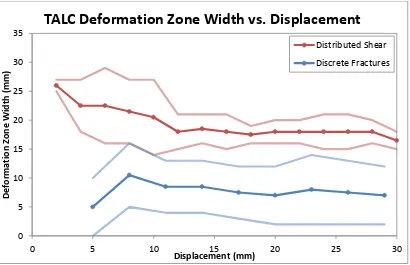
Figure 3.3. TALC fracture length plotted versus fracture azimuth, cumulative and individual ... 41-42 Figure 3.4. Plot showing development of TALC deformation zone widths (both discrete fracturing and distributed shear) with continuing displacement ...43

Figure 3.5. TALC_PIV data showing shear strain distribution ... 44-46 Figure 3.6. TALC_SED images at successive strain increments with corresponding fracture maps ...48

Figure 3.7. Distribution of fracture azimuths in TALC_SED at progressive strain intervals ...49

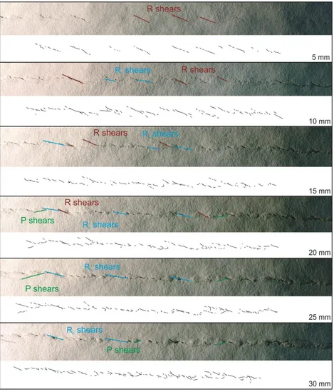
Figure 3.8. TALC_SED fracture length versus azimuth, cumulative and individual ... 49-50 Figure 3.9. TALC_ER images at successive strain increments with corresponding fracture maps ...52

Figure 3.10. Distribution of azimuths in TALC_ER by displacement increment ...53

Figure 3.11. TALC_ER fracture length versus azimuth, cumulative and individual ... 54-55 Figure 3.12. Development of TALC_ER discrete fracture zone width with continuing displacement ...56

Figure 3.13. TALC_SAND images at successive strain increments with corresponding fracture maps ...57

Figure 3.14. Distribution of fracture azimuths in TALC_SAND with ongoing strain ...58

Figure 3.15. TALC_SAND fracture length vs. azimuth, cumulative and individual ... 59-60 Figure 3.16. Plot showing development of TALC_SAND deformation zone widths with continuing displacement ...61

Figure 3.17. TALC_SAND_PIV data, showing shear strain distribution ... 62-64 Figure 3.18. Plot showing development of SAND_PIV deformation zone widths with continuing displacement ...65

Figure 3.19. SAND_PIV data, showing shear strain distribution ... 66-68 Figure 3.20. Schematic representation of fault zone behaviour with increasing displacement ...69

Figure 3.21. Mean azimuth for all experiments by displacement increment ...70

Figure 3.22. Mean length for all experiments by displacement increment ...70

Figure 3.23. Scaled function of length and azimuth for all experiments ...71

xi

Figure 3.25. Annotated aerial photos of the Greendale Fault trace ...73

Figure 3.26. Greendale Fault fracture azimuth distribution ...74

Figure 3.27. Greendale Fault fracture length versus azimuth ...74

Figure 3.28. Greendale Fault aerial photos with azimuth distributions ...75

Figure 3.29. Schematic of Greendale Fault stepover measurements ...76

Figure 3.30. Plot of stepover width versus average bounding segment length...77

Figure 3.31. Comparison of central Greendale Fault LiDAR data with TALC_ER at 15 mm displacement ...78

Figure 3.32. Comparison of TALC_SAND with aerial photo of central Greendale Fault surface trace ...79

Figure 3.33. Length vs. azimuth comparison for TALC, TALC_SAND, TALC_SED, TALC_ER, and the Greendale Fault ...82

Figure 3.34. Length vs. azimuth of model data at 10 mm displacement and Greendale Fault data ...84

Figure 3.35. Length vs. azimuth of model data at 20 mm displacement with Greendale Fault data ...84

Figure 3.36. Length vs. azimuth of model data at 30 mm displacement with Greendale Fault data ...85

Figure 3.37. TALC_SED and TALC_ER at 15 mm displacement compared with Greendale Fault data ...85

Figure 3.38. Relative frequency of fracture azimuths in Greendale Fault data as compared with model data ...86

Figure 3.39. Azimuth distribution of Greendale Fault data compared with TALC_ER data ...87

Figure 3.40. Mean width of distributed shear vs. overburden thickness for TALC, SAND, and TALC_SAND at different strain increments ...89

Figure 3.41. Mean width of discrete fracturing vs. overburden thickness for TALC, SAND, and TALC_SAND at different strain increments ...89

Figure 3.42. Width of distributed shearing zone with ongoing displacement for TALC, SAND, and TALC_SAND...90

xii

Figure 3.44. Discrete fracture zone width as a percentage of the distributed shear zone width,

with continuing displacement ...92

Figure 3.45. Schematic representations of model deformation in cross section ...94

Figure 3.46. Comparison of fracture length vs. azimuth for TALC, TALC_ER, and TALC_SED...97

Figure 3.47. “Riedel within Riedel” patterns in TALC_ER and TALC_SED ...102

Figure 4.1. Active deformation traced at 5 mm intervals ...107

Figure 4.2. Active structures superimposed upon one another, highlighting structures being repeatedly reactivated ...108

Figure 4.3. Map of reactivated structures only ...108

Figure 4.4. Length vs. azimuth of reactivated fracture segments ...109

Figure 4.5. TALC_ER length versus azimuth for all fractures ...110

Figure 4.6. Schematic trenches placed along the TALC_ER model fault zone ...111

Figure 4.7. Terrestrial laser scan image overlaying LiDAR image of the Greendale Fault rupture at Highfield Road ...114

Figure 4.8. Schematic drawing showing the distribution of offset through multiple earthquakes on structures in the Highfield Road trench across the Greendale Fault ...115

Figure 4.9. TALC_ER deformation at only 15 mm and 30 mm intervals ...116

Figure 4.10. Same schematic trench locations as Figure 4.6, with only 15 mm and 30 mm structures ...116

Figure 4.11. Annotated aerial photograph of Greendale Fault rupture segment ...121

Figure A.1. Schematic showing experimental setup for stepover experiments ...135

Figure A.2. STEP1.5 fracture maps at successive displacement intervals ...136

Figure A.3. STEP3 fracture maps at successive displacement intervals ...137

Figure B.1. Shear wagon data for fine sand (2 cm) ...138

Figure B.2. Shear wagon data for fine sand (4 cm) ...138

Figure B.3. Shear wagon data for fine sand (6 cm) ...139

Figure B.4. Shear wagon data for fine sand (8 cm) ...139

xiii

Figure B.6. Shear wagon data for talc (2 cm) ...140

Figure B.7. Shear wagon data for fine sand (4 cm) ...141

Figure B.8. Shear wagon data for fine sand (6 cm) ...141

Figure B.9. Shear wagon data for fine sand (10 cm) ...142

xiv

L

T

Table 2.1. Values describing internal friction measured in shear wagon tests ...28

Table 2.2. Scalable parameters for model and natural systems ...31

Table 2.3. Experiment numbers, descriptions, and recording methods ...32

Table 3.1. TALC_SAND scaling ...95

Table 3.2. TALC, TALC_ER, TALC_SED scaling ...95

1

1.

I

R

C

K

1.1 Introduction

Paleoseismic trenching studies are an important part of earthquake hazard analysis,

because they make it possible to establish the rupture history of active faults, calculate slip rates,

and estimate recurrence intervals, parameters which are used to assess the seismic hazard of a

region. The principle of trenching is based on a theoretical model in which a fault’s surface

expression is confined to one or a few main traces, and the trench is placed across a segment that

has ruptured in all or nearly all previous ruptures (e.g. Sieh and Jahns, 1984; Yetton, 1998).

Many fast slipping, mature faults are likely to rupture in this manner, on confined fault traces

(e.g. the San Andreas fault, Sieh et al., 1989; the Wellington Fault, Little et al., 2010; and the

Denali fault, Haeussler et al., 2004), but slower-moving faults with longer recurrence intervals

may result in complex rupture patterns that are more complicated to interpret (e.g. the Darfield

earthquake, Quigley et al., 2012; the El Asman earthquake, Philip and Meghraoui, 1983; the

Dasht-e-Bayaz earthquake, Tchalenko and Ambraseys, 1970).

On faults that generate distributed surface deformation (e.g. the Dasht-e-Bayaz Fault,

Tchalenko and Ambraseys, 1970; the Greendale Fault, Quigley et al., 2010), it is much more

challenging to identify a “main fault trace” on which paleoseismic studies should be focused. If

some paleoruptures are not identified, or not even visible in trenches, or if only a fraction of the

offset is measurable, the results of these studies could lead to significant underestimates of future

earthquake hazard. A deeper understanding of the behaviour and development of strike-slip

2

Analogue modelling has frequently been used to study strike-slip faulting, specifically the

development of deformational features (e.g. Riedel, 1929; Tchalenko, 1970; Naylor et al., 1986;

Schreurs, 1994; Richard et al., 1995), or basin formation and potential resource trapping

structures (e.g. Wilcox et al., 1973; McClay and Dooley, 1995; Rahe et al., 1998), but the use of

analogue models to inform paleoseismic interpretations of active faults has not been previously

considered to the best of my knowledge.

The Greendale Fault rupture extends for ~30 km across the Quaternary surface of the

Canterbury Plains, with a deformation zone that ranges from 30-300 m wide consisting of both

concentrated fracturing and distributed shear (Figure 1.1; see section 1.2.2 for details; Quigley et

3

al., 2012). The diffuse character of this deformation—where even the most focused rupture area

is distributed over tens of meters and hundreds of small-scale fractures—has complicated efforts

to situate paleoseismic trenches in ideal locations to study the earthquake history of the fault.

Even with an unusually detailed rupture map to guide paleoseismic studies, there is no guarantee

that recent high-displacement structures are the same ones that have been previously active or

that will be in the future.

This investigation uses simple analogue experiments to gain further insight into the

behaviour of strike-slip faults rupturing through granular, cohesive materials. The models were

adjusted to test the effect on surface morphology of parameters such as sediment thickness,

sediment type, cohesiveness, and interseismic sedimentation and erosion, and the resulting

surface fractures were mapped and analysed at various strain increments.

This information was used to address questions about the Greendale Fault rupture relating

to the appearance of surface deformation and its relationship to past events, and how this

knowledge can help constrain paleoseismic studies. Specifically, why was the deformation zone

so wide (up to 300 m; Van Dissen et al., 2011) and what controls the relationship between

distributed deformation and discrete fracturing? Is this type of surface deformation a function of

near-surface material properties or fault geometry at depth? What do the fracture patterns reveal

about the fault’s development and slip history? In such a complex network of fractures, how can

one identify the fractures that persist through repeated ruptures and therefore provide the best

targets for paleoseismic studies?

1.2 Regional geology

4

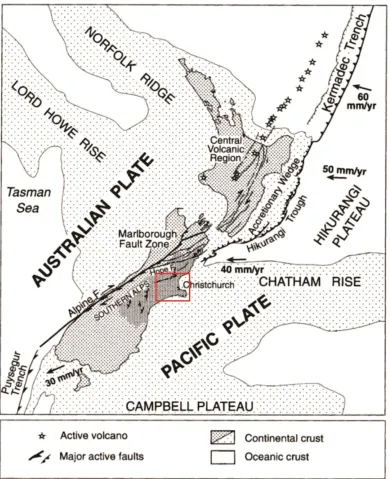
The South Island of New Zealand straddles the boundary between the Pacific and

Australian plates, which converge obliquely at 39-50 mm/yr (Demets et al., 2010).

Approximately 70-75% of plate boundary motion is taken up along the Alpine Fault, a

right-lateral transpressive fault that bisects the South Island (Figure 1.2; Norris and Cooper, 2001).

5

The remainder of this deformation is distributed eastward along faults within the Southern Alps

and beneath the Canterbury Plains (Pettinga et al., 2001). In the Canterbury region, many of

these faults are east-west oriented faults that initiated as steeply-dipping normal faults during late

Cretaceous to Eocene extension (Ghisetti and Sibson, 2012). These faults are reactivated as

dextral strike-slip within the contemporary stress field with maximum compressive stress (σ1)

oriented at 115±5° (Sibson et al., 2011; 2012). Examples include the Greendale Fault, the

Springbank Fault, and the Ashley Fault (Jongens et al., 2012).

1.2.2 Greendale Fault and Canterbury Plains Stratigraphy

The Greendale Fault ruptured in the September 4, 2010 Darfield earthquake, with its

epicentre located ~44km west of Christchurch, New Zealand. It was followed by an energetic

aftershock sequence, including three damaging events of MW > 6.0. However, the Darfield

earthquake was the only one that generated a surface rupture. The flat, agricultural landscape of

the Canterbury Plains, and the abundance of linear markers such as roads, fences, and shelter

belts, facilitated detailed mapping of the rupture, producing a dataset that provides opportunities

to study earthquake-induced surface deformation in high resolution (e.g. Quigley et al. 2012;

Duffy et al., 2013).

The Greendale Fault rupture trace was 29.5±0.5 km in length, with an average right

lateral displacement of 2.5±0.1 m (maximum 5.2±0.2 m) and vertical displacement generally less

than 0.75 m (maximum 1.45±0.2) (Quigley et al., 2012). The surface rupture is made up of two

main segments (eastern and central) that generally strike east-west and a western segment that

strikes northwest (Figure 1.1). The fault zone consists of a wide zone of deformation (30-300 m)

6

structures, as well as distributed shearing (Van Dissen et al, 2011; Quigley et al., 2012). Each of

those en echelon segments consists of a complex pattern of synthetic and antithetic Riedel

shears, tension fractures, and other subsidiary structures (Figure 1.3).

Figure 1.3. Aerial photos of Greendale Fault surface trace: 1120 (A) and 1151 (B), see Figure 1.1 for locations. Fractures are mapped in purple, with R shears highlighted in yellow, R’ shears in red, tension fractures in white, and small thrust structures in blue. (Images courtesy of Mark Quigley.) Arrow indicates north.

The Darfield earthquake is thought to have been the product of near-simultaneous motion

on multiple faults, in addition to the Greendale Fault surface rupture. The initial event occurred

on the Charing Cross fault, a steeply southeast-dipping, blind reverse fault, which triggered the

7

notably one to the southwest of the Greendale fault trace (Gledhill et al., 2011). GPS and InSAR

inversion data suggest motion on a blind reverse fault near the major stepover in the Greendale

fault as well (Figures 1.4, 1.5 (next page); Holden et al., 2011).

Figure 1.4. Model of Greendale Fault subsurface geometry by Holden et al. (2011). Note the presence of blind thrust faults, in addition to the main Greendale Fault plane.

The fault cuts across the Canterbury Plains, which consist of alluvial gravels of late

Pleistocene age (Forsyth et al., 2008). Only the surface and upper few meters of the stratigraphy

beneath the fault have been directly observed, which are made up of fluvial gravels with loess

caps in places. These gravels are moderately indurated to a visible depth of 7 m, as observed in a

quarry on Grange Road, >200 m from the central Greendale Fault. This level of induration is

likely due to weak cementing by pedogenic silica. The Leeston-1 petroleum exploration well

from 1969 is ~10 km south of the central-eastern part of the fault, and it provides the best

estimate of the lower stratigraphy of the Canterbury Plains gravels. The well log shows ~400

8

Figure 1.5. Model of Greendale Fault subsurface geometry by Elliott et al. (2012). These authors model the Greendale Fault as separate segments with variable strikes and dips. Note the presence of additional blind thrust faults that are not modelled by Holden et al. (2011). Fault planes shown near Christchurch city are from the February 22, 2011 earthquake and were not involved in the initial 2010 Greendale Fault rupture.

some marine input toward the bottom of the section (Wood et al., 1989). Beneath this is ~750

meters of more competent rock, including Miocene (Lyttelton Group) and Eocene (View Hill)

volcanics, Cretaceous to Paleocene sedimentary rocks, and the Torlesse basement (Andrews et

al., 1987). However, this stratigraphic section is based on a single well log, so it is not

9

estimate for the depth to basement rock in the central Canterbury Plains of ~750±250 m, which is

in general agreement with the Leeston-1 well log.

1.3 Previous Studies of Strike-Slip Deformation

1.3.1 Field Observations

Strike-slip fault ruptures have been frequently recognized and mapped around the world,

and the geometry and displacements they display at the surface are dependent upon factors like

the material properties of the rocks or sediments that the fault ruptures through, the thickness of

the cover sequence, the topography at the surface, and the maturity of the fault zone, including

frictional properties and fluid pressure of fault rocks, and fracture geometry.

This study specifically focuses on strike-slip ruptures that are expressed in young cover

sequences, which tend to share some common features, particularly en echelon fractures, Riedel

shears, and other associated structures. These classic shear deformation patterns have also been

described in analogue modelling experiments (see section 1.3.2).

Similar experiments have found that the width (perpendicular to fault strike) of the

surface deformation zone is proportional to the thickness of the cover sequence (Naylor et al.,

1986; Atmaoui et al., 2005). The 2001 Kunlun earthquake provides a field example of this

principle because it ruptures through exposed basement rock as well as thick alluvial cover

sequences at different points along strike. In the alluvial deposits, a wide (up to 500 m) shear

zone with frequent R shears was observed, while in the basement rocks, the fault zone was much

narrower (5-50 m wide) and less complex, as predicted by analogue experiments (Lin and

Nishikawa, 2011). Again, this refers only to the zone of discrete fracturing; the zone of broader

10

Strike-slip fault traces tend to manifest as several interacting en echelon segments

connected by stepovers, which can occur on scales from a few meters to a few kilometers

(Wesnousky, 2008). Depending on the geometry of the stepover, related tensile or compressional

stresses in the region between the two fault segments can cause the development of pop-up

structures or pull-apart basins. The Greendale Fault rupture is dominated by left-stepping en

echelon segments with pop-up structures in the restraining stepover areas. These stepovers are

observed on multiple scales, both larger structures between major, ≥400 m segments of the fault,

and smaller structures between ≤200 m fracture zones (Figure 1.6). This “Riedel within Riedel”

pattern (sometimes called a double en echelon pattern) was first observed by Tchalenko (1970)

11

in analogue studies, and has since been frequently noted in strike-slip faulting environments with

a cover sequence above bedrock (e.g. Bjarnason et al., 1993; Clifton and Einarsson, 2005; Carne

and Little, 2012; see Figure 1.7 for a schematic representation). It is not always clear in the field

how different stepover segments relate to one another at depth, whether they are separate

segments (e.g. Elliott et al., 2012; Figure 1.5) or whether they branch from a single fault at depth

(e.g. Carne and Little, 2012; Figure 1.8).

Figure 1.7. Model fault zone showing schematic “Riedel within Riedel” geometry. The blue fractures are classic Riedel shears oriented at 15° clockwise from the principal slip zone (PSZ), while the red structures are equivalent shears made up of an en echelon array of smaller shears oriented at 30° to the PSZ (15° clockwise from the larger scale, blue Riedel shear). Fractures at both these scales can be present simultaneously.

Shear deformation features are rarely as well-expressed in the field as they are in

experiments, but the Greendale Fault is one of few historic ruptures that has generated en

echelon structures and R and R’ patterns in such complexity and so extensively along the rupture

length (Figure 1.3). Its 30-300 m wide deformation zone is also unusual. These characteristics

are partially due to the fault trace’s location in a flat, agricultural landscape with linear markers

12

Figure 1.8. Block diagram showing three dimensional helicoidal geometry of Riedel shears that branch from a single, linear basement fault. (After Richard et al., 1995.)

complexity is also likely related to the material properties of the near-surface gravels or the

circumstances of the fault rupture itself.

The Dasht-e-Bayaz rupture in Iran is relatively similar to the Greendale Fault in terms of

the morphology of the fault trace and the types of structures it displays, particularly R and R’

shears, P shears, and stepovers in a zone of dense fracturing (Tchalenko and Ambraseys, 1970;

Figure 1.9). However, the overall complexity and the diversity of structures seen at Darfield and

in Iran (R, R’, P, etc.) is not always present in other historic ruptures, although similar patterns

have been observed in geomorphic studies of prehistoric deformation (e.g. Keller et al., 1982;

13

Figure 1.9. "Riedel within Riedel" patterns, as seen in A) a field example from the Dasht-e Bayaz earthquake and B) an analogue model of Morgenstern and Tchalenko (1967). Arrows show sense of motion and larger fault trend (Tchalenko, 1970).

Several recent events (e.g. 2003 Bam, Iran earthquake, Hessami et al., 2005; 1990

Rudbar, Iran earthquake, Berberian and Walker, 2010; 2010 El Mayor-Cucapah earthquake,

Oskin et al., 2012; 2010 Yushu earthquake, Li et al., 2012) have much narrower and simpler

shear zones, which are often confined to a single or a few main strands; en echelon fractures are

observed sporadically, but the levels of complexity do not approach that of the Greendale Fault,

even on faults in similar geological environments. It should also be noted that in these cases,

only discrete surface fracturing was measurable, as previously linear markers were not present to

record more subtle distributed deformation. These ruptures occurred in Quaternary sequences

over bedrock, as did the Greendale and Dasht-e-Bayaz ruptures, so it is possible that controls on

fault morphology in these cases are related to surficial factors, such as the material properties of

the Quaternary deposits or the local topography, although fault maturity and other factors

14

1.3.2 Analogue Modelling Studies

The pattern of en echelon fractures in clay slabs undergoing simple shear deformation

was first observed and described by Cloos (1928) and Riedel (1929). These oblique shear

fractures include synthetic “Riedel shears” (R shears) that form at acute angles (90° + φ/2, where

φ is the angle of internal friction and the underlying fault plane strikes at 90°, measured from

north at 0°) to the principal slip zone (PSZ) and antithetic R’ shears that form at angles more

oblique to the PSZ (180° – φ/2; see Figure 1.10). Depending on the materials, tensile cracks (T

fractures) can form parallel to the direction of shortening (σ1, which typically is 45° from the

PSZ), opening in the extension direction (σ3). P shears can also form at a mirror image to R

shears (90° – φ/2), and Y shears are parallel to the underlying fault plane (Figure 1.10).

Figure 1.10. Strain ellipsoid for right lateral simple shear, showing the orientations of maximum compressive stress (σ1) and extension direction (σ3), and the resulting expected angles for synthetic and

15

It is important to note that these fracture orientations are calculated using the Coulomb

fracture criterion, which is based on the frictional properties of the material being deformed. This

gives only one set of orientations for a given material, regardless of its thickness, initial stress

state, the stage of deformation, etc., all of which can result in deviations from the angles

described in Figure 1.10 (e.g. Dresen, 1991; Ueta et al., 2000). A particularly important factor in

these experiments is the three dimensional, helicoidal geometry that Riedel shears develop in

unconsolidated sediments—the thicker the overburden is, the more space there is for the Riedel

shear plane to rotate away from the underlying fault zone, generating fractures that are more

oblique to the PSZ and a wider overall deformation zone (Ueta et al., 2000; Figure 1.8). These

additional controls on the formation of Riedel shears and other fractures can account for a large

amount of variation from the orientations expected based on frictional properties.

Many authors have studied the role that Riedel shears play in the initiation of fault zones

and their development into continuous, throughgoing faults (e.g. Naylor et al., 1986; Schreurs,

1994; Richard et al., 1995). In these analogue experiments on previously undeformed materials,

en echelon sets of R shears generally form first, relatively soon after initial displacement on the

fault at depth. Depending on the specific properties of the model, these can be followed by R’

shears, splay faults, P shears, and other structures that link the initial R shears together into a

single anastomosing fault zone.

The particular conditions of the shear zone are especially important for the formation of

R versus R’ shears. Antithetic R’ shears are much more common when materials are deformed

by a zone of distributed shear, where they sometimes become the dominant structures (e.g.

Hoeppener et al., 1969; Freund, 1974; Schreurs, 1994; An and Sammis, 1996). They are much

16

Richard et al., 1995; Dauteuil and Mart, 1998) or accumulate very little displacement compared

to other structures (e.g. Wilcox et al., 1973; Naylor et al., 1986).

As mentioned previously, analogue modelling studies have shown that for a given stress

state and set of material properties, the width of a fault rupture’s surface deformation zone is

directly related to the total overburden thickness (Naylor et al., 1986; Atmaoui et al., 2005). If

one considers the subsurface branching geometry of Riedel shears, it is clear that if all other

factors are the same, the deeper the “branching point” of the structures, the wider the zone of

deformation will be when they reach the surface (Figure 1.8). To the best of my knowledge, only

a few other analogue modelling studies have focused on the development of surface deformation

zone width with progressive strain (e.g. Atamoui et al., 2005; Schrank et al., 2008).

Analogue modelling of pop-up structures, found at compressional stepovers (i.e. a left

step on a right-lateral fault) has demonstrated that their morphology is mainly controlled by a

few geometric variables: the degree of overlap of the fault segments, the width of the stepover

with respect to the overall fault displacement, and the thickness of the overlying sediments

(McClay and Bonora, 2001). Pull-apart basins are the analogous structure at releasing stepovers.

They demonstrate similar geometric controls, and are often characterized by a cross-basin fault

zone connecting the two fault segments (McClay and Dooley, 1995). Additionally, Schrank and

Cruden (2010) found that dilational effects alone can result in positive and negative topography

changes, depending on the initial compaction of the material.

1.4 Research Questions and Objectives

Existing literature shows how analogue modelling can be of use in understanding the

17

investigate strike-slip faulting in granular materials, in order to better understand the controls on

surface rupture morphology and how it develops with continuing fault displacement. These

findings can then be used to inform how the earthquake history of faults is studied.

In particular, I want to understand whether complex surface deformation is controlled by

the conditions of the fault at depth (i.e. complex fault geometry, rupture dynamics, etc.) or

whether the properties of the overburden and ground surface are more a more important factor.

Similarly, what factors influence the characteristics and width of surface deformation, in terms of

both distributed shear strain and discrete fracturing? I also wanted to explore how fractures form

and propagate in cohesive granular materials.

The goal of this study is to provide insights on the mechanics of the central Greendale

Fault rupture using simple analogue experiments in which the material properties of the

overburden and the finite shear strain are varied. The results of these models can be used to help

understand how faults develop through time, and how earthquake rupture morphology will

change through multiple events. Chapter 4 applies this knowledge to constrain the best locations

for paleoseismic trenches on these types of faults and better interpret the structures exposed in

them. Likewise, the results can help identify structures or phenomena that may be misinterpreted

in trenching studies, which would lead to over- or underestimates of earthquake activity on a

18

2.

M

2.1 Experimental Setup

Analogue experiments were carried out on a shear table that was divided so that one side

could be offset right laterally relative to the other by an electronic actuator at a minimum rate of

1 mm/second. The table was 1 meter long (parallel to the basal velocity discontinuity) and ~40

cm wide. The experiments reported here used roughly half the available area of the shear table

(Figure 2.1). This setup models a planar, vertical strike-slip basement fault at depth, above which

various materials were layered to represent Quaternary cover sediments. The experiments were

recorded with high-resolution time lapse photography and a Particle Imaging Velocimetry (PIV)

system.

19

2.2 PIV setup

PIV is an electro-optical technique that was originally developed for measuring fluid

flow, but has since been adapted for measuring the surface deformation of analogue models (e.g.

Adam et al., 2005; Boutelier et al., 2008; Schrank et al., 2008; Schrank and Cruden, 2010). Two

inclined cameras are set up to record the movement of particles on the surface of the model.

Application of optical cross-correlation algorithms to the resulting images allows the system to

calculate measurements of the instantaneous and cumulative distribution of 2D displacements,

velocity fields, pure and shear strains and strain rates, and 3D topography, as well as other

parameters. The cameras record five 2,048 x 2,048 pixel images per second, with a resolution of

~4 px/mm, so the model development was recorded in great spatial and temporal detail. The

software used for these experiments was DaVis v.8 from LaVision GmBh.

2.3 Materials Tested

Initial tests were performed on a coarse sand to assess its suitability for modelling surface

rupture above the Greendale fault. Dry sand is commonly used for crustal-scale analogue

modelling because it deforms according to the same Coulomb-Navier failure criterion that

governs brittle rock and soil mechanics (e.g. Horsefield, 1977; Naylor et al., 1986; Schreurs,

1994; McClay and Dooley, 1995). These preliminary experiments generated faults with small,

low-angle Riedel shears and a quickly-localizing central shear zone (Figure 2.2), but there was

no evidence of the complex structures that developed during the September 4, 2010 Darfield

rupture, such as R’ shears and tension cracks. The deformation localized quickly onto the Y

shear plane in the coarse sand, and few structures developed other than incipient Riedel shears.

20

tensile cracks that were ubiquitous at the Greendale Fault. While dry sand may be useful for

larger scale experiments, this study is concerned with surface deformation of cemented gravels

with loess caps in places. For these reasons, it was concluded that a cohesive material would be a

more suitable analogue for the type of deformation observed along the Greendale Fault.

21

The powders that were tested varied widely in cohesiveness, and included gypsum

powder (also known as hemihydrate, or plaster of Paris), kaolin, and talc. Of these, gypsum

powder and kaolin were the most cohesive, but qualitatively too much so. While tension

fractures and Riedel shears did form in these materials with initial displacement, the powders

were so cohesive that instead of developing and linking together, these fractures simply opened

further and further in the σ3 direction, and a throughgoing fault zone never developed (Figures

2.3, 2.4). Likewise, some sections of the material behaved as large coherent blocks, rotating and

sliding over the rigid basement instead of deforming internally. Additionally, the internal

cohesion of the powders was greater than the friction between the bottom surface of the material

and the table, so at times a basal detachment developed between the powder and the moving

shear table.

22

Figure 2.4. Preliminary test #7 with kaolin powder, sieved to 1.5 cm thickness and scraped smooth. Note opening of major tensile cracks, as well as deformation of the surface due to the scraping process. Scale bar visible at the bottom right.

Dry talc powder was found to be cohesive enough to develop tensile cracks and Riedel

shears, but it wasn’t so cohesive that it never developed an anastomosing, throughgoing fault

zone, like kaolin and gypsym powder (see above; Figure 2.5). It also generated the very

fine-scale features that are the focus of this study, which were absent in tests with other materials.

The fracture patterns observed in talc powder under shear strain were by far the best

morphological match for the surface deformation features observed at the Greendale Fault,

showing recognizable patterns of tension cracks, en echelon fractures, stepover areas with

pop-up structures, and eventual development of a single throughgoing fault zone. Other authors have

found dry talc powder suitable to model brittle deformation, particularly faulting and tension

23

Figure 2.5. Preliminary test #14 using ~1.5 cm thick layer of talc powder after 15 mm displacement. Riedel shears and other fractures have developed in the early stages of deformation, and a single anastomosing fault zone is already visible in some places.

The best method for emplacing the talc powder into the deformation apparatus was found

to be shaking it through a sieve, which produced a homogenous texture and smooth surface. Van

Gent et al. (2010) did extensive work with gypsum powder and determined that sieving the

powder from a height of ≥30 cm produced the least density variation throughout the model. Due

to the relatively similar properties of gypsum powder and talc, this sieving height was adopted

for these experiments. The sieve used was 710 μm mesh, because it was fine enough to result in

24

Several tests were also performed to determine the thickness of sieved talc powder that

best modelled the patterns I was interested in. When the material was too thin (<1 cm) the

deformation localized very quickly, within the first 5-10 mm of displacement, so that any

structures were either too small or too short-lived to be useful for our study (Figure 2.6).

Conversely, when the talc powder approached 3 cm thickness, the material deposited on the

model surface began to reach a steady state with the compaction of the powder beneath. This

meant that any experiment with such a large thickness took an impractically long time to set up,

as well as changing the material properties of the talc at the base of the model. In light of these

factors, 2 cm was determined to be an ideal thickness to satisfy the desired requirements.

25

2.4 Material Properties

Standard tests were performed using a shear wagon as described by Hubbert (1951) to

characterize the properties of the granular materials used in the experiments (talc powder and

fine sand), specifically the constants describing internal friction in the Coulomb failure criterion:

where σxy represents the shear stress at failure, C is the cohesion of the material, μ is the

coefficient of internal friction, and σ is the normal stress. The angle of internal friction (φ) can be

derived from µ by the relationship tan(φ)=µ.

σxy and σ can be calculated based on the shear wagon data, and then plotted to give C and

μ values. , where F is estimated based on the force data produced during the tests

(Figures 2.7, 2.8), and S is the measured surface area of the shear wagon base. Estimating F is

nontrivial because of both noise in the force data and an element of personal judgment in where

to estimate peaks or yielding points, as described below, which introduces an error of ±1 N.

Figure 2.7. Example plot of shear wagon data for fine sand (8 cm thick), which shows an initial peak in force, then stable sliding. The noticeable noise in the data introduces some error into these calculations.

0 5 10 15 20 25 30 35 40

0 10 20 30 40 50 60

Fo

rc

e

(N

)

Displacement (mm)

26

Likewise, the apparatus had its own internal friction for which a correction was made, but which

may still contribute to higher shear strain and C values than would be expected. ,

where h is the height of material in the shear wagon apparatus, g is gravity, and ρ is the material

density. ρ was calculated by emplacing each material as it was in the experiments into a

container of known volume, which was then weighed. Based on multiple repetitions of these

measurements, the volumes are accurate to within ~5 cm3, while the sand masses have an error

of ±15 gm and the talc masses have an error of ±1 gm. An additional source of error may be

present if there were differences in how the materials were emplaced in the container versus how

they were emplaced in the experiments, despite efforts to the contrary. The height of the material

in the shear wagon (h) also has an error of ±1 cm because it was difficult to produce a flat, planar

surface within the apparatus.

Figure 2.8. Example plot showing shear wagon data for talc (10 cm thick). Visually fitted trendlines indicate an initially rapid increase in force, followed by a later slow, steady increase in force after the “point of yielding”, defined here as the intersection between the two trendlines.

0 2 4 6 8 10 12 14 16 18

0 10 20 30 40 50 60

Fo

rc

e

(N

)

Displacement (mm)

27

C and μ (and, in turn, φ) can be calculated by plotting shear stress versus normal stress

for multiple shear wagon tests with different material heights, which gives a linear relationship

where the line’s slope is μ and its intercept is C (e.g. Figures 2.9, 2.10; Table 2.1). For fine sand,

they are calculated for peak and stable strength (Figure 2.7; see Appendix B for data from all

individual tests). Talc did not demonstrate the same type of peak and stable behaviour. Instead,

the force initially increased steeply, then transitioned to increasing more slowly with

displacement, never reaching a stable value within the parameters of our experiment (Figure 2.8).

For these data, a “point of yielding” was defined as the intersection between a trendline matching

the steep initial increase of force and a trendline matching the later, slowly increasing force

(noted on Figure 2.8). φ, C, and μ were also determined at 10, 20, and 30 mm displacement of

the shear wagon to quantify how these parameters change with continuing displacement.

Figure 2.9. Plots of σXY vs. σ for fine sand at stable strength and peak strength.

y = 0.8102x + 271.93 R² = 0.9859

0 500 1000 1500

0 500 1000 1500 2000

σ(

xy

)

σ

Fine Sand Peak Strength

y = 0.5168x + 258.77 R² = 0.9641 0

500 1000 1500

0 500 1000 1500 2000

σ

(xy

)

σ

28

Figure 2.10. Plots of σXY vs. σ for talc powder at the point of yielding, and after 10, 20, and 30 mm

displacement of the shear wagon.

φ C μ [=tan(φ)]

Dry Fine Sand (peak) 39.0° 272 0.81

Dry Fine Sand (stable) 27.3° 259 0.52

Talc (yielding point) 23.3° 33 0.43

Talc (10 mm disp.) 20.8° 50 0.38

Talc (20 mm disp.) 25.7° 47 0.48

Talc (30 mm disp.) 28.4° 48 0.54

Table 2.1. Values describing internal friction measured in shear wagon tests (see Figures 2.9 and 2.10 for graphs used to calculate these values).

For dry fine sand, φ decreases significantly between the peak and stable values, while

cohesion remains roughly the same. This behaviour of φ matches values described in the

y = 0.4313x + 32.517 R² = 0.9614

0 150 300 450

0 500 1000

σ

(xy

)

σ

Talc Yielding Point

y = 0.3798x + 49.909 R² = 0.9128

0 150 300 450

0 500 1000

σ(

xy

)

σ

10 mm Displacement

y = 0.4812x + 46.506 R² = 0.9219

0 150 300 450

0 500 1000

σ(

xy

)

σ

20 mm Displacement

y = 0.5408x + 47.641 R² = 0.9394

0 150 300 450

0 500 1000

σ(

xy

)

σ

29

literature for peak strength (30-40°) and stable strength (25-30°; Dooley and Schreurs, 2012 and

references therein) and is consistent with the well-known strain softening behaviour of sifted dry

sand. Many literature values for cohesion are closer to 25-100 (Dooley and Schreurs, 2012),

although much higher values have been reported (e.g. Rossi and Storti, 2003). Conversely, some

authors argue that dry sand has no cohesion (Schellart, 2000). Most likely, the abnormally high

cohesion is due to friction in the shear wagon setup, which should be as close to frictionless as

possible.

The talc values for φ decrease slightly from the point of yielding, but then increase with

continuing displacement, which I suspect is due to increasing compaction of the powder.

Cohesion remains roughly stable after the point of yielding, although like sand, these values may

be artificially high due to excessive friction in the shear wagon. The literature is very limited

regarding the material properties of talc powder and its use in analogue modelling (e.g.

Deramond et al., 1983; Soula, 1984; Soula et al., 1988). Soula et al. (1988) only makes passing

reference to the material properties of talc, estimating a “shear strength” (which itself depends on

cohesion, friction angle, and normal stress) of 10-100 Pa.

Experiments have been performed using other cohesive powders, particularly

hemihydrate powder (e.g. Van Gent, 2005; Holland et al., 2006; Van Gent et al., 2010), which

was found to be too cohesive for this study. These authors also used a different setup for material

characterisation, but their values can provide a point of reference for the material properties of

cohesive powders like talc. Van Gent (2005) measured cohesion values for hemihydrate powder

of 40-65 Pa and values for the coefficient of friction of ~0.45-0.75. However, in their tests, the

cohesion and tensile strength were dependent on compaction, while the coefficient of friction

30

powder, as opposed to a shared characteristic of cohesive powders, or the discrepancies could be

caused by the different methods used to measure these properties.

2.5 Scaling

Ideally, scaling relationships between an analogue model and the real world would fulfil

several parameters, the first of which is that the angle of internal friction within each system

should be the same (Hubbert, 1937). The internal friction of most granular materials, including

sand and talc (Table 2.1), fall between 20° and 40°, which is the same range as most brittle upper

crustal materials (Dooley and Schreurs, 2012). Second, the ratios of cohesion, density, gravity,

and length should satisfy the following relationship:

where m and n denote the model and the natural systems, respectively (see section 3.3 for

application of these parameters within this study). Here, , and for talc in our

experiments, (for sand this ratio is 0.73). The equation simplifies to ,

so if a reasonable length ratio for our experiments is taken to be ~10-4, i.e. 1 cm = 100 m, then

_{. Essentially, the model material’s cohesion would need to be very small}

compared to the real-world system to satisfy this equation. If (for talc; Table 2.1),

and based on values for weakly cemented gravels (Fakher et al., 2007), then

_{, which is within one order of magnitude of the value calculated above ( ).}

While sand is frequently used to model geological phenomena, it is not ideal for all

31

this study is concerned with—because sand is effectively cohesionless, it cannot generate

sustained fractures and open tension gashes (see section 2.3).

The other parameters that are often included in scaled models are time and strain rate.

However, these only need to be addressed for viscous materials, like wet clay or silicone, whose

behaviour is dependent on deformation rate. Dry sand and dry talc powder are rate independent

materials, so time and strain rate are not relevant for scaling experiments involving these

materials. Even so, the deformation rate in all the experiments and materials tests in this study

was kept at 1 mm per second.

Beyond the parameters outlined above, many other complexities of the natural world are

difficult to include in an analogue model, such as pore pressure, geothermal gradient, and other

geological heterogeneities, while some parameters are simply unknown. Despite these

limitations, the literature clearly shows that partially scaled experiments provide abundant and

useful information about the systems they model (see Dooley and Schreurs, 2012 for a review of

analogue modelling studies).

The scaling parameters in this experiment satisfy the relationships defined by Hubbard

(1937) within an order of magnitude (Table 2.2). While it might be possible to find a material

that is a more exact match, talc powder was additionally a very good morphological match with

the deformation observed at the Greendale Fault.

Model System Natural System

Internal Friction Angle 20-40° 20-40°

Density 600-1600 kg/m3 2200 kg/m3

Gravity 9.8 m/s2 9.8 m/s2

Length (see section 3.3.1.4) 29 ± 0.5 km

Cohesion 25-275 Pa 40-150 kPa

32

It is also possible to consider the scaling of several different length parameters (i.e. fault

segment length, overburden thickness, deformation zone width, displacement, etc.) between the

models and the natural system. See section 3.3 for more specifics on these scaling parameters.

2.6 Experiments

After carrying out preliminary tests, 13 experiments were performed as part of this study,

and 7 of those are examined in detail in this thesis. The experiments can be divided into four

main groups: baseline, interseismic and surface effects, macro stepovers, and layered models

(Table 2.3). The baseline experiments were the simplest models, providing a point of comparison

for the more complicated models constructed later. TALC and TALC_PIV are experiments that

consist of 2 cm of talc sieved above the basement fault (Figure 2.11) and are a major focus of

this thesis.

Experiment # Description Recording Method

TALC Baseline: 2 cm of talc Photography TALC_PIV Baseline: 2 cm of talc PIV

TALC_ER Interseismic erosion: surface scraped smooth at 5 mm intervals

Photography

TALC_SED Interseismic sedimentation: talc sieved onto surface at 5 mm intervals

Photography

TALC_SAND Layered: 2 cm of talc above 3.5 cm of sand Photography TALC_SAND_PIV Layered: 2 cm of talc above 3.5 cm of sand PIV

SAND_PIV Layered: 3.5 cm of sand PIV

STEP3 Stepover: 3 cm width Photography

STEP3_PIV Stepover: 3 cm width PIV

STEP1.5 Stepover: 1.5 cm width Photography

STEP1.5_PIV Stepover: 1.5 cm width PIV

33

Figure 2.11. Schematic cross sections of model setups. TALC, TALC_ER, and TALC_SED all consist of a 2 cm thickness of talc (shown at left). The setup at the right shows TALC_SAND, while SAND consists of only the lower 3.5 cm layer of sand, without the talc.

The macro stepover group was designed to look closely at the behaviour of individual

pop-up structures with different dimensions in STEP3 and STEP1.5, and they were recorded

using the PIV system in STEP3_PIV and STEP1.5_PIV. However, for the purposes of this thesis

I decided to focus on more basic questions addressed in the other models and did not pursue

further analysis of these experiments. Further detail and data for these experiments are available

in Appendices A and C, in text and on a data supplement disc.

The experiments studying interseismic and surface effects include TALC_ER and

TALC_SED, which were designed to model interseismic erosion and sedimentation,

respectively. In TALC_ER, a 2 cm thick layer of talc was sieved above the basement fault

(Figure 2.11), and the surface was scraped smooth from left to right with a uniform metal scraper

before displacement began, and it was subsequently scraped smooth after sequential 5 mm

increments of displacement. This process mimics erosion or agricultural processes that would

obscure a fault trace between earthquakes. For TALC_SED, the initial setup was the same as that

of TALC (2 cm thickness of talc; Figure 2.11), but after every 5 mm increment of displacement,

the motor was paused while a thin layer (1-2 mm) of talc was sifted onto the surface of the model

to obscure surface evidence of earlier deformation, modelling a scenario in which significant

34

The last group of experiments was an attempt to test the effect of multi-layered materials

on the surface expression of the model fault. The experiments consisted of talc layered above

fine sand, in an attempt to study the effects of combining cohesive and non-cohesive granular

materials. These are TALC_SAND (2 cm of talc above 3.5 cm of fine sand; see Figure 2.11) and

TALC_SAND_PIV (the same model recorded by PIV). SAND was a related experiment which

was simply the 3.5 cm thick bottom layer of TALC_SAND, without the upper talc layer.

2.7 Greendale Fault Datasets

Several existing datasets were used to map the surface deformation resulting from the

Darfield Earthquake. In the days following the September 4th 2010 rupture, LiDAR data was

obtained along the fault trace, which has been processed at spatial resolutions of 0.5 and 0.25 m.

From these measurements, a Digital Elevation Model (DEM) was produced of the fault zone, as

well as slope and aspect maps that highlight different features of the ground deformation (see

Figure 2.12 for examples). These data were provided courtesy of ECAN and GNS; please refer

to Villamor et al. (2011) for specifics of data collection and processing.

Detailed field mapping was performed after the 2010 earthquake, using real time

kinematic (RTK) GPS, differential GPS, and compasses and tape measures (Quigley et al., 2010;

Van Dissen et al., 2011; Barrell et al., 2011). Individual structures were mapped, and linear,

man-made features such as roads, fences, and hedgerows were used to measure displacements

across the fault zone. The detailed methodology used for the collection of these datasets can be

35

36

Hundreds of digital aerial photos of the fault trace were taken following the earthquake

(photos included in this thesis courtesy of Mark Quigley). These are not oriented exactly

orthogonal to the ground surface, which skews the angles of the fractures, making accurate

measurements difficult. However, they have been very useful for characterising the small-scale

surface structures generated by the fault rupture.

These datasets were all used to produce detailed digital maps of the deformation along

the central segment of the fault, which had the highest displacement and the most visible surface

deformation. This study incorporates my own maps of the fault zone, which focus on mapping

fracture sets in detail and stepovers at multiple scales. A more comprehensive map of the fault’s

central segment was produced in ARC-GIS by Pilar Villamor and Monica Cabeza, highlighting

individual fractures, push-up structures, and broad fault scarps, which has been useful for this

study. I also used aerial photos to create maps of individual, meter-scale structures.

2.8 Analysis of Analogue Models and Greendale Fault Data

The data from the analogue experiments is in the form of high-resolution, time-lapse,

digital photographs as well as exports from the PIV software. Surface fracture patterns visible in

the photos were traced individually using CorelDraw, then exported to ARC-GIS to measure the

length and azimuth of each segment, using a toolbar called XTools Pro 9. The program measures

the straight-line length between two endpoints, irrespective of curvature; while most structures

were not completely linear, they are close enough to linear that this method gives a suitable

length measurement within the error of the mapping technique. Azimuths were also adjusted for

local fault strike, splitting the central section into four segments with different general trends.

37

method to produce length and azimuth data, and deformation maps of aerial photos were also

processed in the same manner.

Fault zone width was measured on both the still photographs and the PIV data, which

produces two different datasets: the still photographs give the width of the zone of discrete

fracturing, while the PIV data gives the width of distributed incremental and cumulative shear

strain (see section 3.2 for examples of these data). Each of these quantities was measured with

minimum and maximum values, to take into account the significant variation along the fault zone

between areas where deformation was localized on a single shear versus where it was spread

38

3.

F

Z

D

C

S

M

A

E

3.1 INTRODUCTION

The goal of this chapter is to document the analogue modelling study, identify the

experiments that best fit the features observed at the Greendale Fault, and assess the implications

of the results for understanding deformation associated with the Greendale Fault surface rupture.

A series of experimental fault zones were compared both quantitatively and qualitatively with

the Greendale Fault deformation to identify the closest matches. Some of these experiments

consider the influence of interseismic activity on the development of the fault zone. These results

have implications for future paleoseismic studies of the Greendale Fault, and consequently for

understanding the future hazard posed by the fault, which is addressed further in Chapter 4. This

analysis can be more broadly applied to the study of any strike-slip fault zone developing in

39

3.2 DATA AND RESULTS 3.2.1 Experimental Results

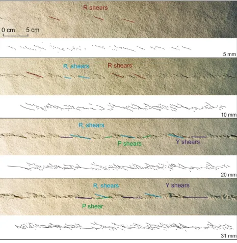
3.2.1.1 TALC and TALC_PIV

TALC and TALC_PIV are the simplest experiments in this study, and they are intended

as a baseline with which to compare the other, more complex models. They consist of a 2 cm

thick layer of talc sieved above the model’s “basement fault”, which was displaced at 1

mm/second for ~50 mm. The same experiment was performed twice, once recorded with

time-lapse photography (TALC) and once with the PIV system (TALC_PIV).

After 3-5 mm displacement, the first Riedel (R) shears initiate, which are oriented at

110-115° (measured clockwise from 0° as north, with the underlying fault striking 90°; see Figures

3.1, 3.2). At 10 mm displacement, lower angle Riedel shears (~105°, noted by Naylor et al., 1986, and identified here as RL shears following the terminology of Schreurs, 1994) start to

develop in limited areas, linking the initial fractures. By 20 mm, RL structures are widespread

throughout the fault zone, and P shears (85-95°) have begun to develop (Figure 3.1). Longer

fractures also develop, particularly in the 90-120° range (Figure 3.3). At this point, displacement

is partially occurring on Y shears, and by 30 mm displacement the fault is fully throughgoing,

though some inactive, more oblique structures are still visible (Figure 3.1). The longest fractures

(>2.5 cm) occur at these later strain intervals and all strike 90-100°, showing the progression

40

Figure 3.1. Images of TALC model at successive strain increments with corresponding fracture maps. Examples of R, RL, P, and Y shears are highlighted. Note progression from oblique structures to more