Cicada (Magicicada) Tree Damage Detection Based on UAV Spectral and 3D Data

http://www.scirp.org/journal/ns Natural Science, 2018, Vol. 10, (No. 1), pp: 31-44

https://doi.org/10.4236/ns.2018.101003 31 Natural Science

Cicada (

Magicicada

) Tree Damage Detection Based on

UAV Spectral and 3D Data

Ângela Maria Klein Hentz1,2, Michael P. Strager1

1_{Division of Resource Management, West Virginia University, Morgantown, WV, United States of}

America; 2_{Department of Forest Science, Federal University of Paraná, Curitiba, Brazil}

Correspondence to: Ângela Maria Klein Hentz,

Keywords: Photogrammetry, Insect Damage, 3D Dense Point Cloud

Received: December 28, 2017 Accepted: January 27, 2018 Published: January 30, 2018 Copyright © 2018 by authors and Scientific Research Publishing Inc.

This work is licensed under the Creative Commons Attribution International License (CC BY 4.0). http://creativecommons.org/licenses/by/4.0/

ABSTRACT

The periodical cicadas appear in regions of the United States in intervals of 13 or 17 years. During these intervals, deciduous trees are often impacted by the small cuts and eggs they lay in the outer branches which soon die off. Because this is such an infrequent occurrence and it is so difficult to assess the damage across large forested areas, there is little informa-tion about the extent of this impact. The use of remote sensing techniques has been proven to be useful in forest health management to monitor large areas. In addition, the use of Unmanned Aerial Vehicles (UAVs) has become a valuable tool for analysis. In this study, we evaluated the impact of the periodical cicada occurrence on a mixed hardwood forest using UAV imagery. The goal was to evaluate the potential of this technology as a tool for forest health monitoring. We classified the cicada impact using two Maximum Likelihood classi-fications, one using only the high resolution spectral derived from leaf-on imagery (MLC 1), and in the second we included the Canopy Height Model (CHM)—derived from leaf-on Digital Surface Model (DSM) and leaf-off Digital Terrain Model (DTM)—information in the classification process (MLC 2). We evaluated the damage percentage in relation to the total forest area in 15 circular plots and observed a range from 1.03% - 22.23% for MLC 1, and 0.02% - 10.99% for MLC 2. The accuracy of the classification was 0.35 and 0.86, for MLC 1 and MLC 2, based on the kappa index. The results allow us to highlight the importance of combining spectral and 3D information to evaluate forest health features. We believe this approach can be applied in many forest monitoring objectives in order to detect disease or pest impacts.

1. INTRODUCTION

The forest cover in the world was estimated at approximately 3999 million ha in 2015 of which only

https://doi.org/10.4236/ns.2018.101003 32 Natural Science

291 million ha were planted forests [1]. The forests provide many ecological, economic, social and cultural

benefits such as the regulation of hydrological cycles, wood production, soil protection, provision of food

and shelter for animals, recreation, carbon sequestration, and many others [2-4]. While forests suffer from

the pressure of population growth and deforestation [1, 5], they are also affected by insects, diseases,

ani-mals, weather events (as windstorm, ice, snow, and flooding) and others. The damage to the trees can

cause problems such as reduced growth, or even tree death [6], resulting in an impact to forest production

and ecological services.

Traditionally, the damage is evaluated by field inventories which are an expensive and

time-consuming activity, usually applied with subjective methods and have a limited extent [6, 7]. An

al-ternative option is to use remote sensing data to observe damages since spectral signatures can be observed

in vegetation under stress [8, 9]. There are at least three major strategies for using remote sensing to assess

forest damage: early damage detection, extent mapping, and damage quantification [6]. In forest health,

most studies have used remote sensing techniques to map forest conditions at a regional or stand level

[9-15]. Individual tree damage is often investigated for disturbance across stand level extents [16-18]. Few

studies have been able to examine individual branch scale disturbance because of the high spatial resolu-tion needed for detecresolu-tion.

The use of aerial imagery with unmanned aerial vehicles (UAVs) has greatly increased in the past five years across different fields of study because it has many advantages in comparison with other remote

sensing technologies. The main advantages of the UAV are the low cost of acquisition [19, 20], possibility

of frequent monitoring [21, 22], adaptability to carry various sensors, as thermal, infrared and

multispec-tral cameras or even Lidar scanners [19, 23-25], the high resolution obtained [19, 23, 26], and the devel-opment of processing software focused on the automatic reconstruction of surfaces using the UAV data

[27, 28]. An example of surface reconstruction has been in forest structure [29]. Studies have shown that

UAVs can help with species identification [30, 31], tree height [26, 32], crown delineation [26, 33, 34], and

forest health [35-37]. The use of UAVs has great potential for analyzing tree branch conditions as an early

detection of tree health [35]. Besides this potential, most of the studies applying UAV imagery to forest

health are based in multispectral bands, as near infrared and red edge, in addition to the traditional visible light bands [35-37] as presented in this paper.

This study examined forest health by analyzing the defoliation or blight caused by 17 years period

ci-cadas in a central Appalachian, USA forest plot. A preview of some results was presented in [38]. The

pe-riodical cicadas are from the genus Magicicada and are known as the species with the longest juvenile

de-velopment since they stay as nymphs on the underground being fed from root xylem fluids for 13 or 17

years [39], and emerge from the ground to become adults, reproduce, and die shortly after. They are

present in the eastern region of United States, and emerge each 13 years in the southern and midwestern

deciduous forest, and every 17 years in the northern and Great Plains states [40]. Along with the high

den-sity of cicadas presence, it is also been observed that the mortality of tree branches occurs due to cicada

oviposition in the trees [41]. The oviposition occurs primarily in young trees [41], and more in tree species

susceptible to oviposition, however, it does differ by year of the cicada brood [42].

The effect of the cicada’s oviposition in the trees is controversial [42], but it is generally considered

that they do not permanently damage the trees [41, 43, 44], even if some species result in a reduction in

growth after the oviposition [41, 43]. The dead branches can increase the susceptibility to diseases and

from other forest pests [42]. In this study, we wanted to investigate the utility of using UAV imagery to map

the extent of cicada damage in a mixed mesophytic hardwood stand in an Appalachian forest field plot.

2. MATERIALS AND METHODS

2.1. Study Area

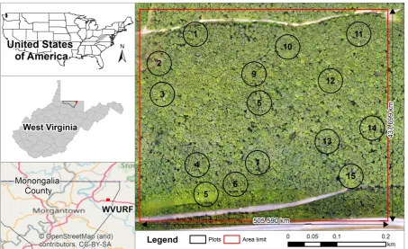
https://doi.org/10.4236/ns.2018.101003 33 Natural Science analyze the extent of the cicada damage, we selected one 21 ha site at the WVURF and collected aerial

im-agery by UAV (Figure 1).

In the 21 ha site we focused on 15 circular plots with a 25 m radius. In each of the plots we calculated the cicada damage as a percentage to the amount of forest. This site was selected because it has been mo-nitored for various forest management projects, and the collection of the imagery was coincident with the cicada occurrence. This site is representative of forest species in the region.

2.2. Data Collection

The imagery was collected over four seasons between 2016-2017, starting in Spring 2016. For this study we only utilized the images collected in the summer (July of 2016) and winter (March of 2017). The imagery collected in the summer was used to highlight the cicada occurrence, while the imagery from the winter was used to generate a digital terrain model.

The images were collected using a Phantom 3 professional UAV, equipped with a RGB (FC300X) camera. The FC300X camera sensor had dimensions of 6.317 mm × 4.738 mm and a focal length of 3.6 mm. The UAV the RGB camera was gimbal mounted in order to minimize vibrations in the camera.

Flight planning was done with the Maps Made Easy application, which allowed the selection of over-lap, height and direction of the flight. Images were captured using two flight directions (called double grid collection), which means that the area was flown two times (one north-south and another west-east). The double grid format is important in forests because the tree crown positions can obscure important fea-tures. We chose an overlap of 85% (lateral and forward) with an altitude of approximately 100 m.

Since the area had a large variation in elevation (mostly in the north-south direction), it was critical to integrate the mapped topography to assure the UAV followed the elevation contours. This option is avail-able in Maps Made Easy by the Terrain Awareness tool.

Figure 1. Study site location. Sources: top two left, vector files from the US Census Bureau website,

https://doi.org/10.4236/ns.2018.101003 34 Natural Science During the leaf-on phenology (summer), we obtained 1673 images as compared to the winter leaf-off collection of 971. The smaller number of images during the leaf-off collection was due to a single grid ac-quisition of the imagery processed. For the leaf-off data collection, the illumination conditions were highly variable and therefore we only processed one dataset.

In addition to the imagery collection, we also placed targets and collected control and check points during the image processing. We placed 12 targets in the area and we used 3 as check points, while the

other 9 were used as control points. The targets were made using 0.38 m2 _{plywood panels painted in black}

and white. These targets were placed in the roads at north and south of the site, as well inside the forest. The placement of targets inside the forest was a challenge since it required locating canopy gaps to allow their viewing during the leaf-on imagery. The coordinates of the targets were obtained using an iGage X900S-OPUS GNSS static receiver, mounted in a tripod at a standard height of 2 m above the ground. For each point the receiver recorded at least 15 minutes of data positions, and in some cases, we collected 2 hours (when the 15 min did not provide a solution). The recorded data was sent to the Online Positioning User Service (OPUS), which returned the real point position calculated using GPS and corrections calcu-lated by available CORS (Continuously Operating Reference Station) stations.

2.3. Image Processing

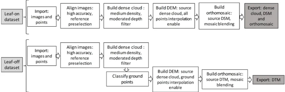
After data collection, the images were processed using Agisoft Photoscan Professional Version 1.2.6. Each dataset (leaf-on and leaf-off seasons) was processed separately. The processing was similar for both datasets, but the leaf-off dataset required extra steps. The images were aligned using the ground control point and the coordinates from the pictures (from the UAV onboard GPS). The alignment step was done using the high accuracy setting on Agisoft. The dense cloud was created using the Medium density and Moderate depth filtering.

We generated a digital surface model (DSM) from the dense point cloud. For the leaf-on dataset, the DSM was built using all the points, while for the leaf-off this process was done using only the points classi-fied as ground. The leaf-off point cloud classification was accomplished using a tool available on Agisoft, which considered the parameters maximum angle, maximum distance and cell size. The classification was improved by manually selecting groups of points and placing them in the correct class. This way instead of a DSM we obtained a digital terrain model (DTM) of the area.

Lastly, we generated an orthomosaic using the DSM as a surface for the leaf-on dataset, and DTM for leaf-off dataset. After the orthomosaic generation, all the products (dense clouds, DSM and DTM, and the orthomosaics) were exported. During the steps of DMS/DTM and orthomosaic generation we selected the

best possible resolution which was 3 cm for all data. The processing is summarized in Figure 2.

Figure 2. UAV processing steps applied on the leaf-on and leaf-off UAV imagery datasets to obtain

https://doi.org/10.4236/ns.2018.101003 35 Natural Science

2.4. Cicada Damage Detection

The cicada damage was determined using the Maximum Likelihood Classification (MLC) method in two different configurations. In the first classification (MLC 1), we used only the orthomosaic to classify the damage, which meant a spectral response of the image. In a second attempt (MLC 2), we included the altitude of the area within the orthomosaic. Therefore, in this second situation the classification was made using spectral and elevation values. We hypothesized that the high resolution orthomosaic generated from the UAV imagery and the 3D information obtained from these vehicles could be very useful to many re-mote sensing classification applications.

For the first classification (MLC 1), we clipped the orthomosaic to the study area, selected samples for all the classes of interest, and generated a signature file to execute the MLC. For the second classification (MLC 2), we first created a Canopy Height Model (CHM), by subtracting the DTM values from the DSM. In some locations, we observed negative values as a result of small variations in the area. These anomalies were converted to zero by a search and replace. The CHM was added to the orthomosaic and then we ap-plied the same classification method to the MLC 1. In both cases we used the same samples, we only gen-erated a different signature file.

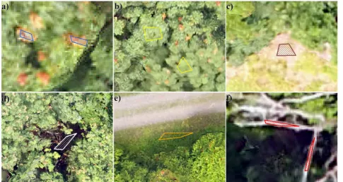
To classify healthy and damaged forest extents, we created six classes: Damage, the leaves that are dead because of the cicada oviposition; Healthy forest, all the forest that does not present signals of dam-age; Ground, the roads and large open spaces in the canopy that penetrate to the ground; Shadows, all dark regions created by the shadows of the trees in the images; Small vegetation, the scrubs and bushes mostly founded in the edge between the forest and the roads, as well portions of grass; and Wood, representing the dead trees where only the trunks are visible. Examples of the classes and selected samples are presented

in Figure 3.

Figure 3. Training samples collected and utilized in Maximum Likelihood Classification. In (a) the

https://doi.org/10.4236/ns.2018.101003 36 Natural Science We used 50 random points to calculate the accuracy of the classification. These points were randomly distributed throughout the area. We derived features from the two classifications (MLC 1 and MLC 2) and the real feature (classified by visual interpretation) in each point position. With these values, we built a confusion matrix and calculated the Kappa index.

To better evaluate the severity of the cicada damage in the forest, we calculated the percentage to the total of forest in the 15 plots.

3. RESULTS

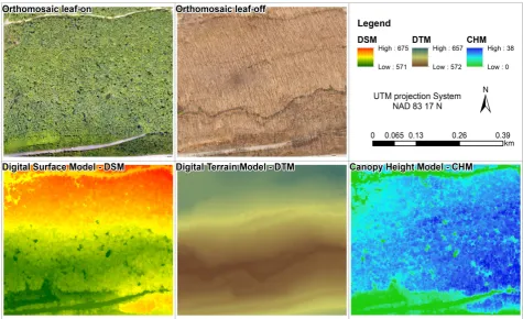
The leaf-on and leaf-off imagery produced a complete dataset for the study area. The leaf-on imagery provided a high resolution orthomosaic where we could observe the cicada damage, a 3D point cloud and a DSM. The ground resolution obtained from the leaf-on imagery was 3.03 cm/pix, and the DSM

pre-sented a resolution of 12.1 cm/pix with 68.2 points/m2_.

The leaf-off imagery was used to create a DTM for the MLC 2, yet this dataset also created an ortho-mosaic and a 3D point cloud. The leaf-off imagery presented a ground resolution of 4.85 cm/pix, the DTM

presented a resolution of 19.4 cm/pix, and a dense point density of 26.5 points/m2_{. The accuracy of the}

processing by the control and check points is shown in Table 1.

In Figure 4, the results are presented from the image processing of both datasets, leaf-on

(orthomo-saic and DSM) and leaf-off (orthomo(orthomo-saic and DTM), as well the CHM from the DSM-DTM operation. Based on this data, we performed the two classifications and found the values for each category by

plot. This information is presented in Table 2 and Table 3, respectively for MLC 1 and MLC 2, as well in

Figure 5.

The classification accuracy based on the Kappa index was calculated as 0.35 for MLC 1, while it was

0.86 for MLC 2. The confusion matrix is presented in Table 4.

Figure 4. Orthomosaics, DSM, DTM and CHM obtained from the UAV imagery leaf-on and leaf-off

https://doi.org/10.4236/ns.2018.101003 37 Natural Science

Table 1. Processing accuracy.

Dataset Point type X error (m) Y error (m) Z error (m) Total (m) Total (pixel)

Leaf-on Control 2.32 1.48 5.25 5.93 3.70

Leaf-on Check 1.03 0.85 7.07 7.20 7.08

Leaf-off Control 2.03 1.33 4.55 5.15 0.87

Leaf-off Check 1.29 1.54 6.85 7.13 1.05

Table 2. Classification results for MLC 1, using only orthomosaic.

Plot Forest Small Veg. Shadows Ground Wood

Damage Healthy % Damage

1 113.74 1007.55 10.14 604.15 150.00 8.60 69.38

2 240.53 841.68 22.23 630.06 111.52 8.63 120.98

3 75.70 1039.57 6.79 709.21 87.21 0.37 41.33

4 35.07 1477.47 2.32 292.84 130.67 0.68 16.80

5 8.60 335.70 2.50 1564.60 24.10 15.26 5.19

6 10.95 1053.61 1.03 728.70 153.12 0.01 7.04

7 48.26 1496.86 3.12 224.85 161.87 2.09 19.49

8 36.11 1303.52 2.70 434.77 155.30 0.01 23.68

9 95.40 834.63 10.26 831.86 155.53 0.19 35.78

10 42.60 1304.00 3.16 467.41 109.30 0.89 29.22

11 48.69 1370.99 3.43 367.06 133.43 0.52 32.81

12 32.63 1076.15 2.94 732.22 95.20 0.01 17.29

13 27.68 1431.76 1.90 318.00 155.11 0.03 20.93

14 39.30 1199.05 3.17 569.78 122.92 0.45 21.92

15 34.69 1281.73 2.63 453.67 124.47 10.77 48.08

Total 889.96 17,054.26 4.96 8929.20 1869.75 48.50 509.91

Total areaa _{0.93 12.51 6.90 (5.29) 6.04 1.47 0.42 0.53}

a_{Results for plots and total are in m}2_{, while the result for the total area is in ha. Value in brackets is the}

standard deviation.

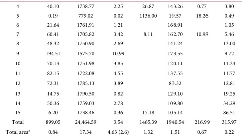
Table 3. Classification results for MLC 2, using orthomosaic and CHM.

Plot Forest Small Veg. Shadows Ground Wood

Damage Healthy % Damage

1 71.52 1488.96 4.58 128.32 185.80 51.56 27.31

2 62.44 1404.24 4.26 148.92 145.36 135.42 57.05

https://doi.org/10.4236/ns.2018.101003 38 Natural Science Continued

4 40.10 1738.77 2.25 26.87 143.26 0.77 3.80

5 0.19 779.02 0.02 1136.00 19.57 18.26 0.49

6 21.64 1761.91 1.21 168.91 1.05

7 60.41 1705.82 3.42 8.11 162.70 10.98 5.46

8 48.32 1750.90 2.69 141.24 13.00

9 194.51 1575.70 10.99 173.55 9.72

10 70.13 1751.98 3.85 120.11 11.24

11 82.15 1722.08 4.55 137.55 11.77

12 72.31 1785.13 3.89 83.32 12.81

13 14.75 1790.50 0.82 129.10 19.25

14 50.36 1759.03 2.78 109.80 34.29

15 6.20 1738.46 0.36 17.18 105.14 86.51

Total 899.05 24,464.59 3.54 1465.39 1940.54 216.99 315.97

Total areaa _{0.84 17.34 4.63 (2.6) 1.32 1.51 0.67 0.22}

a_{Results for plots and total are in m}2_{, while the result for the total area is in ha. Value in bracket is the}

standard deviation.

Table 4. Confusion matrix from the classifications MLC 1 and MLC 2.

Class Real class Class Real class

D HF SV S G W ∑ D HF SV S G W ∑

M LC 1 Cl as sif ic at io n

D 2 2 4

M LC 2 Cl as sif ic at io n

D 2 2

HF 26 1 2 29 HF _{1 36 1 38}

SM 1 9 1 11 SM 3 1 4

S 1 1 2 S 2 2

G 1 1 G 3 3

W 1 1 1 3 W 1 1

∑ 3 36 3 3 4 1 50 ∑ 3 36 3 3 4 1 50

Where: D = Damage; HF = Healthy forest; SM = Small vegetation; S = Shadows; G = Ground; W = Wood.

Based on the results presented in the Table 4, as well in the Figure 5, we can conclude that some

https://doi.org/10.4236/ns.2018.101003 39 Natural Science

Figure 5. Maximum likelihood classification results on the cicada damage detection using only

spectral information (MCL 1), and using spectral and height information (MCL 2).

4. DISCUSSION

This study highlighted the importance of additionally produced UAV outputs for classifying a unique forest disturbance. Specifically, the inclusion of DTM and DSM to create a CHM proved to be critical for the classification of the cicada damage. A similar approach was earlier applied using combinations of

high-resolution imagery and Lidar and was found to be successful in many applications [15, 45-47]. We

believe that the UAV data can be used in many of these situations, being a source of 3D and spectral in-formation from the same source, reducing costs and time of acquisition.

Our result helps to bring attention to the use of UAV imagery for many landscape classification stu-dies in which a unique feature at a high resolution is required for mapping. This may include not only ve-getated features but any structure in which the goal is to better classify its extent or compare a location to its neighbors such as in stream riparian corridor analysis for the purpose of additional derivatives such as flow direction, accumulation, heat load index, topographic moisture index, and other geomorphic

attributes [22, 48-50]. Compared to earlier remote sensing platforms in which only satellite or fixed wing

aircraft provide spectral information, the inclusion of the structure from motion output from UAVs makes it a unique and very promising alternative to the traditional aerial imagery sources. This is especially rele-vant as more and more UAV platforms, camera components, and flight times improve.

While structure from motion was shown to be important for detecting the cicada impact in this study, it should be noted that the approach does have its limitations. The calculation of the point cloud can result

in elevation values with accuracies dependent on ground cover and topographic structure [28, 48, 50-52].

Depending on the study, it is critical to acknowledge this limitation. Better positional control and

https://doi.org/10.4236/ns.2018.101003 40 Natural Science combined with Lidar data to better capture the range of elevation values. This is primarily due to the laser pulses ability to penetrate canopy or understory features [26, 28, 54].

However, with Lidar there is a significant time and money investment required to acquire the

tech-nology especially when the structure from motion may suffice [52, 55]. The value of the information must

be considered in future flight and project planning. This study suggests that future research look at the contributions that structure from motion compared to Lidar data provides to make the most cost-effective decisions regarding their use. We believe that one answer or threshold will not always suffice due to the different variable inputs that make up that decision making process. Fortunately, as technology improves, this decision may become easier and the resource management questions that this technology helps to answer will become more widespread across applications.

5. CONCLUSION

In this study, we highlight the benefits of using UAV data as a tool to monitor forest health. The po-tential of this technology does not only exist in the low-cost acquisition of high-resolution imagery, but also in the integration of this data with advances in processing techniques that allow the extraction of 3D information.

This technology is capable to obtain both structural and visual information and to characterize the physiologic status of the forest. The information can be applied in future studies to detect early occurrence of diseases and pests. Since early detection is critical, the approach can be irreplaceable tool for forest management.

ACKNOWLEDGEMENTS

This paper is based upon work supported by the National Science Foundation under Cooperative Agreement Number OIA-1458952. Any opinions, findings, and conclusions or recommendations ex-pressed in this material are those of the author(s) and do not necessarily reflect the views of the National Science Foundation. The work was also supported by the USDA National Institute of Food and Agricul-ture, Hatch project, and the West Virginia Agricultural and Forestry Experiment Station.

REFERENCES

1. FAO (2015) Global Forest Resources Assessment. Food and Agriculture Organization of the United Nations,

Rome.

2. Krieger, D. (2001) Economic Value of Forest Ecosystem Services: A Review. The Wilderness Society,

Washing-ton DC.

3. Wunder, S. and Thorsen, B.J. (2014) Ecosystem Services and Their Quantificatio. In: Thorsen, B.J., Mavsar, R.,

Tyrväinen, L., Prokofieva, I. and Stenger, A., Ed., The Provision of Forest Ecosystem Services. Volume I:

Quan-tifying and Valuing Non-Marketed Ecosystem Services, European Forest Institute, Finland.

4. Binder, S., Haight, R.G., Polasky, S., Warziniack, T., Mockrin, M.H., Deal, R.L. and Arthaud, G. (2017)

Assess-ment and Valuation of Forest Ecosystem Services: State of the Science Review. Forest Service, Northern Re-search Station, General Technical Report NRS-170.

5. Defries, R.S., Rudel, T., Uriarte, M. and Hansen, M. (2010) Deforestation Driven by Urban Population Growth

and Agricultural Trade in the Twenty-First Century. Nature Geoscience, 3, 178-181. https://doi.org/10.1038/ngeo756

6. Franklin, S.E. (2001) Remote Sensing for Sustainable Forest Management. Lewis Publishers, New York.

https://doi.org/10.1201/9781420032857

7. Ferretti, M. (1997) Forest Health Assessment and Monitoring—Issues for Consideration. Environmental

https://doi.org/10.4236/ns.2018.101003 41 Natural Science

8. Rock, B.N., Vogelmann, J.E., Williams, D.L., Vogelmann, A.F. and Hoshizaki, T. (1986) Remote Detection of

Forest Damage. Bioscience, 36, 439-445. https://doi.org/10.2307/1310339

9. Cielsa, W.M. (2000) Remote Sensing in Forest Health Protection. USDA Forest Service, Remote Sensing

Appli-cations Center and Forest Health Technology Enterprise Team. FHTET Report No. 00-03.

10. Hatala, J.A., Crabtree, R.L., Halligan, K.Q. and Moorcroft, P.R. (2010) Landscape-Scale Patterns of Forest Pest

and Pathogen Damage in the Greater Yellowstone Ecosystem. Remote Sensing of Environment, 114, 375-384.

https://doi.org/10.1016/j.rse.2009.09.008

11. Meng, J., Li, S., Wang, W., Liu, Q., Xie, S. and Ma, W. (2016) Mapping Forest Health Using Spectral and

Tex-tural Information Extracted from SPOT-5 Satellite Images. Remote Sensing, 8, 719-739. https://doi.org/10.3390/rs8090719

12. Olsson, P.O., Jönsson, A.M. and Eklundh, L. (2012) A New Invasive Insect in Sweden—Physokermesinopinatus:

Tracing Forest Damage with Satellite Based Remote Sensing. Forest Ecology and Management,285, 29-37.

https://doi.org/10.1016/j.foreco.2012.08.003

13. Wulder, M.A., Dymond, C.C., White, J.C., Leckie, D.G. and Carroll, A.L. (2006) Surveying Mountain Pine

Beetle Damage of Forests: A Review of Remote Sensing Opportunities. Forest Ecology and Management, 221,

27-41. https://doi.org/10.1016/j.foreco.2005.09.021

14. King, D.J., Olthof, I., Pellikka, P.K.E., Seed, E.D. and Butson, C. (2005) Modelling and Mapping Damage to

Fo-rests from an Ice Storm Using Remote Sensing and Environmental Data. Natural Hazards, 35, 321-342.

https://doi.org/10.1007/s11069-004-1795-4

15. Honkavaara, E., Litkey, P. and Nurminen, K. (2013) Automatic Storm Damage Detection in Forests Using

High-Altitude Photogrammetric Imagery. Remote Sensing, 5, 1405-1424. https://doi.org/10.3390/rs5031405

16. White, J.C., Wulder, M.A., Brooks, D., Reich, R. and Wheate, R.D. (2005) Detection of Red Attack Stage

Moun-tain Pine Beetle Infestation with High Spatial Resolution Satellite Imagery. Remote Sensing of Environment, 96, 340-351. https://doi.org/10.1016/j.rse.2005.03.007

17. Wulder, M.A., White, J.C., Coggins, S., Ortlepp, S.M., Coops, N.C., Heath, J. and Mora, B. (2012) Digital High

Spatial Resolution Aerial Imagery to Support Forest Health Monitoring: The Mountain Pine Beetle Context.

Journal of Applied Remote Sensing,6, 62510-62527.

18. Wulder, M.A., Ortlepp, S.M., White, J.C., Coops, N.C. and Coggins, S.B. (2009) Monitoring the Impacts of

Mountain Pine Beetle Mitigation. Forest Ecology and Management,258, 1181-1187.

https://doi.org/10.1016/j.foreco.2009.06.008

19. Wallace, L., Lucieer, A., Watson, C. and Turner, D. (2012) Development of a UAV-LiDAR System with

Appli-cation to Forest Inventory. Remote Sensing,4, 1519-1543.https://doi.org/10.3390/rs4061519

20. Nex, F. and Remondino, F. (2014) UAV for 3D Mapping Applications: A Review. Applied Geomatics, 6, 1-15.

https://doi.org/10.3390/rs4061519

21. Salamí, E., Barrado, C. and Pastor, E. (2014) UAV Flight Experiments Applied to the Remote Sensing of

Vege-tated Areas. Remote Sensing,6, 11051-11081. https://doi.org/10.3390/rs61111051

22. Murfitt, S.L., Allan, B.M., Bellgrove, A., Rattray, A., Young, M.A. and Ierodiaconou, D. (2017) Applications of

Unmanned Aerial Vehicles in Intertidal Reef Monitoring. Scientific Reports,7, Article No. 10259. https://doi.org/10.1038/s41598-017-10818-9

23. Zarco-Tejada, P.J., Diaz-Varela, R., Angileri, V. and Loudjani, P. (2014) Tree Height Quantification using Very

High Resolution Imagery Acquired from an Unmanned Aerial Vehicle (UAV) and Automatic 3D

Pho-to-Reconstruction Methods. European Journal of Agronomy,55, 89-99.

https://doi.org/10.4236/ns.2018.101003 42 Natural Science

24. Tang, L. and Shao, G. (2015) Drone Remote Sensing for Forestry Research and Practices. Journal of Forestry

Research,26, 791-797. https://doi.org/10.1007/s11676-015-0088-y

25. Colomina, I. and Molina, P. (2014) Unmanned Aerial Systems for Photogrammetry and Remote Sensing: A

Re-view. ISPRS Journal of Photogrammetry and Remote Sensing,92, 79-97.

https://doi.org/10.1016/j.isprsjprs.2014.02.013

26. Wallace, L., Lucieer, A., Malenovsky, Z., Turner, D. and Vopenka, P. (2016) Assessment of Forest Structure

us-ing Two UAV Techniques: A Comparison of Airborne Laser Scannus-ing and Structure from Motion (SfM) Point Clouds. Forests,7, 1-16. https://doi.org/10.3390/f7030062

27. Verhoeven, G. (2011) Taking Computer Vision Aloft-Archaeological Three-Dimensional Reconstructions from

Aerial Photographs with Photoscan. Archaeological Prospection,62, 61-62. https://doi.org/10.1002/arp.399

28. Dandois, J.P. and Ellis, E.C. (2010) Remote Sensing of Vegetation Structure using Computer Vision. Remote

Sensing,2, 1157-1176. https://doi.org/10.3390/rs2041157

29. Chisholm, R.A., Cui, J., Lum, S.K.Y. and Chen, B.M. (2013) UAV LiDAR for Below-Canopy Forest Surveys.

Journal of Unmanned Vehicle Systems, 1, 61-68.https://doi.org/10.1139/juvs-2013-0017

30. Puttonen, E., Litkey, P. and Hyyppä, J. (2010) Individual Tree Species Classification by Illuminated-Shaded Area

Separation. Remote Sensing,2, 19-35. https://doi.org/10.3390/rs2010019

31. Lisein, J., Michez, A., Claessens, H. and Lejeune, P. (2015) Discrimination of Deciduous Tree Species from Time

Series of Unmanned Aerial System Imagery. PLoS ONE, 10, e0141006.

https://doi.org/10.1371/journal.pone.0141006

32. Hung, C., Bryson, M. and Sukkarieh, S. (2012) Multi-Class Predictive Template for Tree Crown Detection.

ISPRS Journal of Photogrammetry and Remote Sensing,68, 170-183.

https://doi.org/10.1016/j.isprsjprs.2012.01.009

33. Díaz-Varela, R., de la Rosa, R., León, L. and Zarco-Tejada, P. (2015) High-Resolution Airborne UAV Imagery to

Assess Olive Tree Crown Parameters using 3D Photo Reconstruction: Application in Breeding Trials. Remote

Sensing,7, 4213-4232. https://doi.org/10.3390/rs70404213

34. Panagiotidis, D., Abdollahnejad, A., Surový, P. and Chiteculo, V. (2016) Determining Tree Height and Crown

Diameter from High-Resolution UAV Imagery. International Journal of Remote Sensing,38, 2392-2410.

https://doi.org/10.1080/01431161.2016.1264028

35. Dash, J.P., Watt, M.S., Pearse, G.D., Heaphy, M. and Dungey, H.S. (2017) Assessing Very High Resolution UAV

Imagery for Monitoring Forest Health during a Simulated Disease Outbreak. ISPRS Journal of Photogrammetry

and Remote Sensing,131, 1-14. https://doi.org/10.1016/j.isprsjprs.2017.07.007

36. Näsi, R., Honkavaara, E., Lyytikäinen-Saarenmaa, P., Blomqvist, M., Litkey, P., Hakala, T., Viljanen, N.,

Kanto-la, T., Tanhuanpää, T. and Holopainen, M. (2015) Using UAV-Based Photogrammetry and Hyperspectral

Im-aging for Mapping Bark Beetle Damage at Tree-Level. Remote Sensing,7, 15467-15493.

https://doi.org/10.3390/rs71115467

37. Lehmann, J.R.K., Nieberding, F., Prinz, T. and Knoth, C. (2015) Analysis of Unmanned Aerial System-Based

CIR Images in Forestry—A New Perspective to Monitor Pest Infestation Levels. Forests,6, 594-612. https://doi.org/10.3390/f6030594

38. Hentz, A.M.K. and Strager, M.P. (2017) Cicada Damage Detection Based on UAV Spectral and 3D Data.

Pro-ceeding of Silvilaser, Blacksburg, 10-12 October 2017, 95-96.

39. Williams, K.S. and Simon, C. (1995) The Ecology, Behavior, and Evolution of Periodical Cicadas. Annual

Re-view of Entomology,40, 269-295. https://doi.org/10.1146/annurev.en.40.010195.001413

https://doi.org/10.4236/ns.2018.101003 43 Natural Science J.E. and Simon, C. (2017) A GIS-Based Map of Periodical Cicada Brood XIII in 2007, with Notes on Adjacent Populations of Broods III and X (Hemiptera: Magicicada spp.). American Entomologist,62, 241-246.

https://doi.org/10.1093/ae/tmw077

41. Clay, K., Shelton, A.L. and Winkle, C. (2009) Effects of Oviposition by Periodical Cicadas on Tree Growth.

Ca-nadian Journal of Forest Research,39, 1688-1697. https://doi.org/10.1139/X09-090

42. Clay, K., Shelton, A.L. and Winkle, C. (2009) Differential Susceptibility of Tree Species to Oviposition by

Pe-riodical Cicadas. Ecological Entomology,34, 277-286. https://doi.org/10.1111/j.1365-2311.2008.01071.x

43. Speer, J.H., Clay, K., Bishop, G. and Creech, M. (2010) The Effect of Periodical Cicadas on Growth of Five Tree

Species in Midwestern Deciduous Forests. The American Midland Naturalist, 164, 173-186. https://doi.org/10.1674/0003-0031-164.2.173

44. Flory, S.L. and Mattingly, W.B. (2008) Response of Host Plants to Periodical Cicada Oviposition Damage.

Oe-cologia, 156, 649-656. https://doi.org/10.1007/s00442-008-1016-z

45. Chen, Y., Su, W., Li, J. and Sun, Z. (2009) Hierarchical Object Oriented Classification using Very High

Resolu-tion Imagery and LIDAR Data over Urban Areas. Advances in Space Research,43, 1101-1110.

https://doi.org/10.1016/j.asr.2008.11.008

46. Ke, Y., Quackenbush, L.J. and Im, J. (2010) Synergistic Use of QuickBird Multispectral Imagery and LIDAR

Data for Object-Based Forest Species Classification. Remote Sensing of Environment,114, 1141-1154. https://doi.org/10.1016/j.rse.2010.01.002

47. Dalponte, M., Bruzzone, L. and Gianelle, D. (2012) Tree Species Classification in the Southern Alps Based on

the Fusion of Very High Geometrical Resolution Multispectral/Hyperspectral Images and LiDAR Data. Remote

Sensing of Environment,123, 258-270. https://doi.org/10.1016/j.rse.2012.03.013

48. Tamminga, A., Hugenholtz, C., Eaton, B. and Lapointe, M. (2015) Hyperspatial Remote Sensing of Channel

Reach Morphology and Hydraulic Fish Habitat using an Unmanned Aerial Vehicle (UAV): A First Assessment in the Context of River Research and Management. River Research and Applications,31, 379-391.

https://doi.org/10.1002/rra.2743

49. Lucieer, A., Turner, D., King, D.H. and Robinson, S.A. (2014) Using an Unmanned Aerial Vehicle (UAV) to

Capture Micro-Topography of Antarctic Moss Beds. International Journal of Applied Earth Observation and

Geoinformation,27, 53-62. https://doi.org/10.1016/j.jag.2013.05.011

50. Smith, M.W. and Vericat, D. (2015) From Experimental Plots to Experimental Landscapes: Topography,

Ero-sion and Deposition in Sub-Humid Badlands from Structure-from-Motion Photogrammetry. Earth Surface

Processes and Landforms,40, 1656-1671. https://doi.org/10.1002/esp.3747

51. Mancini, F., Dubbini, M., Gattelli, M., Stecchi, F., Fabbri, S. and Gabbianelli, G. (2013) Using Unmanned Aerial

Vehicles (UAV) for High-Resolution Reconstruction of Topography: The Structure from Motion Approach on

Coastal Environments. Remote Sensing,5, 6880-6898.https://doi.org/10.3390/rs5126880

52. Hugenholtz, C.H., Whitehead, K., Brown, O.W., Barchyn, T.E., Moorman, B.J., Leclair, A., Riddell, K. and

Hamilton, T. (2013) Geomorphological Mapping with a Small Unmanned Aircraft System (sUAS): Feature

De-tection and Accuracy Assessment of a Photogrammetrically-Derived Digital Terrain Model. Geomorphology,

194, 16-24. https://doi.org/10.1016/j.geomorph.2013.03.023

53. Harwin, S. and Lucieer, A. (2012) Assessing the Accuracy of Georeferenced Point Clouds Produced via

Mul-ti-View Stereopsis from Unmanned Aerial Vehicle (UAV) Imagery. Remote Sensing,4, 1573-1599.

https://doi.org/10.3390/rs4061573

54. Mathews, A.J. and Jensen, J.L.R. (2013) Visualizing and Quantifying Vineyard Canopy LAI using an Unmanned

https://doi.org/10.4236/ns.2018.101003 44 Natural Science

2164-2183. https://doi.org/10.3390/rs5052164

55. Dandois, J.P. and Ellis, E.C. (2013) High Spatial Resolution Three-Dimensional Mapping of Vegetation Spectral

Dynamics using Computer Vision. Remote Sensing of Environment,136, 259-276.