System identification and its applications, with emphasis on direction dependent processes

(1)

University of Warwick institutional repository: http://go.warwick.ac.uk/wrap

A Thesis Submitted for the Degree of PhD at the University of Warwick

http://go.warwick.ac.uk/wrap/66737

This thesis is made available online and is protected by original copyright. Please scroll down to view the document itself.

(2)

•

o

WA~)CK

System Identification and its

Applications, with Emphasis on

Direction-dependent Processes

AiHui Tan

A thesis submitted in partial fulfilment of the requirements

for the degree of Doctor of Philosophy

University

of Warwick

School of Engineering

(3)

(4)

Table o/Contents

.

Acknowledgements ... Vl Declaration ... VII

...

Summary of the Thesis ... VIII Glossary of Abbreviations Used ... ix

CHAPTER 1 - Introduction ... 1

CHAPTER 2 - Design of Pseudo-random Perturbation Signals for System Identification ... 1 0 2.1 Abstract ... 11

2.2 Introduction ... 11

2.3 Design ofa New MATLAB Routine ... 13

2.3.1 Generation of Maximum Length Binary Signals and the Design of Related Functions ... 13

2.3.1.1 Generation of Maximum Length Binary Signals ... 13

2.3.1.2 Calculation of Resulting Shift due to Shift-and-add Property ... 14

2.3.1.3 Measures of Rejection of Unsystematic Errors ... 15

2.3.2 Other Classes of Signal Available ... 16

2.3.3 Other Functions Available ... 18

2.3.4 List of Functions ... 24

2.4 Extension to Multi-level Pseudo-random Signals ... 27

2.4.1 Introduction to Nonlinear System Identification ... 27

2.4.2 Properties of Multi-level Signals ... 28

2.4.2.1 Three-level Signals ... 28

2.4.2.2 Four-level Signals ... 29

2.4.2.3 Five-level Signals ... 31

2.4.3 Design of Multi-level Signals for the Identification of Hammer stein Models ... 32

2.5 Conclusions ... 38

CHAPTER 3 - Detection of Departure from Linearity for Processes with Direction-dependent Dynamics ... 41

3.1 Abstract ... 42

3.3 Process Simulation using MATLAB ... 43

3.4 Detection of Direction-dependent Dynamics ... 45

3.4.1 Process with First Order Dynamics ... .45

(5)

Table o/Contents 11

3.4.1.2 Detection using Multi-level Maximum Length Signals ... 50

3.4.1.3 Detection using Multisines ... 55

3.4.2 Process with Second Order Dynamics ... 59

3.4.2.1 Detection using Pseudo-random Binary Signals ... 59

3.4.2.2 Detection using Multi-level Maximum Length Signals ... 63

3.4.2.3 Detection using Multisines ... 65

CHAPTER 4 - Estimation of Linear Dynamics for Processes with Direction-dependent Dynamics ... 67

4.2 Parameter Estimation Methods ... 68

4.2.1 Estimation using System Identification Toolbox ... 68

4.2.2 Estimation using Frequency Domain System Identification Toolbox ... 70

4.2.3 Estimation using Correlation Analysis ... 71

4.3 Estimation of Linear Dynamics ... 72

4.3.1 Process with First Order Dynamics ... 72

4.3.2 Process with Second Order Dynamics ... 78

4.4 Estimation of Overall Gain for Processes with Direction-dependent Gains ... 85

4.4.1 Introduction ... 85

4.4.2 First Order Process ... 85

4.4.3 Second Order Process ... 88

CHAPTER 5 - The Use of Wiener Models to Describe Systems with Direction-dependent Dynamics ... 94

5.1 Abstract ... 95

5.3 First Order Direction-dependent Process ... 96

5.3.1 Derivation of Process Output ... 96

5.3.2 Derivation of Cross correlation Function using Maximum Length Binary Signals ... 99

5.3.3 Derivation of Cross correlation Function using Inverse-repeat Maximum Length Binary Signals ... 101

5.4 Wiener Process with First Order Dynamics ... 104

5.4.1 Derivation of Crosscorrelation Function using Maximum Length Binary Signals ... 104

5.4.2 Derivation of Crosscorrelation Function using Inverse-repeat Maximum Length Binary Signals ... 108

5.5 Comparison between First Order Direction-dependent and Wiener Processes ... 109

(6)

Table of Contents iii

5.6 Extension to Second Order Processes ... 118

CHAPTER 6 - Modelling of Direction-dependent Dynamic Processes : A Comparison of Wiener Models and Neural Networks ... 128

6.1 Abstract ... 129

6.2 Neural Network Architecture ... 12 9 6.3 Modelling First Order Direction-dependent Process ... 130

6.4 Modelling Second Order Direction-dependent Process ... 139

6.5 Practical Application using Electronic Nose ... 145

6.5.1 Model of the Gas Sensor ... 145

6.5.2 Experimental Setup ... 146

6.S.3 Detection and Estimation of Direction-dependent Dynamics ... 146

6.S.4 Modelling of Direction-dependent Dynamics ... ISO 6.6 Conclusions ... IS4 CHAPTER 7 - Control of Processes with Direction-dependent Dynamics ... 156

7.1 Introduction ... IS7 7.2 Control of Processes with the Same Gain in Both Directions ... 158

7.2.1 Control of First Order Process ... 1S8 7.2.1.1 Control Using PID ... 158

7.2.1.2 Alternative Implementations of the Derivative Term ... 161

7.2.1.3 Effects of Varying Controller Gain ... 165

7.2.1.4 Effects of Varying Controller Period ... 167

7.2.2 Control of Second Order Process ... 169

7.2.2.1 Comparison of Performance of Three Different Controllers ... 169

7.2.2.2 Effects of Varying Controller Gain ... 172

7.2.2.3 Effects of Varying Controller Period ... 173

7.3 Control of Processes with Direction-dependent Gains ... 175

7.3.1 Control of First Order Process ... 175

7.3.1.1 Control Using PID ... 175

7.3.1.2 Control Using PID with Moving A verager ... 179

7.3.2 Control of Second Order Process ... 182

7.3.2.1 Control Using PID ... 182

7.3.2.2 Control Using PID with Moving Averager ... 182

CHAPTER 8 - Autotune Control of Processes with Significant Dead Time ... 188

8.3 Signal Design ... 191

8.4 Smith Predictor ... 192

(7)

Table oJContents IV

8.5.1 PI Control ... 193

8.5.2 The Dahlin Controller ... 194

8.5.3 Simulation Results ... 195

8.5.3.1 Parameter Estimation ... 195

8.5.3.2 Controller Responses ... 1 97 8.6. Controller Robustness ... 202

8.7 Control ofa Second Order Process ... 204

8.7.1 PI Control ... 204

8.7.2 Simulation Results ... 205

8.7.2.1 Parameter Estimation ... 205

8.7.2.2 Controller Responses ... 207

8.7.3 Controller Robustness ... 211

8.7.4 Identification and Control of Second Order Underdamped Processes ... 211

8.8 Reduced Order Modelling ... 212

8.8.1 High Order Process ... 213

8.8.2 Non-minimum Phase Process ... 216

8.9 Application Example ... 219

CHAPTER 9 - Identification of Wiener-Hammerstein Models using Linear Interpolation in the Frequency Domain (LIFRED) ..•...••.•.•....•....•.•.•...•...•. 223

9.3 Volterra Kernels ... 226

9.4 Identification of Linear Subsystems using Linear Interpolation in the Frequency Domain (LIFRED) ... 227

9.4.1 Signal Design ... 227

9.4.2 Calculation of the Frequency Response Gain of the Second Linear Subsystem ... 230

9.4.3 Calculation of the Frequency Response Gain of the First Linear Subsystem ... 232

9.4.4 Simultaneous Calculation of the Frequency Response Phases of the First and Second Linear Subsystems ... 233

9.4.5 Advantages of the LIFRED Technique ... 236

9.5 Parametric Estimation and Model Selection ... 237

9.5.1 Parametric Estimation using elis ... 23 7 9.5.2 Model Selection ... 237

9.5.2.1 Statistical Indicators ... 238

9.5.2.2 Analysis of Zeros and Poles ... 239

9.5.2.3 Analysis of Residuals ... 239

9.6 Simulation Examples ... 240

9.6.1 Example 1 ... 240

9.6.2 Example 2 ... 247

(8)

Table o/Contents v

CHAPTER 10 - Extension of LIFRED to the Identification of

Wiener-Hammerstein Models with Cubic Nonlinearity .•..••••.••...•.•..••...•.•.•..•.•...• 258

10.2 Modifications to the LIFRED Algorithm ... 259

10.2.1 Signal Design ... 259

10.2.2 Calculation of the Frequency Response Gain of the Second Linear Subsystem ... ~ ... 260

10.2.3 Calculation of the Frequency Response Gain of the First Linear Subsystem ... 262

10.2.4 Simultaneous Calculation of the Frequency Response Phases of the First and Second Linear Subsystems ... 263

10.3 Simulation Example ... 265

10.4 Estimation using Lines Distorted by Type I Distortion ... 273

CHAPTER 11 - Conclusions ... 278

11.1 Periodic Perturbation Signal Design ... 279

11.2 Processes with Direction-dependent Dynamics ... 280

11.3 Autotune Control of Processes with Significant Dead Time ... 283

11.4 Identification of Wiener-Hammer stein Models ... 284

11.5 Concluding Remarks ... 285

References ... 286

(9)

Acknowledgements VI

Acknowledgements

I would like to thank my academic supervisor Professor K. R. Godfrey for his invaluable support and guidance during my Ph.D. studies.

I would also like to thank Professor H. A. Barker of the School of Electrical and Electronic Engineering, University of Wales Swansea and Professors 1. Schoukens and R. Pintelon of the Department of Electrical Engineering, Vrije Universiteit Brussel for their stimulating ideas and helpful advice.

Financial support in the fonns of an Overseas Research Student Award, from the Committee of Vice-Chancellors and Principals of the Universities of the United Kingdom, and a University Graduate Award (Special Research Studentship) from the University of Warwick is gratefully acknowledged.

(10)

Declaration Vll

Declaration

Material from the following papers has been included in the thesis.

Journal Papers

1. TAN, A. H. and GODFREY, K. R. : 'Identification of processes with direction-dependent dynamics', lEE Proc. - Control Theory Appl., 2001,148 (5), pp. 362 - 369. 2. TAN, A. H. and GODFREY, K. R. : 'The generation of binary and near-binary pseudo-random signals: an overview', accepted for IEEE Transactions - Instrum. Meas .. 3. TAN, A. H. and GODFREY, K. R. : 'Identification of Wiener-Hammer stein models using linear interpolation in the frequency domain (LIFRED)" accepted for IEEE

Transactions - Instrnm. Meas ..

Conference Papers

1. TAN, A. H. and GODFREY, K. R. : 'Design and application of a new MATLAB routine to generate perturbation signals', UKACC International Conference 'Control 2000', Cambridge, UK, 4 - 7 September 2000, Session 2A, Paper 2.

2. BARKER, H. A., GODFREY, K. R. and TAN, A. H. : 'Identification of systems with direction-dependent dynamics" Proc. 39th IEEE Conference on Decision and Control (CDC 2000), Sydney, Australia, 12 - 15 December 2000, pp. 2843 - 2848.

3. TAN, A. H. and GODFREY, K. R. : 'The generation of binary and near-binary pseudo-random signals: an overview', Proc. 18th IEEE Instrnmentation and Measurement Technology Conference (IMTC), Budapest, Hungary, 21 - 23 May 2001, pp. 766 - 771.

4. BARKER, H. A., GODFREY, K. R. and TAN, A. H. : 'Optimised Wiener models for direction-dependent dynamic systems' Proc. American Control Conference (ACe 2001), Arlington, USA, 25 - 27 June 2001, pp. 4880 - 4881.

5. TAN, A. H. and GODFREY, K. R. : 'Modelling of direction-dependent dynamic processes: a comparison of Wiener models and neural networks', accepted for IEEE Instrnmentation and Measurement Technology Conference (IMTC) 2002.

(11)

Summary o/the Thesis viii

Summary of the Thesis

In the first sub-section of the thesis, signal design for both linear and nonlinear system identification is considered. To identify a linear system using a perturbation test, a binary signal is sufficient and has the advantage of maximising the power available within a specified peak-to-peak amplitude. For this purpose, a program was written to generate five classes of binary and near-binary signal. However, to identify a nonlinear system with a Hammerstein structure, a multi-level signal is required, and methods to optimise such a signal are proposed.

In the second sub-section, the detection of the departure from linearity for direction-dependent processes is considered. It was found that only signals based on maximum length sequences allow the detection of such characteristics due to the coherent patterns formed in the crosscorrelation function. The 'combined' linear dynamics of the system are identified. The modelling of such processes using Wiener and neural network models is investigated. Practical results from an electronic nose are presented. The control of direction-dependent processes using the PID controller is then examined, with the design rules set according to the identified 'combined' dynamics.

The thesis then moves on to the topic of autotuning. The autotuning of Smith predictors for processes with significant dead time is considered. The frequency response of the process is identified in closed-loop using a multi sine signal. Tuning rules for robust control are suggested which relate the controller parameters to the process parameters. A real application using a hot-air flow device is illustrated.

(12)

Glossary of Abbreviations Used

Ale

ARX

ARMAX

ELiS DFT EMINE GF HAB LIFRED MLB MLML MOS MSE NID PI PID PIPS PIPSE

PRB

QRB QRT SNR TPB

Glossary of Abbreviations Used

Akaike's information criterion

autoregressive model with exogenous input

autoregressive moving average model with exogenous input

Estimator for Linear Systems discrete Fourier transform

effective minimum ratio of actual to specified harmonic amplitude Galois field

Hall binary

linear interpolation in the frequency domain maximum length binary

multi-level maximum length metal oxide semiconductor mean squared error

no interharmonic distortion Proportional-Integral

Proportional-Integral-Derivative

Performance Index for Perturbation Signals

Effective Performance Index for Perturbation Signals pseudo-random binary

quadratic residue binary quadratic residue ternary signal-to-noise ratio Twin Prime binary

(13)

Chapter 1 Introduction

(14)

I Introduction 2

Many processes in the real world are complex in structure, with their static and dynamic characteristics being influenced by several physical quantities which mayor may not be easily measured or controlled. In such situations, a simplified model of the process is necessary in order that the process can be simulated and studied. Identification is a powerful tool to achieve this end and indeed, this has been the topic of several decades of research, partly because it is a very broad subject, which covers areas such as

experimental design, model construction and parameter estimation.

The importance of experimental design cannot be overstated. It provides the basis for the latter stages in the identification process. A poorly designed experiment more often than not leads to poor results, and has to be redesigned and repeated. To avoid this, several aspects of the experiment must be carefully considered. The main ones include

the type of perturbation signal used and the frequencies of interest, with the latter closely linked to the system bandwidth. The 'best' type of perturbation signal to apply depends on the particular application and the information which is to be extracted from the experiment. However, in most circumstances, periodic signals should be used because of their many advantages. These include the possibility of averaging several periods of measurements to improve the signal-to-noise ratio, the characterisation of the

noise and nonlinearities present through a careful selection of the input power spectrum, the elimination of leakage errors in the discrete Fourier transform when an integer number of periods is measured, the elimination of non-excited frequencies resulting in data reduction, and the detection of trends (such as drift) in the process. Hence, in Chapter 2, the design of periodic pseudo-random signals is considered, both for the identification of linear and nonlinear systems. In fact, throughout the thesis, only periodic signals are used, due to the reasons given above.

Chapters 3 to 7 concern a class of processes known as direction-dependent processes. These processes have unsymmetrical properties depending on the direction of the output

(15)

i introduction 3

using two different models - the first being a block-oriented structure known as the Wiener model, and the second being a neural network. As an application, these processes are controlled based on their 'combined' linear dynamics using a standard Proportional-Integral-Derivative (PID) controller. The interaction between the aspects of experimental design, model construction and parameter estimation can be clearly seen in this sub-section of the thesis.

In Chapter 8, the control of processes with significant dead time is investigated. These processes are known to be very difficult to control as the dead time could cause problems with stability. They are quite common in industry, mainly due to transport lag. Examples are distillation processes where the liquid being distilled has to travel the length of the distillation column, and coupled-tank systems where the liquid has to travel through a distance of the connecting pipe. The manufacturing of metals, plastics and rubber in sheet form using rolling processes is another well known example. In this case, the controller will change the sheet thickness by adjusting the separation between the rolls. However, a time delay is often introduced by the thickness sensor being located some distance 'downstream' of the process. In Chapter 8, a Smith predictor is used to compensate for the dead time, and the autotuning of the PI controller (with a Smith predictor added) is investigated. To do this, such processes are first identified in closed-loop using a multi sine signal which has the advantage of being able to completely meet the frequency domain specification.

(16)

1 Introduction 4

for a Wiener-Hammerstein model with a quadratic nonlinearity (in Chapter 9) and then extended to that with a cubic nonlinearity (in Chapter 10).

Chapters 2 and 8 of the thesis can be read independently of any other material. However. Chapters 3 to 7 should be considered together as all these involve processes with direction-dependent characteristics. Despite the fact that these chapters appear to consider very different aspects of such processes. similar concepts are used throughout. Also. the applicability of some of the techniques suggested will only become clear when these chapters are read together. Similarly, Chapters 9 and 10 should be considered as a coherent sub-section of the thesis since Chapter lOis a direct extension of the technique proposed in Chapter 9.

Even though the thesis considers the identification of several different processes, using several different techniques, the methods proposed can all be used in a coherent manner, which is what binds the chapters in the thesis together. In fact. the different choices of perturbation signals (for example, binary or multi-level), frequency domain specifications (for example. all harmonics present or only odd harmonics present) and estimation techniques (for example, time domain estimation or frequency domain estimation) clearly bring out the important aspects of identification, and emphasise those that have a great impact on the success or failure of the identification process as a whole. A summary of the contents of each chapter now follows.

(17)

1 Introduction 5

quadratic residue ternary (QRT) signal. The QRT signal is very close to binary (provided the signal is reasonably long) since only one element in a period is at signal

level zero (with the other two levels at +V and -V).

Three measures of signal quality are discussed. The first two of these, the Perfonnance Index for Perturbation Signals (PIPS) and the Effective Performance Index for Perturbation Signals (PIPSE) measure the performance of a signal in maximising the power in the specified harmonics within amplitude constraints. This is important since the signal should be small enough to negate the effects of nonlinearities but large enough to negate the effects of noise. The third measure is the effective minimum ratio between the actual harmonic amplitude and the specified harmonic amplitude at any of the specified hannonics, EMINE. A good signal design is a compromise between

maximising PIPS (or PIPSE) and EMINE as these have conflicting requirements.

While a binary signal is the best signal to use in identifying a linear system and a nonlinear model with a Wiener structure (since the linear block precedes the nonlinear block), this is not the case for a Hammerstein model (where the nonlinear block precedes the linear block). A multi-level signal must be used and the number of signal levels must be larger than the order of the nonlinearity. Some properties of such a pseudo-random signal generated from the Galois field are discussed. The optimal signal levels and the number of occurrences of each level are investigated through describing the system using a Vandennonde matrix. Four measures are used to evaluate the performance of the matrix and these involve the sum of all sensitivities in solving for the coefficients of the nonlinearity in the presence of noise, its greatest sensitivity, the norm of the inverse Vandennonde matrix, and the 2-nonn condition number of the Vandermonde matrix.

In Chapters 3 to 7, processes with direction-dependent dynamics are considered. This

means that the dynamics are different depending on whether the output is increasing or decreasing. Examples of such processes in the industry include steam-raising plants, gas

(18)

1 Introduction 6

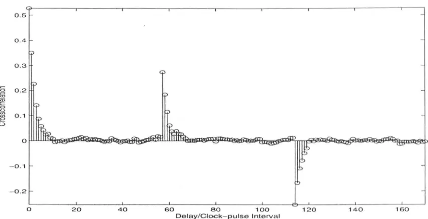
processes, automotive suspensions and tyres. In Chapter 3, the detection of the departure from linearity is considered. It is found that only signals based on maximum length sequences allow the detection of such characteristics due to the coherent patterns formed in the crosscorrelation function. These patterns are caused by the shift-and-add and shift-and-subtract properties of these signals. After detecting the departure from linearity, the 'combined' linear dynamics of the system are identified in Chapter 4 using correlation analysis, and various models and estimators (such as the autoregressive (ARX) and the autoregressive moving average (ARMAX) models, and the Estimator for Linear Systems (ELiS» in the System Identification Toolbox and the Frequency Domain System Identification Toolbox in MATLAB. It is concluded that while signals based on maximum length sequences should be used for the detection of the departure from linearity, their corresponding inverse-repeat signals should be used for estimating the linear dynamics. This is because the use of inverse-repeat signals eliminates the effects of even order nonlinearities, hence resulting in higher accuracy in the estimates obtained.

(19)

1 Introduction 7

In the thesis, the modelling of such processes using a neural network is also considered, and this is the main topic of Chapter 6. The network has an architecture which is based on, and modified from, the fully recurrent network. Such an architecture is referred to as 'semirecurrent' since only past values of the predictions of the network are fed back to the input layer. The performances of the two types of models (the Wiener model and the neural network model) are compared for different input signals and process dynamics. An experiment is conducted on a real process, namely an electronic nose. The input to the process is the chemical odour (acetone in this case) and this is controlled by a set of valves which determine if the odour could reach the metal oxide semiconductor (MOS) sensor. The output of the process is the voltage across the sensor. The direction-dependent characteristics of the electronic nose is caused by the different adsorption and desorption rates of the sensor. It is found that the neural network model works better in this case due to the process being predominantly first order and the input signal being binary. This is consistent with simulated results. However, the Wiener model provides a better match for an actual process when a multi sine input is used and the process is first order. Also, when the process is second order, it is found that only the Wiener model is capable of modelling the process.

(20)

1 Introduction ₈

The thesis then moves on to the topic of autotuning in Chapter 8. The autotuning of Smith predictors for processes with significant dead time is considered. The frequency response of the process is identified in closed-loop using a multi sine signal. Next, a parametric model is obtained using least squares. Tuning rules for robust control are suggested which relate the controller parameters to the process parameters. This reduces the problem of autotuning to that of a relatively simple task of process identification. Reduced order modelling for high order processes and for those with non-minimum phase is also studied. These processes can be modelled using a lower order model with dead time. An experiment was carried out using a hot-air flow device which proves that the performance of the Smith predictor with PI control is better than that either using the PI control alone, or using the Dahlin controller. This is indeed a very interesting result considering that the ratio of the dead time to the time constants of the process is in fact less than unity.

The final part of the thesis looks at the identification of Wiener-Hammer stein models. In Chapter 9, a new technique using linear interpolation in the frequency domain (shortened as LIFRED) is proposed for the identification of such a process with quadratic nonlinearity. The idea is based on the extraction of the symmetry properties of the Volterra kernel. This method, which makes use of multisine signals with no interharmonic distortion, has the advantages that only a single experiment is needed, and it is simple to use since no optimisation or recursive computations are required. Simulation examples are provided to illustrate the effectiveness of the technique, and its robustness in the presence of noise and input signal distortion. It is shown that despite the use of linear interpolation, the method works well even if the frequency response gain and phase curves could not be approximated by a straight line.

(21)

llntroduction 9

same frequencies as the input harmonics can be used in the estimation of the gain of the first linear subsystem (the one that precedes the nonlinearity). These are normally discarded in most estimation techniques due to the contributions of several different combination of the input frequencies falling on each of these estimation lines, and hence cannot be separated. However, these lines have a larger magnitude (due to the contribution of the linear term) and it is therefore advantageous to make full use of them in the estimation process, particularly since they are always present and could not be eliminated by signal design.

(22)

Chapter 2 Design of Pseudo-random Perturbation

Signals for System Identification

(23)

2.1 Abstract 11

2.1 Abstract

Pseudo-random signals have been widely used for the purpose of system identification. To identify a linear system or a nonlinear system with a Wiener structure, a binary signal is preferred as the signal power is maximised within constraints of the signal amplitude. Among the classes of pseudo-random binary signals, those based on maximum length sequences are the best known because of their ease of generation using feedback shift registers. However, it is less well known that there are several other classes of binary and near-binary signal with identical, or nearly identical, autocorrelation properties. An overview of these classes of signal is given and the design of a new MATLAB routine incorporating all these classes of signal (including the maximum length binary signal) is described. Three measures of signal quality are also reviewed. This chapter then goes on to consider the design of multi-level signals for the identification of nonlinear systems with the Hammerstein structure. Four measures related to the Vandermonde matrix of the system are used to evaluate the optimal signal levels and the number of occurrences of each of these levels.

2.2 Introduction

Periodic signals [1, 2] have been widely used in the field of system identification. These signals can be split into two main categories. The first is computer-optimised signals. Examples are multi sine (sum of harmonics) signals [3] and discrete interval binary signals [4] which can be generated using the MATLAB Frequency Domain System Identification Toolbox [51, and multi-level multi-harmonic signals [6].

(24)

2.2 Introduction 12

Appropriately chosen pseudo-random signals provide highly acceptable alternatives to multi sine signals in applications requiring uniform power in the frequency spectrum [4]. This is the most common requirement in practice. In many cases, the input transducer of a system can only cope with a small number of discrete amplitudes, resulting in a problem with the use of multisines, which effectively have an infinite number of levels. An additional advantage of binary signals is that, within constraints of the signal amplitude, the power injected into the process is maximised (or nearly maximised in the case of near-binary signals) which means that the effects of noise can be minimised . . This makes binary signals the preferred choice in the identification of linear systems. The only disadvantage of pseudo-random signals compared with multi sines is that non-uniform specifications in the frequency spectrum cannot be exactly met as their frequency spectrum is fixed.

MLB signals have periods N

=

2n - I (where n is an integer> I) [9], that is N

=

3, 7, IS, 31, 63, 127, 255, 511, 1023, 2047, etc. and can be easily generated in hardware using shift registers. The shape of the autocorrelation function approximates that of an impulse. For an MLB signal with levels ±1, the on-peak value of the autocorrelation is +1 and the off-peak value is -liN. However, as N increases, there are large gaps between successive periods [4]. This may pose a problem if an inflexible specification is given since the limited number of possible periods may result in the use of a signal with an excessively large value of N, so that the specified harmonics contain too little of the total signal power [4]. Fortunately, these gaps can be filled in by other classes of binary and near-binary signal such as quadratic residue binary (QRB), Hall binary (HAB) and Twin Prime binary (TPB) signals, which have identical autocorrelation properties to MLB signals, and with quadratic residue ternary (QRT) signals, which have almost identical autocorrelation functions [10]. It is therefore useful to design a new MATLAB routine to generate all these classes of signals, and this will be discussed in Section 2.3.

(25)

2.3 Design ola New MATLAB Routine 13

systems, such as the Wiener and Hammerstein structures. These structures have been widely investigated in the literature, for example in [11 - 16]. The use of pseudo-random binary signals for the identification of nonlinear systems is advocated in [17], and this is indeed true for nonlinear systems with the Wiener structure since the signal is a direct input to the linear subsystem [18]. However, binary signals do not sufficiently excite Hammerstein systems and this is shown in [19, 20] using quadratic Volterra filters. The design of multi-level signals for the optimum identification of nonlinear systems with the Hammerstein structure is considered in Section 2.4. Four measures are used to evaluate, in terms of obtaining the maximum accuracy in solving for the coefficients of the nonlinearity in the presence of noise, the quality of the Vandermonde matrix describing the system. It will be shown that the optimal signal in the above context is contradictory to the requirement of maximising the signal power within a specified signal amplitude.

2.3 Design of a New MAT LAB Routine

2.3.1 Generation of Maximum Length Binary Signals and the Design of

Related Functions

2.3.1.1 Generation of Maximum Length Binary Signals

(26)

2.3 Design of a New MATLAB Routine 14

(modulo-2) of degree 16 or less are given in [21] and the polynomials which are primitive are clearly indicated. Similar tables for degree 19 or less are given in [22]. An example of a primitive polynomial (modulo-2) for each n which satisfies 2::;; n::;; 100, and for n = 107 and 127 is listed in [23].

equation is in the delays introduced by the shift register [24]

:-c"D" Ee₂C,,_tD,,-t Ee₂".Ee₂_ctDEe₂Co = 0 (2.1)

Using the fact that modulo-2 addition is equivalent to modulo-2 subtraction, the feedback configuration [9] is given by

(2.2)

where X is the input signal to the shift register, DX is the sequence at the output of the

first stage of the register and so on, so that DnX is the sequence at the output of the last

stage of the n-stage register.

The MATLAB routine allows the user to specify a characteristic equation. If this is not irreducible and primitive, an error message is given. If no characteristic equation is specified, the default MLB signal is generated which makes use of the function mlbs [5] in the MATLAB Frequency Domain System Identification Toolbox.

2.3.1.2 Calculation of Resulting Shift due to Shift-and-add Property

The shift-and-add property [25, 26] states that when an MLB signal which is delayed by

a

is added to the same signal delayed by

p,

the resulting signal is the same signal

delayed by y. This property is unique to maximum length signals. For sequence levels 0

and 1

:-(2.3A)

(27)

(2.3B)

Thus terms with multiple products of inputs u can be replaced by terms with single lags in u [27]. These lags are dependent on the particular MLB signal used and are different for different MLB signals of the same period.

The MATLAB routine offers functions to calculate positions of the resulting lags for different shifts of the original signal, when two or three (shifted) signals are added together. The first signal is used as a reference and is not shifted. In the case of two signals added together, the second signal is delayed with respect to the first signal. If three signals are added together, the second and third signals are delayed with respect to the first signal. If an inverse-repeat signal is used, the routine allows only three signals to be added as the addition of two signals will not result in a shifted version of the original signal.

2.3.1.3 Measures of Rejection of Unsystematic Errors

When an MLB signal is used to estimate a system weighting function obtained by input-output crosscorrelation, there are errors introduced when nonlinearities that may be described by a Volterra functional series [28] are present [29]. Examples in the literature where these effects are investigated are given in [25, 30]. These errors can be classified into systematic and unsystematic errors. Unsystematic errors are dependent on the particular MLB signal used.

Unsystematic errors due to second order nonlinearities occur when

Si_J EB2 Si_K EB2 SI_I = 0 (2.4)

where i, J, K and I are integers. Similarly, those due to third order nonlinearities occur when

~JEB2~KEB2~LEB2~/=0

where L is also an integer.

(28)

If 0 ~ J < K < I in equation (2.4) and O~J<K<L<I in equation (2.5), two quantities Ro and R, can be defined as the upper bounds of I below which equations (2.4) and (2.5) respectively are not satisfied [29]. These measures can be used as a guide to the position of the nearest significant unsystematic error from the zero-lag position in the crosscorrelation function. Hence, for a particular signal period N, the signal with feedback connections resulting in the largest possible values of Ro and R, is preferred.

MLB signals with the greatest rejection of unsystematic errors and their corresponding values of Ro and RI are tabulated in [29] for 2 ~ n ~ 11. The values of Ro and RI are calculated and automatically displayed when the MATLAB routine is used to generate an MLB signal. If an inverse-repeat signal is generated, only the value of RI will be displayed since the effects of second order nonlinearities are eliminated.

2.3.2 Other Classes of Signal Available

The main objective of the new MATLAB routine is to generate the QRB, QRT, HAB and TPB signals, and their corresponding inverse-repeat signals.

QRB signals exist for N = 4k - I, where k is an integer and N is prime [9, 10], that is N =

3,7,11,19,23,31,43,47,59,67,71, 79, etc. The sequence {x,}, r = 1,2, ... ,Nis

formed from the rule

xr = + 1 if r is a square, modulo-N x, = -1 otherwise

XN = +1 or-I (2.6)

(29)

signal levels + 1, 0 and -1, the on-peak value of the autocorrelation is (N-l)/N and the off-peak value is -liN.

HAB signals exist for periods N

=

4~

+

27, where k is an integer and N is prime [10], that is N

=

31, 43, 127,223,283, 811, 1051, 1471, 1627, etc. A primitive root u of N is first chosen. The sequence is formed from the rule that

xr= +1 ifr ==

d,

modulo-N, where t == 0, 1 or 3 (modulo-6)

Xr = -1 otherwise (2.7)

A list of least primitive roots up to 4000 is given in [31]. For primes larger than 4000, a separate routine was written to find the least primitive roots and the results were incorporated into the MATLAB routine.

TPB signals exist for N = k (k+2), where k and k+2 are both primes [10), that is N == IS, 35, 143, 323, 899, 1763, 3599, 5183, etc. First QRB sequences are generated for both lengths k and k+2; these sequences are denoted by {ar} and {br } respectively. The TPB

sequence {xr } is then defined by

Xr

=

a,br for r "¢ 0, modulo-k or modulo-(k+2)

Xr= + 1 if r == 0 modulo-(k+2)

Xr

=

-1 if r

=

0 modulo-k, but r ~ 0 modulo-(k+ 2) (2.8)

An alternative method to generate

a

TPB sequence is to make use of a common primitive root u of k and (k+2) [10]. A difference set is formed, modulo-k(k+2), from

1 2 (pl-3)/2.

, u, U , ••• , u , 0, (k

+

2),2(k

+ 2), ... , (p -

l)(k

+ 2)

A TPB sequence is then derived from the difference set.

The first method is used in the MATLAB routine as it allows the shared use of the function to generate QRB signals.

The MATLAB routine can generate signals up to a length of 50000. This length is limited

(30)

Two harmonic specifications are available. All the signals above have all harmonics

present. Signals with only odd harmonics present can be generated by inverting every

other element of the sequence on which the signal is based, so producing an

inverse-repeat signal of period 2N. These signals have the property that the effects of odd and

even nonlinearities can be separated at the system output. Additionally, the effects of

even order nonlinearities are eliminated in the input-output crosscorrelation function.

2.3.3 Other Functions Available

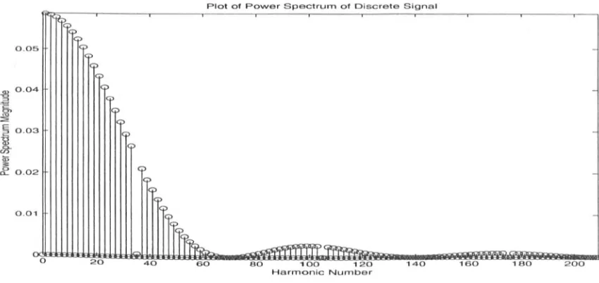
The program allows the user to plot graphs of the signal, its discrete Fourier transform,

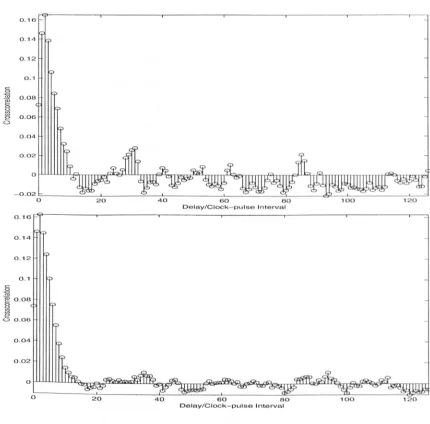
power spectrum and autocorrelation function. Examples are given in Figures 2.1 to 2.4

for a TPB signal oflength 35. From Figure 2.2, it can be seen that the signal contains all

harmonics, and the spectrum is flat except at dc. In Figure 2.3, the power spectrum for

three periods is plotted and this has a (Si: x

J

envelope. The on-peak value of the

autocorrelation is

+

I (at zero delay) and the off-peak value is -1135. Examples are given

in Figures 2.5 to 2.8 for the corresponding inverse-repeat signal. From Figure 2.6, the

signal contains only odd harmonics, and the spectrum is flat except at harmonic 35,

which is the Nyquist frequency. The autocorrelation function has a value of

+

I at zero

delay, -1 at a delay of 35 clock-pulse intervals, + 1/35 at odd numbers of delay/

clock-pulse interval and -1/35 at even numbers of delay/clock-pulse interval.

Plato' s lonol Lovels

I - -

-

r - - r - -

-0.6

0.6

0.4

0.2

] ~ 0 en -0.2 -0.4 -0.6

-0.6

- ' - - ' - - -

-

'--- 1

0 ₅ ₁₀

15 20 25 30 35

Nurnbor of Clock Pulses

(31)

2.3 Design o/a New MATLAR Routine

6 Plot of Discrete Fourier Transform of Discrete Signal

5

'I>"

5 10 15 20 25

Harmonic Number

Figure 2.2. Discrete Fourier transfonn of a TPB signal of length 35.

0.05

Cl) 0.04

i

~

i

0.03 l;;

~ 0.02

0.01

o 10

j) j)

i'

20

Plot of Power Spectrum of Discrete Signal

30 40 00 60 70

Harmonic Number

Figure 2.3. Power spectrum of a TPB signal oflength 35.

Plot of Autocorrelation Function of Signal

0.9

O.S

0.7

oS

.5ll

0.6

i

0.5 -< 0.4 0.3

0.2

0.1

0

0 5 10 15 20 25

Delay/CloCk-pulse I ntarval

Figure 2.4. Autocorrelation function of a TPB signal oflength 35.

so

19

-30

90 100

(32)

Plot of Signal Levels

- - r-:-- r - r-- -

-

r

-0.8

0.6

0.4 0.2

~ _o

~

en -0.2

-0.4 -0.6

-0.8

- 1 L - ' - - - - ' - - - - ~ ' - - - - ~ L - l . . .

-o 10 20 30 40 50 60 7 0

Number of Clock Pulses

Figure 2.5. Inverse-repeat TPB signal of length 70.

Plot of Discrete FourIer Transform of Discrete Signal

2

0

8

6

4

2 _'i'

o 10 20 30 40 50 60

Hannonlc Number

Figure 2.6. Discrete Fourier transfonn of an inverse-repeat TPB signal of length 70.

0.05

-§ 0.04

'

6-::!l!1 !l! 0.03

I

j

0.02

0.01

o 20

G> i' (i' i> i' 40

Plot of Power Spectrum of Discrete Signal

i>

IIri~

₆₀ ₈₀ ₁₀₀ ₁₂₀ ₁₄₀ ₁₆₀

Harmonic Number

Figure 2.7. Power spectrum of an inverse-repeat TPB signal oflength 70.

[image:32.529.75.500.528.729.2]

(33)

2.3 Design of a New MA TLAB Routine 21

Plot of Autocorrelation Function at Signal

O.B

0.6 .. 0.4

c:: 0.2

i

j

0

ex: -0.2 -0.4

-0.6

- O.B

-1ob---~,0~---2~0---~3~0--~---J40---~5~0~----~670---=70 Delay/Clock-pulse Interval

Figure 2.8. Autocorrelation function of an inverse-repeat TPB signal oflength 70.

The routine also incorporates functions to calculate different measures of signal quality.

The Performance Index for Perturbation Signals (PIPS) [4] is given by

PIPS =

200~urm

/

- Umean

2

%

u max -umin

(2.9)

where Unns is the rms value of the signal, Umean is the mean value of the signal, and Umax

and Umin are the maximum and minimum values ofthe signal respectively.

It is used to evaluate the performance of a signal in maximising the power in specified

harmonics within amplitude constraints. This is important since the signal amplitude

should be small enough to negate the effects of nonlinearities and the power contained

in the specified harmonics should be large enough to negate the effects of noise. In the

case of periodic signals, PIPS can be expressed in terms of the harmonic content of ti, so

that

N-i 200

IIU(k)1

2

PIPS= k=i %

N(umax - umin)

(34)

2.3 Design of a New MATLAB Routine

22

where U(k) is the discrete Fourier transform (DFT) magnitude of the kth harmonic of

u(t}.

An important advantage of PIPS is that it is independent of the signal mean and amplitude, thus making it more useful and versatile than other measures such as the Peak Factor, Crest Factor and Form Factor, which were originally used to quantify sine wave distortions. These measures have an additional disadvantage of being defined differently by different authors. A further advantage of PIPS is that it is 0% for a signal with the worst possible performance and 100% for a signal with the best possible performance. A pseudo-random binary signal has a PIPS of

100~1

-

~2

% while a

QRT signal has a PIPS of

100~1

-

~

% [4]. These tend to 100% as N increases. It should be noted that a binary signal in which the two levels have an equal duration or number of occurrences has a PIPS of 100% [4] and this is a great advantage over multi-level signals.

PIPS can be modified to suit particular applications and the derivation thus obtained is designated PIPS(Effective) or PIPSE [4], which is given by

R

200

I,1c'u(k)1

2

PIPSE = k=1 %

(umax - Umin)

R<NI2 (2.11 )

where IC'u(k}12 is the power of the kth harmonic of u(t} and the first R nonzero harmonics are specified for the identification. For a pseudo-random binary signal, PIPSE IS

100 2(N +2 I}

~

(Sin

1tk I N)2

k % whereas for a QRT signal, PIPSE IS

N k=1 rck / N

(35)

The use of PIPS and PIPSE alone as a measure of signal quality would not take into account the possibility that the power contained in one of the specified harmonics is low, and hence result in an inaccurate estimation of the frequency response at that particular frequency. A frequency domain measure of signal quality is then used which is the effective minimum ratio between the actual harmonic amplitude and the specified harmonic amplitude at any of the specified harmonics, EMINE [4]. This is defined as

1c',,(k)1

EMINE

=

100 minimum

--;========%

k=I.2 •..• R ~

ilc',,(k)1

2

R k=1

R<N12 (2.12)

EMINE is also independent of the signal mean and amplitude, and has a value of 0% for a signal with the worst possible performance and 100% for a signal with the best possible performance. For both pseudo-random binary signals and QRT signals, the Rth

(sin 1tR /

N)

harmonic has the least power, so that EMINE is 100 'TtR / N % [4].

!

i

(Sin rck /

N)2

R k=1 'Ttk / N

(36)

Signal type R PIPSE (%) EMINE (%)

PRB 15 48.4 98.6

PRB 30 66.9 94.0

PRB 63 87.9 73.0

QRT 15 48.2 98.6

QRT 30 66.6 94.0

QRT 63 87.5 73.0

Table 2.1. PIPSE and EMINE for different values of R using a pseudo-random binary (PRB) signal and a QRT signal, both withN= 127.

2.3.4 List of Functions

The MATLAB routine has a script file and 29 function files. The routine is started by running the script file and it will call other function files as necessary. A brief description of the purpose of the script file and all the function files is given below. The script file, prs-perturbation, is listed first followed by the function files in alphabetical order. A complete program is given in the Appendix.

Script file :

prs-perturbation

Function files:

autocorrelation autocorrelation-p1ot

calculate __ ~AfIN~

calculate __ PIPS calculate __ PIPS~

To generate binary and ternary pseudo-random signals. These signals can have either all harmonics present or only odd harmonics present.

To calculate the periodic autocorrelation of a signal.

To display the autocorrelation function graphically (and numerically if required).

(37)

DFT-plot

inverseJepeat

MLB

power-plot

prime

To calculate the limit in which unsystematic errors due to second order nonlinearities cannot be eliminated when an MLB signal is used to estimate the system weighting function (see Section 2.3.1.3).

To calculate the limit in which unsystematic errors due to third order nonlinearities cannot be eliminated when an MLB signal is used to estimate the system weighting function (see Section 2.3.1.3).

To calculate the discrete Fourier transform magnitude and present it graphically.

To generate HAB signals.

To check whether a HAB signal is present for a particular length.

To generate an repeat signal from a non inverse-repeat signal.

To generate MLB signals. The characteristic equation can be specified by the user. Otherwise, the function mlbs in the MATLAB Frequency Domain System Identification Toolbox is used to generate a 'default' MLB signal.

To check whether an MLB signal is present for a particular length.

To check if the characteristic equation of a shift register is irreducible and primitive. In other words, this checks if the signal generated by the shift register will be a maximum length signal (an MLB signal in this case). (This was discussed in Section 2.3.1.1.)

To generate an MLB signal when a characteristic equation is specified.

To calculate the power spectrum and display the results graphically (and numerically ifrequired).

(38)

2.3 Design of a New MATLAB Routine

26

prs_alCharmonics

sequence-plot signaCdisplay

TPB

To generate binary and ternary pseudo-random signals with all harmonics present.

To generate binary and ternary pseudo-random signals with only odd harmonics present.

To generate QRB signals.

To check whether a QRB signal is present for a particular length.

To generate QRT signals.

To check whether a QRT signal is present for a particular length.

To calculate the shift in the resulting signal when an MLB signal is shifted by a particular delay and then added on to the original (non shifted) signal.

To plot the generated signal.

To display the generated signal, its discrete Fourier transform, power spectrum and autocorrelation function by calling the functions sequenceJJlot, DFT-plot, powerJJlot

and autocorrelationJJlot respectively. It also allows the user to save the data relating to the generated signal in an external file.

To calculate the shift in the resulting signal when two MLB signals which are shifted by two different values of delay are added on to the original (non shifted) signal.

To generate TPB signals.

To check whether a TPB signal is present for a particular signal.

A routine to find the least primitive root for any given prime number, primitiveJoot,

(39)

2.4 Extension to Multi-level Pseudo-random Signals

27 2.4 Extension to Multi-level Pseudo-random Signals

2.4.1 Introduction to Nonlinear System Identification

The identification of nonlinear structures such as the Wiener and Hammerstein models using pseudo-random signals is investigated in [18]. It is shown that for the Wiener model in which a dynamic linear subsystem precedes an instantaneous nonlinearity, the performance of the signal measured using PIPS is the same as for a linear system. It is concluded in [18] that a binary signal with a PIPS of 100% will give the best performance with the Wiener model.

More complicated analysis is needed for the Hammerstein model, in which a dynamic linear subsystem succeeds an instantaneous nonlinearity. Such a structure with quadratic nonlinearity is considered in [18]. In this case, a perturbation signal with at least three levels is needed to identify the linear and nonlinear parts of the system. This is because a binary signal will produce a constant at the output of the quadratic nonlinearity. It is also shown in [18] that it is desirable for the signal to have even harmonics suppressed and its odd harmonics uniform. In addition, the square of the signal should have its odd harmonics suppressed and its even harmonics, apart from the zero harmonic, uniform. This is because the square of the signal will be an input to a linear subsystem, and hence the perfonnance criteria should be applied to it as well. The theory can be extended to Hammerstein models with a higher order of nonlinearity. To identify a system with ND -1 order of nonlinearity, the signal must have at least ND levels [32]. The optimum signal levels were found in [32] by minimising the condition number of the associated Vandermonde matrix [33].

(40)

2.4 Extension to Multi-level Pseudo-random Signals 28

2.4.2 Properties of Multi-level Signals

Multi-level signals u(i) may be obtained from maximum length sequences s(i) generated in the Galois field GF(q). Such a sequence has a period N

=

qn -I and can be divided into q-I subperiods. Each period of the signal contains qn-I occurrences of each elements, except element 0 which occurs only qn-I_I times.

2.4.2.1 Three-level Signals

Several properties of three-level maximum length sequences generated from GF(3) are given in [35, 36]. Examples of shift register feedback connections resulting in such a signal for 2 ~ n ~ 7 are given in [35] and these were derived from a list of primitive polynomials tabulated in [37]. Since the signal can be divided into two subperiods, it is

therefore an inverse-repeat signal.

F or such a signal u(i), the magnitudes of the harmonics are given in [18] by IU(k~ = 2 X 3(n-I)/2 k odd

IU(k~

=

0 keven (2.13)

PIPS is IOO~2(N

+

I) / 3N%, which tends to 81.6% as N increases [18]. In the

identification of Hammerstein models with ND - I = 2, the magnitudes of the harmonics of the square of the signal v(i) are of importance as the signal v(i) = u(i)2 will be an input to the linear subsystem. The magnitudes of these harmonics are given by

IV(k~ = 2 x 3n-1 k= rN

IV(k)1

=

2 x 3(n-2)/2

IV(k~ = 0

keven'# rN

kodd (2.14)

(41)

2.4.2.2 Four-level Signals

Four-level maximum length sequences based on GF(4) are considered in [38,39]. If the elements (0, I, 2, 3) of the sequence are mapped into signal levels (ut, U2, U3, U4), the mean value M is given in [39] by

M = U\ +u2 +u3 +u4 + U2 +u3 +u4 -3u)

4 4(4111 -I)

The normalised autocorrelation function is given by

2 2 2 2 2 2 2 3 2

R(O)=U) +u2 +u3 +u4 +u2 +u3 +u4 - u\

4 4(4'" -I)

R(k) = (u\ +u2 +u3 +U4 )2

+

(u\ +u2 +u3 +U4 )2 -16u\2

16 16(4111 -1)

where k is not an integer multiple of N/3.

(2.15)

(2.16)

(2.17)

(2.18)

If we consider equal spacing between the signal levels by taking u\ = C, U2

=

C

+

A,

U3

=

C + 2A, U4

=

C

+

3A as was done in [39], equations (2.17) and (2.18) can be simplified to

R(N) = R(2N) = C2 + 12AC + I1A2 ( 4111 )

3 3 4 4111 - 1 (2.19)

R(k) = C2 + 12AC + 9A2 ( 4111 )

4 4'" - I (2.20)

Since equation (2.19) cannot be made equal to equation (2.20) (unless A

=

0, resulting in a constant signal), the autocorrelation function is not primitive and the harmonics are

not uniform in magnitude. Also, inverting every other member of the signal does not produce an inverse-repeat signal with uniform odd harmonics.

(42)

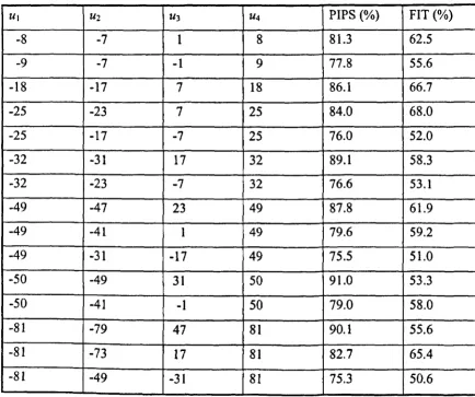
the separation of levels very far from being equal, thus greatly limiting its usefulness in a perturbation test. The equality of spacing between the levels can be measured using its FIT value. For a signal with equal spacing, the signal levels are

F or a particular four-level signal, the error term is defined as

error

=

u - u + 4 \ + u - u _ 4 \

( u -u ) ( u -u )

2 \ 3 3 4 3

and FIT is then defined as

FIT =

100(

1 - error)% U4 -u\

(2.21)

(2.22)

(2.23)

Some mapping levels for four-level signals with uniform harmonics (except at dc) are given in Table 2.2, together with their values of PIPS (defined in (2.10)) and FIT.

u\ U2 U3 U4 PIPS (%) FIT (%)

-8 -7 1 8 81.3 62.5

-9 -7 -1 9 77.8 55.6

-18 -17 7 18 86.1 66.7

-25 -23 7 25 84.0 68.0

-25 -17 -7 25 76.0 52.0

-32 -31 17 32 89.l 58.3

-32 -23 -7 32 76.6 53.1

-49 -47 23 49 87.8 61.9

-49 -41 1 49 79.6 59.2

-49 -31 -17 49 75.5 51.0

-50 -49 31 50 91.0 53.3

-50 -41 -1 50 79.0 58.0

-81 -79 47 81 90.1 55.6

-81 -73 17 81 82.7 65.4

[image:42.547.77.511.357.720.2]

-81 -49 -31 81 75.3 50.6

(43)

2.4.2.3 Five-level Signals

For pseudo-random sequences u(i) obtained from GF(5), the mapping of the sequence

elements into signal levels which result in uniform harmonics can be written as

UI =0

U2 = -us

=

a

(2.24)

When a > I and b = I, u(i) has five levels. Typically, a = 2 since this gives equal spacing between the levels. The magnitude of the harmonics are then given by

IU(k~ = 4.47 x S(n-I)/2

IU(k)1

=

0

kodd

keven

The closer a is to unity, the larger the value of PIPS.

(2.25)

The field elements can also be mapped such that the resulting signal is three-level by making a

=

0 and b = 1, or a = b = 1. In the former case,

IU(k)1 = 2 X S(n-O/2

IU(k~ = 0

In the latter case

IU(k)1

=

2.83 x S(n-I)/2 IU(k)1

=

0

kodd

keven (2.26)

kodd

keven (2.27)

(44)

2.4.3 Design of Multi-level Signals for the Identification of

Hammerstein Models

For the identification of a nonlinear system with the Hammerstein structure, a multi-level perturbation signal u is required. The signal must have at least ND different levels if the order of the nonlinearity is ND - 1. For the present, assume that every level has the same number of occurrences. Without loss of generality it may also be assumed that U1 >u2 > ••• >UND , and that u1 =1 and UND =-1. Despite the fact that intuition may suggest that the levels be equally spaced, this may not be the optimal solution.

To fonnulate the problem, the output of the nonlinear system Y is expressed as a function of the input u.

Then the output of the nonlinearity at each signalleve1 is given by

Yl u, ND-l U_tNJ)-2

..

Y2

ND-l NJ)-2 u2 u2

..

=

YNJ)-l _{U ND - 1}ND-l U ND - 2 Nf)-t

..

YNo UN/) ND-I U_NDND-2

..

UN/J-l

t U No - 2 t

..

u1 1

ND-l ND-2 _u

2 1

u₂ u₂

..

where

uNn - t Nn-I U No

-2

No-l

..

UNJ)-l 1 ND-l _ND-2

U_ND 1

u_ND u_ND

..

Equation (2.29) may be written as y= V_N (u)a

D

hence

U_t a(

u₂ 1 a 2

U ND - 1 1 aNJ)-1 U

ND 1 aND

is the Vandennonde matrix of

(2.28)

(2.29)

u₁

u₂

U No - 1

U ND

(2.30)

(45)

There are several ways to select the optimal values of u. These are given below:

(a) In the context of a measurement problem, errors occur in the measurements y, and

the requirement is to minimise the sensitivity of the solution to these errors. The sensitivity matrix is

da (

)-1

- = V_N (u)

dy D

(2.32)

and it is therefore required to minimise the sum of all sensitivities

~~I(VND(U)rl·jl

, J

(2.33)

(b) It is also possible to minimise the greatest sensitivity given by

(2.34)

( c) In the context of a least-squares polynomial fitting problem, errors occur in y and the effect of these errors is minimised by minimising

(2.35) (d) The problem can also be treated as a matrix inversion problem where numerical errors occur in the inversion of V_N (u). In this case, the quantity to minimise is the

D

2-norm of the condition number of v'N (u) I)

(2.36) as was done in [32]. This is defined as

(2.37)

where

A.

represents the singular values of a matrix.

These four measures all give the same result when

ND

= 3. In this case

(2.38)

(46)

1 I 1

(u, -u2)(u, -u_{J )} _{(u2 -U3)(U2 -u\)} (u) _-UI)(U3-u₂₎

(VND(U)r' = U2 +u3 uJ +U, ul +u2

(ul - U2)(UI - u3) (u2 - u:J(u2 - ul) (u₃-u\)(u₃-u2 )

U2U3 U3U\ U\U2

(u_l_{-U2)(UI -u3)} _(u_{2 - U3)(U2 -} _u_l) (u_{3 -} u_{l)( U3 - U2 )}

1 1 1

-2(I-u_2} l-u₂2 2(1 +U2 ) I

0 1 (2.39)

=

-2 2

u2 I U2

2(1-u₂₎ l-u₂2 2(1 _+U2)

In this case all four requirements are satisfied when U2

=

0 which results in

[

0.5 -1 0.5]

(VN/) (u)r

=

00.5 0 0.5 1 0

(2.40)

The four measures do not, however, give the same results when ND > 3. These are tabulated in Table 2.3 for the cases when ND

=

4 and 5. Methods (a) to (d) correspond to minimising the quantities given in (2.33) to (2.36) respectively.

ND Method U2 U3 U4

4 a 0.425 -0.425

4 b 0.575 -0.575

4 c 0.545 -0.545

4 d 0.520 -0.520

'5 _a _0.655 ₀ _-0.655

5 b 0.840 0 -0.840

5 c 0.745 0 -0.745

5 d 0.725 0 -0.725

(47)

The results for ND

=

3,4, and 5 all have a symmetry of the fonn

r

=

1, 2, ... (2.41)

Also, as the only known four-level signals with ideal hannonics are very asymmetric, the above results indicate that they are not likely to be suitable for this application.

The above analysis needs to be modified if a nonlinearity of order ND - r (where r #:- 1) needs to be identified instead, and if some or all of the signal levels occur more than once. In the first case, the number of columns of the Vandennonde matrix is reduced, while in the second case, the number of rows of the matrix is increased. This modification does not change the basic solution of the problem except that the measures given in methods (a) to (d) are applied to a modified version of the Vandennonde matrix

Vm.

Due to the fact that the modified matrix is no longer a square matrix, it is now required to minimise

(a)

~~I((vm(ul'vm(u)r'vm(ul'LI

(b)

lIlj'x(

mr(I((Vm(ul'vm(u)r' Vm(u)'LI))

(c)

II(Vm(ufVm(u)t Vm(ufll

(d) cond₂

(Vm(u)TVm(u»)

(2.42)

(2.43)

(2.44) (2.45)

When either a four-level or a five-level signal is used to identify a quadratic nonlinearity, all four requirements are satisfied by the same degenerate case for which

U2

=

U3

=

U4

=

O. Results obtained when a five-level signal is used to identify a cubic

nonlinearity are given in Table 2.4. Here, methods (a) to (d) correspond to minimising (2.42) to (2.45) respectively.