University of Warwick institutional repository:
http://go.warwick.ac.uk/wrap
This paper is made available online in accordance with
publisher policies. Please scroll down to view the document
itself. Please refer to the repository record for this item and our
policy information available from the repository home page for
further information.
To see the final version of this paper please visit the publisher’s website.
Access to the published version may require a subscription.
Author(s): Tappert, C.; Gaensicke, B. T.; Schmidtobreick, L.; Ribeiro, T.
Article Title: Accretion in the detached post-common-envelope
binary LTT 560
Year of publication: 2011
Link to published article:
http://dx.doi.org/10.1051/0004-6361/201116436
DOI:10.1051/0004-6361/201116436
c
ESO 2011
Astrophysics
&
Accretion in the detached post-common-envelope binary LTT 560
C. Tappert
1, B. T. Gänsicke
2, L. Schmidtobreick
3, and T. Ribeiro
41 Departamento de Física y Astrofísica, Universidad de Valparaíso, Av. Gran Bretaña 1111, Valparaíso, Chile
e-mail:[email protected]
2 Department of Physics, University of Warwick, Coventry CV4 7AL, UK
e-mail:[email protected]
3 European Southern Observatory, Casilla 19001, Santiago 19, Chile e-mail:[email protected]
4 Departamento de Física, Universidade Federal de Santa Catarina, Campus Trindade, 88040-900 Florianópolis, SC, Brazil e-mail:[email protected]
Received 4 January 2011/Accepted 11 June 2011
ABSTRACT
In a previous study, we found that the detached post-common-envelope binary LTT 560 displays an Hαemission line consisting of two anti-phased components. While one of them was clearly caused by stellar activity from the secondary late-type main-sequence star, our analysis indicated that the white dwarf primary star is potentially the origin of the second component. However, the low resolution of the data means that our interpretation remains ambiguous. We here use time-series UVES data to compare the radial velocities of the Hαemission components to those of metal absorption lines from the primary and secondary stars. We find that the weaker component most certainly originates in the white dwarf and is probably caused by accretion. An abundance analysis of the white dwarf spectrum yields accretion rates that are consistent with mass loss from the secondary due to a stellar wind. The second and stronger Hαcomponent is attributed to stellar activity on the secondary star. An active secondary is likely to be present because of the occurrence of a flare in our time-resolved spectroscopy. Furthermore, Roche tomography indicates that a significant area of the secondary star on its leading side and close to the first Lagrange point is covered by star spots. Finally, we derive the parameters for the system and place it in an evolutionary context. We find that the white dwarf is a very slow rotator, suggesting that it has had an angular-momentum evolution similar to that of field white dwarfs. We predict that LTT 560 will begin mass transfer via Roche-lobe overflow in∼3.5 Gyr, and conclude that the system is representative of the progenitors of the current population of cataclysmic variables. It will most likely evolve to become an SU UMa type dwarf nova.
Key words.binaries: close – stars: late-type – white dwarfs – stars: individual: LTT 560 – novae, cataclysmic variables
1. Introduction
Cataclysmic variables (CVs) are thought to form from detached white dwarf (WD)/main-sequence star (MS) binaries that have experienced a common-envelope (CE) phase (e.g., Taam & Ricker 2010;Webbink 2008). In these “post-common-envelope binaries” (PCEBs), the white dwarf represents the more mas-sive component in the system and is therefore called the pri-mary, while the usually late-type (K–M) main-sequence star is known as the secondary. After the end of the CE phase, angular-momentum loss due to magnetic braking and/or gravi-tational radiation continues to decrease the separation between the two stars. This eventually brings the secondary’s Roche lobe into contact with the stellar surface, thus initiating stable mass-transfer via Roche-lobe overflow and the semi-detached CV phase (Ritter 2008, and references therein).
There is growing evidence that the accretion of material from the secondary star does not start with Roche-lobe over-flow. The discovery of so-called “low accretion rate polars” (Schwope et al. 2002), which are likely progenitors of magnetic CVs (Schmidt et al. 2005,2007), and the detection of metal ab-sorption lines in the UV spectra of non-magnetic PCEBs (e.g.,
Kawka et al. 2008), indicate that wind accretion from the active Based on observations made at ESO telescopes (079.D-0276).
chromosphere of the secondary star is a common phenomenon in detached, short-period, WD/MS binaries.
Tappert et al.(2007, hereafter Paper I) found the Hα emis-sion line in the detached PCEB LTT 560 to be a combination of two components. The radial velocity variations in the stronger Hα component agree well with those shown by the TiO ab-sorption, and was thus identified as originating in the secondary star. The radial velocities of the weaker component showed an – within the errors – anti-phased behaviour with respect to the sec-ondary star exhibiting a lower amplitude, and therefore had to be produced on the side of the centre-of-mass opposite to the sec-ondary. However, the low spectral resolution of the data, and the contamination of the white-dwarf Balmer absorption lines with emission cores from the secondary, impeded velocity measure-ments of other, unambiguously intrinsic, spectral features from the white dwarf. Thus, the true origin of the weak emission com-ponent remained unresolved. The low temperature of the white dwarf in LTT 560 (T ∼7500 K, Paper I) and the evidence of on-going accretion imply that there is a high probability that there are narrow metal absorption lines in the white-dwarf spectrum (Zuckerman et al. 2003). The radial velocity curve of such lines should be undisturbed and thus faithfully track the motion of the white dwarf, motivating the high-resolution study presented in this paper.
A&A 532, A129 (2011)
2. Observations and data reduction
LTT 560 was observed on August 16, 2007 using UVES on UT1 (ANTU) at ESO Paranal. A total of 38 Echelle spec-tra was taken over 7.3 h in one blue (3260−4528 Å) and two red (5681−7519 Å, 7661−9439 Å, hereafter “lower” and “up-per” red spectrum, respectively) spectral ranges, with resolv-ing power∼70 000. The exposure time per spectrum was 600 s, which corresponds to roughly 0.05 orbital cycles. The sequence of time-resolved spectra had to be interrupted for about 45 min when the object was close to the zenith, where the VLT cannot observe.
The data reduction was performed using Gasgano and the UVES pipeline (version 3.9.0) in a step-by-step mode. This included bias and flat correction, wavelength calibration with a ThAr lamp, and flux calibration using the standard star LTT 7987. The response function proved rather unsatisfac-tory, with the flux-calibrated spectra still containing several “or-der wriggles”. However, since this bears no relevance to the work described in this paper, we did not attempt to resolve this issue.
3. Results
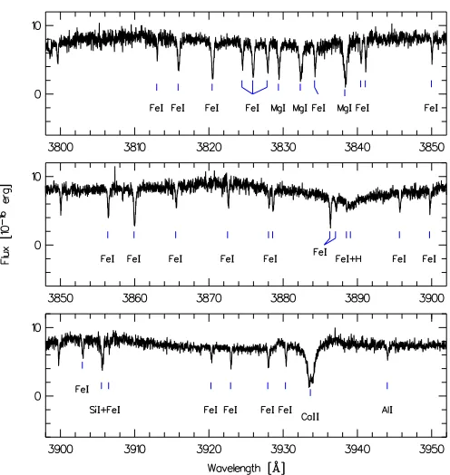
In Figs.1and2, we present selected wavelength ranges of the av-eraged blue and red spectra. For the computation of both spectra, the individual data were corrected for the motion of the respec-tive components based on the radial velocity parameters derived in Sect.3.1. Thus, Fig.1 shows the blue spectrum in the rest frame of the white dwarf, while Fig.2gives the red spectra in the rest frame of the late M dwarf. Absorption features of both stellar components were identified using the ILLSS catalogue (Coluzzi 1999).
The two red spectra are dominated by the features of the sec-ondary star, which are mainly molecular TiO bands, but also sev-eral atomic absorption lines such as Ca Iλ7326 (in the “lower” red spectrum), the Na Iλλ8183/8194 doublet, K I, Fe I, Ti I, and Ca II (in the “upper” red spectrum). As shown inPaper I, the red spectrum is consistent with an M5−6V secondary star. The blue portion of the spectra presents a plethora of narrow metal absorp-tion lines: these are mostly of Fe I, but also Ni I, Si I, Mg I, Al I, Ca I, and Cr I can be identified. In addition, there are the broader lines of Ca II, and H I. In Sect.3.2, we use the absorption lines of the white dwarf to estimate the accretion rate.
3.1. Radial velocities
We recall that the main motivation of the present work was to determine the origin of the two Hαemission components. This can be achieved by calculating the parameters of their respective radial velocity variations
vr(t)=γ+Ksin[2π(t−T0)/Porb], (1)
and by comparing them to the corresponding parameters of in-trinsic stellar absorption features. We therefore measured the ra-dial velocities of the following lines and spectral regions:
(1) The two Hαemission components were fitted individually with a single Gaussian. For the calculation of the parame-ters, we excluded the data close to superior and inferior con-junction, when both components merge.
[image:3.595.309.557.71.333.2](2) By fitting single Gaussians again, the velocities for 29 metal absorption lines in the blue spectral range (in the major-ity Fe I) were measured, and the fitting of sine functions according to Eq. (1) yielded the corresponding parameters.
Fig. 1.Selected ranges of the blue spectrum with line identifications. This average spectrum has been produced by combining 38 individual spectra that had each been corrected for the radial velocity variations of the white dwarf.
Fig. 2.Selected ranges of the average red spectra. The respective indi-vidual spectra have been corrected for the radial velocities of the sec-ondary star. The spectra are not corrected for telluric contamination. Indicated are the Hα emission line, the spectral range that has been used for the cross-correlation, and the absorption lines that could be unambiguously identified.
The sample was subsequently restricted to 16 curves with a standard deviation<0.5 km s−1 in γ to provide average parameters.
(3) The Na I lines were also measured with single Gaussian functions. An attempt to fit both lines simultaneously with two Gaussians at a fixed separation was unsuccessful be-cause of the irregular and variable continuum.
(4) Cross-correlation was performed for the spectral ranges 3810−3870 Å (containing several narrow absorption lines) and 7000−7200 Å (including three strong TiO absorption
[image:3.595.308.555.390.584.2]Table 1.Radial velocity parameters.
Feature K γ ϕ
[km s−1] [km s−1] [orbits] HαMSa 231.50±0.51 35.01±0.46 −0.00271(65) Na Iλ8183 233.72±0.33 35.59±0.24 0.00011(24) Na Iλ8195 228.92±0.29 37.96±0.22 −0.00019(22) TiO cc+λ0b 231.17±0.19 37.18±1.28 0.00009(14) HαWDc 72.70±0.15 55.69±0.14 0.50198(62) metalavd 72.63±0.88 54.24±0.88 0.5009(20)
metal cc+λ0e 72.62±0.16 55.20±0.74 0.50018(37)
Notes.(a)Broad Hαcomponent excluding conjunction spectra.(b)Kand ϕvia cross-correlation of the range 7000−7200 Å,γfrom the position of 15 red absorption lines.(c) Narrow Hαcomponent excluding con-junction spectra.(d)Average of the radial velocity parameters of 16 blue metal lines.(e)Kandϕvia cross-correlation of the range 3810−3870 Å, γaveraged from the positions of 31 metal lines.
bands). Lacking a proper radial velocity standard, the spec-tra were correlated to one spectrum of the data set of high signal-to-noise ratio (S/N). The resulting velocities were then fitted according to Eq. (1) withγset to 0. Subsequently, the individual spectra were corrected for the corresponding variation and averaged to yield high S/N spectra. Finally,
γwas determined by calculating the shift of spectral features with respect to their rest-frame wavelength in these average spectra. For the blue range, this shift was calculated as the average of the positions of 31 lines. For the red range, the Ca Iλ7326 line was used from the lower red spectrum and 12 lines from the upper red range.
Table1summarises the resulting parameters. The zero point of the orbital variationT0was set to the inferior conjunction of the TiO cross-correlation velocities, yielding an ephemeris
T0(HJD)=2 454 329.6840(29)+0.1475(29)E, (2)
whereE is the cycle number. The value for the orbital period was taken fromPaper I.
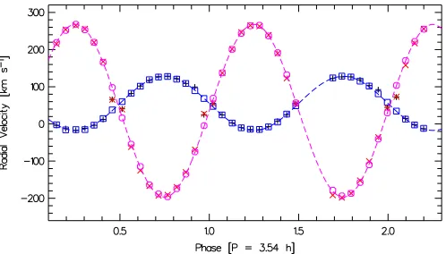
As can be seen in Table1, and is visualised in Fig.3, there is a close agreement between all parameters for the respective features of both the white dwarf and the secondary star. We may thus calculate the weighted averages for these parameters:
γWD =55.45(34) km s−1, KWD =72.66(11) km s−1, γMS=36.51(72) km s−1, KMS=231.22(95) km s−1.
With this, we derive the mass ratio
q=KWD/KMS=0.3143(13)
and the gravitational redshift of the white dwarf
vgr=γWD−γMS=18.94(80) km s−1.
These values are consistent with those determined inPaper I(q=
0.36(03),vgr = 25(09) km s−1), but represent a vast improve-ment in accuracy. Assuming a He-core and a CO-core white dwarf, and adopting the mass-radius relations fromPanei et al.
(2000) for a 10−5 M
hydrogen envelope, the gravitational red-shift corresponds toMwd =0.46±0.12MandMwd =0.44± 0.12M, respectively. The resulting updated system parameters (seePaper Ifor details) are summarised in Table2.
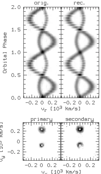
[image:4.595.44.288.98.201.2]In Fig.4, we show the trailed spectrum and the Doppler map that was computed using the fast maximum entropy algorithm of
Fig. 3.Radial velocities of several spectral features plotted against or-bital phase. The latter are presented in sequence, i.e. corresponding to their time of measurement. The plot shows the radial velocities for the broad and narrow Hαcomponents (marked by slanted and straight crosses, respectively), and the TiO and metal cross-correlation veloci-ties (circles and squares, resp.). The plot also includes the radial velocity curves calculated from the adapted average radial velocity parameters.
Table 2.System parameters of LTT 560.
WD Porb MWD MMS q i a
[h] [M] [M] [◦] [R]
He 3.54(7) 0.46(1) 0.146(4) 0.314(1) 63(2) 1.00(1) CO 3.54(7) 0.44(1) 0.139(4) 0.314(1) 65(2) 0.98(1)
Notes.Orbital period, masses, mass ratio, inclination, and binary sepa-ration for a He- and a CO-core white dwarf primary assuming a 10−5M
hydrogen envelope.
Spruit(1998). The flare data (Sect.3.3.1) were excluded, since Doppler tomography does not take into account non-orbital vari-ations. The resulting map represents a two-dimensional visual-isation of the emission distribution in velocity space (Marsh & Horne 1988). We note that the significant difference in theγ ve-locities caused by the gravitational redshift of the white dwarf requires the calculation of two maps with respective corrections. Consequently, the emission from the secondary star appears dis-torted in theγWD corrected map, and vice versa. We note that both the emission component from the white dwarf and the one from the secondary star in their respective “γrest frames” are symmetrically centred on the calculated positions of the stellar components, and that these two are the only Hαemitters in the system, i.e. no accretion stream or disc is visible in Hα.
3.2. The photospheric white dwarf spectrum
A&A 532, A129 (2011)
Fig. 4.Trailed spectra and Doppler maps. Thelower left plotpresents the Doppler map corrected forγWD, thelower right plotthe correspond-ing one corrected forγMS. The slanted and the straight cross mark the calculated positions of the stars, i.e.KWDandKMS, respectively. The up-per plots show the trailed spectra forγWD. Theleft spectrumrepresents the original data, theright spectrumis the reconstructed data from the Doppler map. The data are repeated for a second orbital cycle for clarity.
the individual abundances of these elements to achieve the clos-est fit to the observed line profiles (Fig.5). The abundances de-termined from this fit are reported in Table3, with typical un-certainties of 0.2 dex. Within these unun-certainties, the observed abundance pattern is broadly consistent with a solar element mixture at0.015 times the solar metal abundances (Asplund et al. 2009).
The relatively large abundances of metals in the photosphere of the white dwarf clearly indicate that it is accreting from its companion star. Doppler tomography rules out Roche-lobe over-flow, hence the origin of the accreted material is very likely to be the wind of the companion star. Assuming that the white dwarf photosphere is in a steady-state of accretion-diffusion, we can use the determined metal abundances to infer the accretion rate from
˙
M =qMWDX
τDXacc
, (3)
whereq is the mass fraction of the convection zone (in which the accreted material is mixed), τD is the diffusion timescale on which accreted metals drop out of the convection zone, and [X/H] and [X/H]acc are the abundances observed in the white dwarf atmosphere and in the accreted material, respec-tively (Dupuis et al. 1993; Koester & Wilken 2006). We as-sume that the white dwarf in LTT 560 accretes solar abundance material, and estimateq = −8.2 from the plots in Althaus & Benvenuto(1998).Koester & Wilken (2006) list the diffusion timescales for Ca, Mg, and Fe for a wide range of effective tem-peratures and surface gravities. We interpolate their Table2for
Fig. 5. The plethora of metal absorption lines in the average spectrum of the white dwarf in LTT 560 were fitted with TLUSTY/SYNSPEC models to determine the metal abundances in the white dwarf photo-sphere. The overplotted black line shows a model forTWD =7500 K, logg=7.75, and adopting the abundances listed in Table3.
TWD = 7500 K and logg = 7.75 to find τD(Ca) = 9400 yr, τD(Mg) = 9950 yr, and τD(Fe) = 7460 yr. Using the abun-dances of Ca, Mg, and Fe determined from our fits to the pho-tospheric metal lines (Table3), we obtain three independent es-timates of the accretion rate, ˙M =4.4×10⁻¹⁵ M
yr−1, 4.5× 10⁻¹⁵ M
yr−1, and ˙M =6.0×10⁻¹⁵ Myr−1. Within the uncer-tainties of our analysis, we conclude that the accretion rate onto the white dwarf is∼5×10⁻¹⁵M
yr−1.
[image:5.595.84.252.74.363.2]Table 3.Photospheric white dwarf abundances.
Element log[X/H]LTT5601 log[X/H]
2 ×solar3
Mg –6.2 –4.4 0.015
Al –7.6 –5.6 0.010
Si –6.2 –4.5 0.018
Ca –7.5 –5.7 0.015
Sc –10.9 –8.8 0.008
Mn –8.2 –6.6 0.018
Fe –6.3 –4.5 0.018
Co –8.8 –7.0 0.018
Ni –7.9 –5.8 0.007
Notes.Abundances determined from fitting TLUSTY/SYNSPEC
mod-els to the metal lines detected in the average UVES spectrum of LTT 560.
(1)Metal abundances relative to hydrogen, by number, for LTT 560. (2)As (1), but for the Sun.(3)The abundances in LTT 560 relative to
[image:6.595.59.274.99.205.2]those in the Sun.
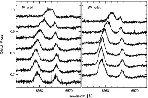
Fig. 6.Comparison of the two half orbits corresponding to the phase intervals 0.64−1.0 (left panel) and 1.64−2.0 (right) in Fig. 3. The Hαcomponent from the secondary star is clearly stronger at the start of the second panel, while the one from the white dwarf remains unchanged.
3.3. Activity 3.3.1. Flaring
In the second part of the second orbit covered by our data, the Hαcomponent from the late-type star is significantly enhanced from phases 1.7−1.9, i.e. immediately after the “zenith break” (Fig.6). In contrast, the white-dwarf Hα component remains constant. For a quantitative analysis, we measured the equiva-lent width of the secondary’s Hαcomponent as follows. First, we fitted single Gaussian functions to the line profile of the white-dwarf Hαcomponent in all spectra where this component was sufficiently isolated. Subsequently, all fits were subtracted from all spectra, and the quality of the subtraction was evaluated visu-ally. Eight fits were found to leave sufficiently negligible resid-uals. Finally, the equivalent widths of the secondary’s Hα com-ponent was measured in all eight sets of subtracted spectra.
For four spectra, none of the subtracted line profiles were of satisfactory quality, containing significant negative residu-als. Interestingly, three of those represent all the spectra in the phase interval 0.9−1.0, and one might speculate that at these phases (close to superior conjunction of the primary) the white-dwarf Hα component is affected by some sort of obscuration. Nevertheless, our coverage here is insufficient for an in-depth
Fig. 7.Equivalent widths of the Hαafter the emission component of the white dwarf had been subtracted from the spectrum. Open circles mark spectra where the subtraction left significant negative residuals.
analysis, and more data will be needed to confirm this apparent diminished strength of the white-dwarf Hαcomponent.
The average equivalent widths are plotted in Fig.7. The sec-ondary’s Hα component at second quadrature during the sec-ond observed orbit is clearly about 1.6 times stronger than dur-ing the first orbit. The observed maximum of this flare occurs at phase 1.7, but since the phase interval 1.5−1.7 was not cov-ered because of the zenith break it is possible that the real max-imum was reached before we recommenced observations. From phase 1.7 to the end of observations at phase 2.2, the strength of the Hαline had declined, but had not yet reached its “qui-escence” value at this point. We furthermore note that during the first observed orbit the equivalent width has a local maxi-mum at second quadrature, where it is about 1.4 times larger than at both observed “unflared” first quadratures (phases 0.25 and 1.25). This indicates that there is an active region on the leading side of the secondary star.
3.3.2. Roche tomography
To explore the secondary’s signatures of stellar activity, we used the method of Roche tomography (RT; Rutten & Dhillon 1994;Watson & Dhillon 2001), applying an image reconstruc-tion technique to obtain a brightness distribureconstruc-tion of the sec-ondary star. This method is based on the maximum entropy reg-ularisation technique (Skilling & Bryan 1984), which searches for the most featureless brightness distribution consistent with the data. Modern RT uses least square deconvolution (LSD) to combine a series of stellar absorption lines to produce one pro-file of higher S/N (e.g. Kochukhov et al. 2010;Watson et al. 2006, and references therein). A list of lines was generated using the Vienna Atomic Line Database (Piskunov et al. 1995;Kupka et al. 1999). We used stellar parameters for an M5V secondary, i.e.Teff =3000 K and logg =4.9 (Baraffe et al. 1998). Finally,
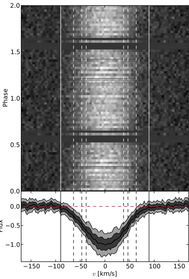
to extract the combined line profile we also need to subtract the continuum from the spectra. For that, we employed an iterative procedure masking out the line regions, based on the line list, and an estimated line width. For the LSD extraction of the line pro-file, we used the wavelength range 8000−9000 Å, resulting in a total of 50 available lines (with line depths greater than 0.5). The resulting line profiles have a velocity resolution of∼4 km s−1and signal-to-noise ratio of about 40−50. A radial-velocity-corrected trailed spectrum of all extracted profiles is shown in the top panel of Fig.8.
[image:6.595.41.291.281.447.2]A&A 532, A129 (2011)
[image:7.595.69.263.74.361.2]
Fig. 8.Radial velocity-corrected trailed spectrum (top) and the com-bined absorption line (bottom) resulting from the least square deconvo-lution for the data before the zenith break. Dark and light grey regions on the average line profile atthe bottom panelshow the 1-σand 2-σof the standard deviation throughout the orbit, respectively. Solid vertical lines depict the maximum allowed radius for the secondary star (i.e., its Roche-lobe radiusRL1). The vertical dashed lines mark the estimated radiusRMS(central lines) and the corresponding 1-σconfidence levels obtained from the RT by theχ2landscape technique.
between the radius corresponding to the secondary’s surface brightness calculated from the calibrated spectroscopic data and the radius implied by the photometric light curve. We therefore derive that parameter independently of the present data by per-forming a number of RT simulations with all parameters besides
RMS fixed, and determining the minimum of the resulting χ2. With this method, we obtain a radius of RMS = 0.16−+00..0603 R (=1.1+−00..42 ×1010 cm), which lies in-between the two possible radii of 0.8 and 1.6×1010cm fromPaper I.
We furthermore included gravity and limb-darkening cor-rections in the imaging procedure, using the coefficients from
Claret(2000). Finally, the instrumental broadening of the ab-sorption lines was accounted for by convolving the line profile with a Gaussian with full width at half maximum corresponding to the spectral resolution. FollowingWatson et al.(2007), we do not adopt a two-temperature model (Collier-Cameron & Unruh 1994). As with the Doppler tomography, only line profiles be-fore the occurrence of the flare were used. The resulting surface brightness distribution of LTT 560 is shown in Fig.9at five dif-ferent orientations. Brighter regions represent the “undisturbed” photosphere of the star and darker regions are spot-filled areas.
[image:7.595.332.527.91.331.2]The most prominent feature of the surface brightness dis-tribution is a large asymmetric spotted region covering most of the surface of the secondary star. This may be caused by one large spot covering a considerable fraction of the star, as e.g. ob-served byStrassmeier(1999) in the K0 giant HD 12545, or from a large group of smaller spots, with our data not allowing to
Fig. 9. The surface brightness distribution of the secondary star of LTT 560 as derived from the Roche tomography. The L1 face of the star is seen at phase 0.5. The circles mark a region around L1 (lower left plot: seen from the front side;lower right plot: seen through the star). Dark regions represent diminished absorption features of the line profiles, interpreted as spotted regions.
discern between the two scenarios. The observed asymmetry in the brightness profile is such that the back face of the secondary is less covered with star-spots (brighter) than the rest of the star, with a slight tilt in the direction of the stellar rotation. This is consistent with our result of Sect.3.3.1, i.e. that the leading side of the secondary appears to be the more active one.
4. Discussion
We have used Echelle spectroscopy of the PCEB LTT 560 to derive precise system parameters. From the metal abundances in the white dwarf photosphere, we determined an accretion rate of∼5 × 10⁻¹⁵ M
yr−1. Debes (2006) carried out a sim-ilar study of six white dwarf and main sequence binaries, both short-period (post-common envelope binaries, PCEBs) and wide binaries, and found accretion rates in the range 2 ×10⁻¹⁸ to 6 ×10⁻¹⁶ M yr−1. Their study includes the system RR Cae, a white dwarf plus M-dwarf binary that resembles LTT 560 in many aspects. Both systems have nearly identical white dwarf masses and similar companion star masses, but the orbital pe-riod of RR Cae is nearly double that of LTT 560.Debes(2006) determined an accretion rate of 4×10⁻¹⁶ M
yr−1 for RR Cae, and inferred, assuming a spherically symmetric wind and Bondi-Hoyle type accretion, a wind mass-loss rate of ˙MdM = 6 × 10⁻¹⁵ M
yr−1for the companion star. Taking the Bondi-Hoyle scenario at face value, ˙Macc∝1/R2, whereRis taken as the dis-tance between the white dwarf and the M dwarf. For an equally large wind mass-loss rate, the accretion rate in LTT 560 would be about three times higher than in RR Cae, which is only a fac-tor of about three below the accretion rate that we estimated from the photospheric abundances. Considering all the uncer-tainties involved in estimating the accretion rate and mass-loss
rate, RR Cae and LTT 560 appear to behave rather similar, and we speculate that it is the higher accretion rate in LTT 560 that is responsible for the chromosphere/corona around the white dwarf that we observe in Hα.
The accretion luminosity implied by M˙acc 5 × 10⁻¹⁵Myr−1isL1.8×1028erg s−1. Integrating the Hαflux, we find thatF(Hα)1.0×10⁻¹⁵erg cm−2s−1, or, adoptingd= 33 pc (Paper I),L(Hα)1.3×1026erg s−1, i.e. it is clear that the accretion-heated layer of the white dwarf must cool through additional emission mechanisms. InPaper I, we discussed how identifying LTT 560 with a nearby faint ROSAT PSPC source would imply an X-ray luminosity of∼6×1027erg s−1, which is comparable to the predicted accretion luminosity. A deep X-ray observation would be desirable to confirm the association of LTT 560 with the ROSAT X-ray source and to establish more accurately the flux and spectral shape of the X-ray emission.
The nearly identicalγvelocities of both the white dwarf’s Hαemission and the photospheric metal absorption lines suggest that they originate in the same region. However, because of the uncertainties involved we cannot exclude that the Hαemission is produced somewhat above the white dwarf’s photosphere. For a “worst case scenario”, we calculate the largest possible diff er-ence within the 3σuncertainties as
Δγ=γWD,metal+3σmetal−(γWD,Hα−3σHα)=2.15 km s−1.
Since the white dwarf radius is given byRWD =0.636MWD/vgr forM andRin solar units andvgrin km s−1,Δγtranslates into 0.11RWD. The Hαemission could thus in principle originate in a region up to∼1000 km above the photosphere. This still prac-tically excludes a “strong” shock as the mechanism behind the emission, because the associated shock height is inversely cor-related with the mass-transfer rate (e.g., Eq. (14) inFischer & Beuermann 2001), which for LTT 560 is two orders of magni-tude below that of even the low-accretion-rate polars (Schwope et al. 2002). It appears more likely that the emission line is pro-duced by heat deposited by the accretion resulting in a tem-perature reversal shortly above the white dwarf photosphere. However, a detailed treatment of the physics involved is beyond the scope of this paper.
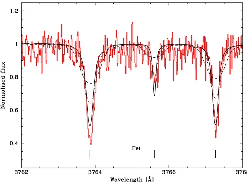
The narrow metal lines allow us to place a limit on the rota-tion rate of the white dwarf. Figure10shows a close-up of three Fe I lines, along with models forvsini =0, 15, and 30 km s−1, and suggests that the white dwarf in LTT 560 is a very slow (<∼15 km s−1) rotator, similar to the majority of single white dwarfs (Koester et al. 1998;Karl et al. 2005;Berger et al. 2005). This is an interesting result, as it suggests that the evolution of angular momentum of white dwarfs in PCEBs is similar to that of field white dwarfs, with current theories requiring magnetic torques to explain the observed low rotation rates (e.g.Suijs et al. 2008).
[image:8.595.307.554.74.256.2]The data sets used inPaper Iand the present one show the oc-currence of flares, indicating that there is an active secondary star in the system. Roche tomography shows an asymmetric surface brightness distribution, which we interpret as the presence of star spots (Fig.9). These high latitude and/or polar spots are very common in single active stars (e.g., Strassmeier et al. 2003), and have also been observed on donor stars of CVs (Watson et al. 2006,2007), as well as in the pre-CV V471 Tau (Hussain et al. 2006). The models ofGranzer et al. (2000) suggest that star-spots emerge preferentially from the flux tube close to the equa-tor of the star and are dragged by the Coriolis force to the pole of the star. Thus, high latitude and polar spots should be a com-mon feature on rapid rotators, such as close binaries. However,
Fig. 10. A close-up of three Fe I absorption lines in the white dwarf photosphere. Overplotted on the average spectrum are three TLUSTY/SYNSPEC models forTWD = 7500 K, logg = 7.75, and the abundances listed in Table3. The solid line shows a non-rotating white dwarf, the dotted line corresponds tovsini=15 km s−1, and the dashed line tovsini=30 km s−1.
we caution that these models are only valid for stars in the range 0.4M ≤M ≤1.7 Mthat contain a radiative core and a con-vective shell, and in LTT 560 the M5−6V secondary with a mass
MMS=0.14Mis well below this range and can be expected to be fully convective.
In addition to the high latitude features, we also observe that the inner face of the star in our model (the one facing the pri-mary) is slightly darker than its backside. The low latitude star-spots populating the region around L1 appear to be another com-mon feature in the tidally distorted late-type secondaries of close binaries (Watson et al. 2006,2007;Hussain et al. 2006). It has been suggested byHolzwarth & Schüssler(2003) that tidal in-teraction may force spots to appear at preferred locations.King & Cannizzo(1998) find the appearance of such spots at L1 to be the probable mechanism behind the low brightness states and mass-transfer variations in CVs. AsWatson et al.(2007) point out, a similar effect to that of star spots at L1 can be achieved by irradiation from the white dwarf primary, although the low tem-perature of the white dwarf (TWD =7500 K; Paper I) indicates that this effect will be small if important at all.
What kind of future awaits LTT 560? FollowingSchreiber & Gänsicke(2003)1, we calculate the period Psd at which the system becomes semi-detached as
Psd=2π ⎛
⎜⎜⎜⎜⎝ R3 MS
G MMS(1+q−1)(RL/a)3 ⎞ ⎟⎟⎟⎟⎠12
, (4)
taken fromRitter (1986), with the approximation of Eggleton
(1983)
RL/a=
0.49q23
0.6q23 +ln(1+q) 1 3
· (5)
With the parameters given in Table2(taking the average of the He- and the CO-configuration) and the secondary’s radius esti-mated from the RT, we find thatPsd = 1.52+−00..8543 h. The large
1 As already noted byZorotovic et al.(2010), Eq. (11) inSchreiber
& Gänsicke(2003) is incorrect in that the factor 9πhas to be replaced
A&A 532, A129 (2011)
uncertainty here is dominated by our insufficient knowledge ofRMS. Modelling the light curve of a photometric time-series data set of LTT 560 of high S/N would be desirable to improve the accuracy. Determining the distance to the system via a paral-lax measurement would similarly yield the absolute luminosities of the stellar components, thus provide independent access to bothRMSandRWDand the associated parameters. Nevertheless, aPsdbelow the period gap is consistent with the M5−6V spec-tral type of the secondary star (Beuermann et al. 1998;Smith & Dhillon 1998). Since it can be assumed that the secondary is fully convective, we use Eq. (8) fromSchreiber & Gänsicke
(2003) for angular momentum loss dominated by gravitational radiation to calculate the time it will take LTT 560 to start mass transfer via Roche-lobe overflow to∼3.5 Gyr. This is much less than the Hubble time, thus LTT 560 can be regarded as represen-tative of the progenitors of todays CVs. Since the system con-tains a non-magnetic white dwarf and the mass ratioq < 0.33, it is likely that the future CV LTT 560 will belong to the SU UMa subclass of dwarf novae.
Acknowledgements. We thank the anonymous referee for helpful comments. Many thanks also to Matthias Schreiber and Alberto Rebassa for enlightening discussions. This work has made intensive use of the SIMBAD database, op-erated at CDS, Strasbourg, France, and of NASA’s Astrophysics Data System Bibliographic Services. IRAF is distributed by the National Optical Astronomy Observatories.
References
Althaus, L. G., & Benvenuto, O. G. 1998, MNRAS, 296, 206
Asplund, M., Grevesse, N., Sauval, A. J., & Scott, P. 2009, ARA&A, 47, 481 Baraffe, I., Chabrier, G., Allard, F., & Hauschildt, P. H. 1998, A&A, 337, 403 Berger, L., Koester, D., Napiwotzki, R., Reid, I. N., & Zuckerman, B. 2005,
A&A, 444, 565
Beuermann, K., Baraffe, I., Kolb, U., & Weichhold, M. 1998, A&A, 339, 518 Claret, A. 2000, A&A, 363, 1081
Collier-Cameron, A., & Unruh, Y. C. 1994, MNRAS, 269, 814 Coluzzi, R. 1999, VizieR Online Data Catalog, 6071 Debes, J. H. 2006, ApJ, 652, 636
Dupuis, J., Fontaine, G., Pelletier, C., & Wesemael, F. 1993, ApJS, 84, 73 Eggleton, P. P. 1983, ApJ, 268, 368
Fischer, A., & Beuermann, K. 2001, A&A, 373, 211
Granzer, T., Schüssler, M., Caligari, P., & Strassmeier, K. G. 2000, A&A, 355, 1087
Holzwarth, V., & Schüssler, M. 2003, A&A, 405, 303 Hubeny, I., & Lanz, T. 1995, ApJ, 439, 875
Hussain, G. A. J., Allende Prieto, C., Saar, S. H., & Still, M. 2006, MNRAS, 367, 1699
Karl, C. A., Napiwotzki, R., Heber, U., et al. 2005, A&A, 434, 637
Kawka, A., Vennes, S., Dupuis, J., Chayer, P., & Lanz, T. 2008, ApJ, 675, 1518 King, A. R., & Cannizzo, J. K. 1998, ApJ, 499, 348
Kochukhov, O., Makaganiuk, V., & Piskunov, N. 2010, A&A, 524, A5 Koester, D., & Wilken, D. 2006, A&A, 453, 1051
Koester, D., Dreizler, S., Weidemann, V., & Allard, N. F. 1998, A&A, 338, 612 Kupka, F., Piskunov, N., Ryabchikova, T. A., Stempels, H. C., & Weiss, W. W.
1999, A&AS, 138, 119
Lanz, T., & Hubeny, I. 1995, ApJ, 439, 905 Marsh, T. R., & Horne, K. 1988, MNRAS, 235, 269
Panei, J. A., Althaus, L. G., & Benvenuto, O. G. 2000, A&A, 353, 970 Piskunov, N. E., Kupka, F., Ryabchikova, T. A., Weiss, W. W., & Jeffery, C. S.
1995, A&AS, 112, 525 Ritter, H. 1986, A&A, 169, 139
Ritter, H. 2008, Proceedings of the School of Astrophysics, Francesco Lucchin, Mem. Soc. Astron. Italiana, in press [arXiv:0809.1800]
Rutten, R. G. M., & Dhillon, V. S. 1994, A&A, 288, 773
Schmidt, G. D., Szkody, P., Vanlandingham, K. M., et al. 2005, ApJ, 630, 1037 Schmidt, G. D., Szkody, P., Henden, A., et al. 2007, ApJ, 654, 521
Schreiber, M. R., & Gänsicke, B. T. 2003, A&A, 406, 305
Schwope, A. D., Brunner, H., Hambaryan, V., & Schwarz, R. 2002, in The Physics of Cataclysmic Variables and Related Objects, ed. B. T. Gänsicke, K. Beuermann, & K. Reinsch, ASP Conf. Ser., 261, 102
Skilling, J., & Bryan, R. K. 1984, MNRAS, 211, 111 Smith, D. A., & Dhillon, V. S. 1998, MNRAS, 301, 767 Spruit, H. C. 1998, unpublished [arXiv:astro-ph/9806141] Strassmeier, K. G. 1999, A&A, 347, 225
Strassmeier, K. G., Pichler, T., Weber, M., & Granzer, T. 2003, A&A, 411, 595 Suijs, M. P. L., Langer, N., Poelarends, A., et al. 2008, A&A, 481, L87 Taam, R. E., & Ricker, P. M. 2010, New A Rev., 54, 65
Tappert, C., Gänsicke, B. T., Schmidtobreick, L., et al. 2007, A&A, 474, 205 Watson, C. A., & Dhillon, V. S. 2001, MNRAS, 326, 67
Watson, C. A., Dhillon, V. S., & Shahbaz, T. 2006, MNRAS, 368, 637 Watson, C. A., Steeghs, D., Shahbaz, T., & Dhillon, V. S. 2007, MNRAS, 382,
1105
Webbink, R. F. 2008, in Short-Period Binary Stars: Observations, Analyses, and Results, ed. E. F. Milone, D. A. Leahy, & D. W. Hobill (Heidelberg: Springer), Astrophys. Space Sci. Libr., 352, 233
Zorotovic, M., Schreiber, M. R., Gänsicke, B. T., & Nebot Gómez-Morán, A. 2010, A&A, 520, A86
Zuckerman, B., Koester, D., Reid, I. N., & Hünsch, M. 2003, ApJ, 596, 477