Model development for supporting advanced risk based approaches in air traffic management

(1)

April 29, 2014

MASTER THESIS

MODEL

DEVELOPMENT

FOR

SUPPORTING

RISK-BASED

APPROACHES

CENSORED

Nicole Havinga

Faculty of Electrical Engineering, Mathematics and Computer Science Stochastic Operations Research

Exam committee:

Prof. dr. Richard Boucherie (University of Twente) Dr. Judith Timmer (University of Twente)

Dr. Klaas Poortema (University of Twente) Ir. Roy Jansen (LVNL)

(2)

(3)

Summary

Occurrences are reported and investigated by Air Traffic Control the Netherlands (LVNL) as part of the safety management system. The purpose of this study is to develop a practical mathematical model which is able to analyse statistical characteristics of the available occurrence data. The intention is to use the results as part of more advanced risk-based approaches.

Model

The model developed uses the statistical characteristics of the data to support advanced risk-based approaches in safety assessment of LVNL. Supporting risk-based approaches is done by determining the practicability of reference values as suggested by FABEC, by identification of factors which con-tribute to risk, and by identifying relations between severity classes to give an indication of risk.

Risk-based approaches

Two reference values suggested by FABEC are studied on practicability, where each reference value is determined for major and serious incidents separately. The first reference value is practicable with exceedance probability 8.2·10−10 _{for major incidents, and with exceedance probability} ₃_.₀_·₁₀−1 _for

serious incidents. For the second reference value the exceedance probability is 9.7·10−1 _{for major}

incidents, and the exceedance probability is9.9·10−1_{for serious incidents.}

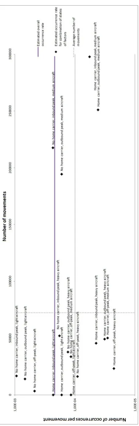
Two case studies are performed in identifying factors which contribute to risk. For the type of occur-rence ’deviation taxi’ the type of carrier, the type of peak and the type of aircraft are shown to contribute to risk. The states of the factors which contribute to risk are non-home carriers, inbound peaks, and light aircraft. The combination of states of factors which contribute to risk are: {non-home carriers dur-ing inbound peaks with light aircraft}, {non-home carriers during outbound peaks with light aircraft}, {non-home carriers during off-peaks with light aircraft},{home carriers during inbound peaks with light aircraft}, and{home carriers during inbound peaks with medium aircraft}. Where the first has an ex-traordinary contribution to risk.

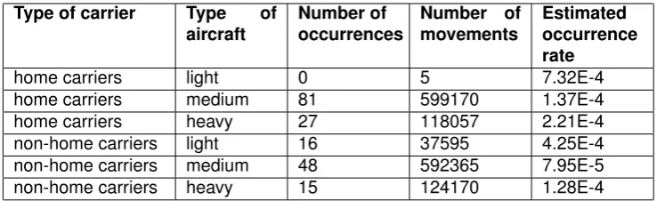
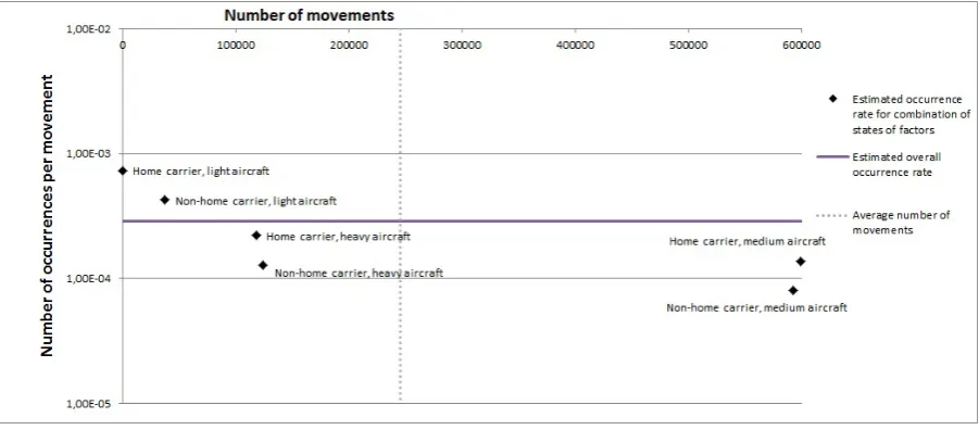
For the severity class major the type of carrier and the type of aircraft are shown to be factors which contribute to risk. The states of the factors which contribute to risk are home carriers and light aircraft. The combination of states of factors which contribute to risk are:{non-home carriers with light aircraft} and{home carriers with light aircraft}.

Relations between severity classes have been determined. The correlation between occurrences with no safety effect and occurrences with significant safety effect is strong, and thus the number of aircraft involved with occurrences of these severity classes have a dependency. The correlation between the other severity classes is weak or negligible, and thus independence is assumed. With this information on dependency, distribution functions are made for the ratio of severity classes. When severity classes are independent, the ratio is determined by using the Poisson distribution function. When severity classes are dependent on each other, the distribution is determined empirically by determining the mean and variance of the ratio.

Sensitivity analysis

Sensitivity analysis is performed on the results of the model by using confidence intervals and by adding data. The confidence intervals are considered to be sufficiently small. With adding data the numerical results change slightly, and thus conclusions on risk-assessment change slightly.

(4)

For risk-contributing factors: the same factors contribute to risk, and the combination of states which contribute (extraordinary) to risk remain the same for major incidents. For deviation taxi the same fac-tors contribute to risk, but the combination{home carriers, during outbound peaks, with light aircraft}is now determined to be risk-contributing, while{non-home carriers, during inbound peaks, with medium aircraft}is not anymore. Also, non of the combinations contribute to extraordinary risk anymore. When looking at the correlation between the number of occurrences in the severity classes, same con-clusions are drawn concerning the dependency of the severity classes.

Methods

The first method used to determine statistical characteristics of the data is the test of Kolmogorov-Smirnov to verify the presence of the Poisson distribution.

The second method used is Poisson regression, which identifies whether the influence of factors on the number of occurrences is observable. It also determines the degree of influence the factors have. Finally, Pearson’s correlation coefficient is used to determine the correlation between severity classes.

Recommendations

(5)

List of abbreviations

Abbreviations AAA Amsterdam Advanced ATC-system

ACAS Airborne Collision Avoidance System ACC Area Control Center

ANSP Air Navigation Service Provider

APP Approach

ATC Air Traffic Control CTA Control Area

FABEC Functional Airspace Block Europe Central IATA International Air Transport Association IFR Instrument Flight Rules

LVNL Air Traffic Control the Netherlands (Luchtverkeersleiding Nederland) NLR National Aerospace Laboratory

R/T Radio/ Telephony

RIASS Runway Incursion Alerting System Schiphol SID Standard Instrument Departure

SPSS Statistical program which is used for (part of) execution statistical methods

SSE Safety Significance Events; scheme which is used to classify severity of occurrences SSR Secondary Surveillance Radar

STAR Standard Arrival Routes

STCA Short Term Conflict Alert System TCAS Traffic Collision Avoidance System UDP Uniform Period Daylight

(8)

(9)

Chapter 1 Preface

This is the report for the graduation project at Air Traffic Control the Netherlands (LVNL) as part of the Masters-program Applied Mathematics at the University of Twente.

AppendicesCandDcontain confidential data/ output. The content of these appendices are left out in the public version of the report.

The research questions regarding the factors which play a role in the number of occurrences emerged whilst finishing my internship-project at LVNL this spring. It was clear that a model could be made to support LVNL’s risk-based approach. The research started out by focusing on the Kalman filter and its properties. Soon it became clear that another model was needed to achieve the set goals.

In the conversations with my first supervisor (Judith) about the structure of the data and the goals which were set, it became clear that the methods/ models studied in the courses of my study did not apply. Thus, we searched for models outside our courses and came to Poisson models.

Poisson models were not known widely by me, but when we first came across the term ’Poisson regres-sion’ it was clear that the method had potential for the goals which were to be achieved.

I looked deeper into the mechanism of Poisson regression and it indeed appeared to be very suitable. Also, as the Poisson distribution was required, we obviously looked deeper into the possibilities of this aspect.

Finding a distribution which was suitable for the number of occurrences for the different types led to the interest of studying the reference values. Being able not only to see whether the reference values were achieved in previous years, but also learning what the probability distribution looks like and determining the probability of exceeding the reference values.

Learning a distribution for the number of occurrences in the severity classes led to the thought of finding a (stochastic) ratio which indicates the relation between the severity classes when looking at the number of occurrences. Generally a fixed ratio is used. When the number of occurrences is stochastic, it seems logic that the ratio between these numbers is stochastic. Thus, the relation between the numbers is investigated on both dependency and value/ distribution.

Performing the study was a challenge in several ways. First because a steady mathematical model has to be built, whilst not loosing touch of the practical use. Second because the model requested did not exist yet, and the methods used were not yet known by me. There were many challenges on the way, but discovering new methods and combining them to a new model is what I liked best. A model is now at hand which used proper mathematical models, and is directly usable for LVNL in their risk assessment. It feels like an honor that I had the chance to create a model and than learn others at LVNL to use it.

I thank Judith for her support as first supervisor. Even when we did not agree on whether a method was suitable or not, the discussions were good and even pleasant. You have been supportive all the way through. You listen patiently and have a positive way of giving advise and feedback. When I was looking at new methods you always put effort in looking into them as well. That made the discussions well-funded and effective, and also enjoyable.

(10)

Also, I would like to thank Richard for starting as second reader and becoming first reader at the end of this project. The clear instructions on how to finish the project helped in completing it without too much delay.

I would also like to thank Klaas for the support he gave during both my internship and my graduation project with my questions regarding statistics. I appreciate your patience in answering questions about both SPSS and the theory in statistics.

(11)

Chapter 2 Background, introduction problem,

goals

2.1 Background

Air Traffic Control the Netherlands (LVNL) is responsible for providing air traffic services within the flight information region Amsterdam, and provides communication-, navigation- and positioning-services. Other responsibilities lie in the provision of aeronautical information services and publishing aeronau-tical publications and maps. Also providing training for air traffic safety is an important responsibility, as well as advising both the Minister of Infrastructure and Environment, and the Minister of Defense on matters in the field of civil air traffic management. The responsibility also lies in carrying out other duties assigned by the aviation law [1]. A part of this responsibility thus lies in directing all aircraft at and around the mainport Schiphol.

Mainport Schiphol handles on average 1400 flights a day. For all arriving, departing and transiting air-craft is a schedule, these possible activities are called movements. Deviating events which take place are reported and analyzed, these events are calledoccurrences. An event is an occurrence if it fulfills one or more of the following descriptions [2]:

1. Loss of separation between an aircraft and one or more other aircraft and/ or ground-vehicles. 2. An aircraft or ground-vehicle which deviates from an ATC instruction or procedure.

3. An aircraft or ground-vehicle which follows wrong instructions given by an ATC or to which no instruction is given.

4. Inability or decreased ability to supply ATC services and/ or failure of technical functions.

Every occurrence which lies in the responsibility of LVNL is reported and undergoes an analysis, in which five steps are taken to classify the severity of the occurrence. The occurrences are added to the database, which is used to perform research; e.g., based on the data, research is performed to check whether there is a need to adjust the ATC system (e.g., procedures, equipment, training, etc.).

2.2 Introduction to problem

The current occurrence database is filled with occurrence data starting on January 1st 2010 and is a rich source of information. LVNL wants to learn as much as possible from this database, the question is how to learn from it without losing grip on the complete picture.

The occurrences taken into account in this study are those which took place at ACC, APP and at Schiphol airport. The reason for this is that the responsibility for these airports lie (completely) at LVNL, at other airports in the Netherlands more parties have influence (for example hobby-flights which arrive and depart). Moreover, the influence factors considered in this study are aimed at the infrastructure and procedures of mainport Schiphol.

(12)

This study focuses on factors which are specified per flight; e.g. type of carrier, type of peak in which the flight took place, and type of aircraft used. This new focus requires a new model, where the aim has been set on Poisson models. The benefits of Poisson models is that they are developed to analyze the statistics concerning events which do not happen with a high average.

The goal of this study is to support risk-based approaches. This includes investigating the practicability of reference values, identifying factors which contribute to risk, searching for relations between types of occurrences and their severity, and finding relations between the number of occurrences in the severity classes.

Research questions stated by LVNL are stated in section2.3.

2.3 Goals

The main goal of this study is:

Model development and analysis for occurrence data in air traffic management to support advanced risk-based approaches

The following research questions are posed:

- How can LVNL’s risk-based approach be supported by the available data?

1. How can statistical characteristics be used to test reference values on practicability? 2. How can circumstances which contribute to risk be identified?

- Which circumstances influence the number of occurrences of a certain type. - Which circumstances influence the number of occurrences of a certain severity. 3. How do the number of occurrences in the severity classes relate to each other? - Which statistical characteristics can be found concerning the occurrence data?

1. The distribution for the number of occurrences which take place per month; for all types of occurrences and for all severity classes.

2. The relation between the type of occurrences and their severity classifications.

3. The relation between the type/ severity of occurrences and the circumstances concerning occurrences.

(13)

Chapter 3 Literature review

This study analyzes occurrence data in air traffic management where support of a risk-based approach is one of the major issues. The literature investigated can be divided in three categories, namely: relevant research in adjacent fields, methods for investigating statistical characteristic of the data, and difficulties in (supporting) risk-based approaches.

Adjacent fields

There are several adjacent fields to look for occurrence data analysis, some fields which are considered are in road traffic accidents, ship accidents, and other studies for air traffic accidents.

In 2009 LVNL and the NLR published a paper [3] which presents safety criteria concerning ATC-related risk, this article relates to this study in the sense that it searches for accident probabilities, which is of interest to this study since statistical characteristics of the data are sought. The article finds a way to express the ”accident probability related to separation between aircraft and other aircraft, their wake vortices and vehicles”. However, the model of the study is not used in this study since the search is for a model which shows statistic characteristics and influences for occurrences in more detail. Note: an occurrence is not always an accident.

The same year the NLR published the report called the ”Causal model for Air Transport Safety”, where a causal model is built to get a ”thorough understanding of the causal factors underlying the risks of air transport and their relation to the different possible consequences so that efforts to improve safety can be made as effective as possible”[4].This study is of interest since it looks at factors which have a possible influence on the number of occurrences, as is required in this study. However, a model is sought for finding statistical characteristics of the data, the model proposed is a causal model and thus lies outside the scope of this study.

Time-series analysis of road risk is performed in [5] where it discusses several time-series analysis models. These types of models are of interest due to the fact that they provide insight on the devel-opment of accidents through time and the underlying reasons of how they originate. However, these models are used ”as a tool to describe, explain and predict changes in the trends of the road safety level”, where this study focuses on the statistical characteristics of the data rather then on the predic-tions for the future. Some of the (time-series) methods have been studied to apply nontheless, but eventually turned out to be inappropriate for the goals of this study.

(14)

Methods for investigating statistical characteristics

Several statistical characteristics are of interest, the subjects of interest are: • (Tests for) the distribution of the number of occurrences.

• Factors which influence the number of occurrences (of certain types). • Relation between the type and the severity of occurrences.

In [11] the normal distribution has been investigated for the number of occurrences in the separate severity classes and seasons. This distribution was not applicable for every case, and thus the search for fitting distributions is ongoing. Beside the interest for the distributions for the number of occurrences in the severity classes, there is a growing interest for the distribution on the number of occurrences for the different types of occurrences. Since occurrences can be divided over dozens of types, the distribu-tion which is searched for should be able to handle countable events which do not appear very often. A distribution that comes to mind is the Poisson distribution, as it is a distribution which counts the number of occurrences (with low averages) in a certain time-frame.

Determining whether the occurrences take place according to a Poisson distribution can be done by the statistical test called the Kolmogorov-Smirnov test [10]; this test compares the empirically found distribution to the assumed distribution.

Once distributions are found, regression analysis can be used when looking at factors which influence the number of occurrences. This has also been done in [11]. The focus is on factors which influence occurrences of specific types or severity, a different type of regression than in [11] is necessary to get the desired results. Poisson regression is in place when looking for influence factors for the type and severity of occurrences when the average number of occurrences is low. In contrast to many other types of regression, Poisson regression can handle integer valued output variables without problems (in this case the number of occurrences). In Poisson regression the Poisson distribution is assumed for the number of events, which is verified with the Kolmogorov-Smirnov test.1

Once distributions and influence factors are found, the focus shifts to the severity classes. Each oc-currence is of a certain type (sometimes multiple types) and a severity class. Knowing the distributions and the influence factors leads to investigation of the division of occurrences over the severity classes. Poisson processes and their characteristics (as described in [12]) are investigated to determine which type of occurrences leads to the different severity classes and with which rate. This way not only the distribution of the severity classes are found, but also the way in which they are built up from the different type of occurrences. The difficulty lies in the requirement of the Poisson processes to be independent for each other to use the desired properties, which is not the case in the organization of the database as shaped by LVNL; an occurrence can be several types at once, where certain combinations are strongly correlated.

Difficulties in (supporting) risk-based approaches

One of the goals of this study is to support an advanced risk-based approach. A swift look has been given to risk analysis in other fields, but this did not give an appropriate method. Many risk-based approaches are aimed at the (possible) damage incurred by occurrences; this can be expressed as either money, lives, etc.. This is not applicable for the situation of this study, since in most cases there is no measurable amount of damage; this is done in [13], also [14] discusses multiple models. This makes it hard to quantify risk, and is thus the reason why statistical characteristics on occurrence data is studied and not the quantification of risk.

(15)

Chapter 4 Available data and its structure

This section gives a description of the structure of the data which is used as input for this study, starting by the types of occurrences and the dependencies therein. Followed by a description of the severity classification which takes place for each occurrence.

4.1 Types of occurrences

A part of the occurrence database is the classification of the ’types’ of occurrences. The types focus on the description of the sort of occurrence; also known as ’what-classification’. It is important to realize that one occurrence may exist of multiple types (often two or three), as more than one description is needed to describe the entire occurrence. Due to this characteristic of the occurrences (and thus of the data), the conclusion is drawn that there is a dependency between the possible types, this is discussed and shown in appendixC.2.

Also, some new types of occurrences have been added and some old types of occurrences have been split up through time. This requires some fitting of the data to obtain meaningful results and is discussed below.

Dependencies in types of occurrences

Many mathematical models require independence of variables. Models immediately lose their usabil-ity when this fundamental requirement is not fulfilled. In this study a relationship between the type of occurrence and the severity class of an occurrences is sought, the problem with this is that the types of occurrences are sometimes closely related. Many models are viewed to quantify the relation but all assume independence of the variables (and thus independence of the different types of occurrences). The dependency of the different types of occurrences lies in a few things. First of all, an occurrence (especially a severe one) is often an assembly of events and thus multiple things can be appointed to the occurrence in regard to the things which did not follow procedure. For example: aircraft a acci-dentally ’enters the runway without clearance’, which causes a ’missed approach’ for landing aircraftb

which thus makes a ’go around’ to try landing again later. During this go around an ’airborne-separation’ occurs between aircraftband another approaching aircraftc. This is all denoted as one occurrence, this example shows that an occurrence can be a gathering of events.

Also, some types of occurrences are strongly related since one often cannot appear as an occurrence without the other. For example: a serious incident in the air always includes multiple aircraft which are too close to each other (’airborne separation’), in principle a cause for the lack of separation can be indicated; which is thus filed as another type.

Another dependency lies in the connection with the severity classes, when an ’airspace infringement’ is involved in a serious incident, then there has also been an ’airborne separation’.

(16)

When analysis is desired for the relationship between the types of occurrences and the severity classes it is important that the variables taken into account are independent of each other. One way to accomplish this is by dividing the types into groups which are independent of each other. To illustrate how the type of occurrences can be grouped, three suggestions are given in appendixC.2.

The first suggestion is selecting occurrences on the location of the occurrence, in other words: in which part of the organization the occurrence took place. The parts of the operation are subdivided in ACC, APP, ground-control, or on the runway.

The second suggestion is subdividing the types over cause and effect: is the type of occurrence a cause of the occurrence, or is it the effect of something else.

The third suggestion is subdividing types over flight-phase. A flight at Schiphol airport has several phases, a departing flight has the phases start-up and push-back, line-up, taxiing, take-off, departure, and CTA outbound. An arriving flight has the flight phases CTA inbound, initial and intermediate ap-proach, final apap-proach, landing, and taxiing. A transit flight only has flight-phase CTA transit.

The difficulty in grouping the types is that it is not a one-on-one transformation, some types belong in multiple classes of the groups. Moreover, expert judgment is used to subdivide the different types over the classes, which is thus not defined exactly but somewhat based on a personal view. Where most types have one clear class, some are in a gray area between the classes and thus belong in multiple classes.

A definite conclusion cannot be drawn on how to group the different types of occurrences in such a way that all classes of occurrences are independent of each other. Further research is needed to find a way to cope with the dependencies.

Fitting data - combining types of occurrences

A number of what-categories has been added or changed during the period in which data was gath-ered, some are new categories and others are old categories which have been split. Categories which have been split are combined to their original category, new categories are gathered in the old category ’other’ since these used to be registered there. Also a few categories with very few occurrences and a clear overall category are combined to the overall category (such as Emergency - Mayday, Emer-gency - Medical, EmerEmer-gency - Panpan, EmerEmer-gency - VOS, EmerEmer-gency / Other; these are combined to Emergency). All combined categories are stated in appendixC.1.

4.2 Severity classification

Occurrences are reported at LVNL, which can be nearly anything: an aircraft which enters the taxiway without clearance, but also an emergency landing. Every reported occurrence undergoes an analysis performed by the department Performance in co-operation with specialized air traffic controllers. The analysis exists of five steps [15]:

1. Gather information 2. Analyze information

3. Categorize according to ’Safety Significant Events’-scheme (SSE) 4. Formulate conclusions

5. Formulate recommendations

Step 2 and 3 of the occurrence analysis are of particular interest in the data analysis. The second step indicates to which type the occurrence belongs; e.g. an aircraft has deviated from the planned route, an emergency call has been made, etc. The third step classifies occurrences on severity based on guidelines, these guidelines take into account the number of aircraft/ vehicles involved, whether or not a loss of separation has occurred, and who detected and/ or solved the problem.

(17)

The combination of the above and the one who detects/ solves the occurrence determines the sever-ity.

The severity classes are designed as follows (in increasing order of severity) [15]: - No safety effect

• Unilateral occurrence, or

• Effective ATC solution and no loss of separation - Significant incident

• Effective ATC solution and a significant loss of separation, or • ATC safety barriers worked and a limited loss of separation, or

• Less effective ATC solution or airmen solved the event and no loss of separation - Major

• ATC safety barrier worked and a major loss of separation, or • Less effective ATC solution and a significant loss of separation, or • ATC safety barrier did not work and a limited loss of separation, or • No ATC safety barriers worked and no loss of separation

- Serious

• ATC safety barriers did not work and a significant loss of separation The following definitions are used [15]:

- Major loss of separation:≤50%of needed separation - Significant loss of separation:≤66%of needed separation - Limited loss of separation:>66%of needed separation

(18)

(19)

Chapter 5 Assumptions

This study has some assumptions regarding the data and the used models. This section discusses the assumptions and illustrates why they are plausible.

The first assumption is that the data used for this research can be considered as reliable. The per-formance department plays a central role in securing the reliability. Also, all experts are trained and a handbook is available with clear definitions on how to report and analyze occurrences. Also the system supports a consistent working method.

The second assumption regarding the data is that it is uniformly defined: the working methods of LVNL has not changed drastically since the start of the occurrence database on January first 2010. Some small changes have been made in secondary definitions during the four years of filling the database: some types have been split up in multiple types to gain an even more precise insight. These changes can be corrected by changing the new types back to the old types, this is described in section4.1. The third assumption is that all occurrences registered are taken into account. This consists of all oc-currences reported by LVNL personnel, and reports of others to LVNL such as airlines and Schiphol airport. LVNL has the policy of registering all occurrences, no matter how insignificant it may seem. However, a guarantee cannot be given that some occurrences slip through the system. Also, all occur-rences studied are related to the operations of LVNL and are ATC-related

The fourth assumption is that occurrences are independent of each other. When multiple aircraft are part of an occurrence, they are registered as the same occurrence.

Though the occurrences are assumed to be independent of each other, the different types of occur-rences are not. This aspect is studied in section 4.1and arises from the fact that multiple things can deviate from procedures during one occurrence.

Furthermore, LVNL started the database in its current form in January 2010, thus the data can be used from that moment on. The primary data used in this study therefore stems from 01-01-2010 till 31-12-2012, which is exactly three years of data. The data from 01-01-2013 till 31-12-2013 is used for sensitivity analysis on the output of the model.

Finally, the occurrences taken into account are those which occurred at and around Schiphol airport, which includes: Schiphol airport and the airspace which is under control of LVNL.

The occurrences at Rotterdam airport are not taken into account, since it differs from Schiphol airport. Adding occurrences on Rotterdam airport would influence the output of the models incorrectly. E.g., Rotterdam airport has no peak-times due to the fact that there is one runway, also home-carriers are defined as those airlines which have Schiphol airport as home base. The model can be used for occur-rences at Rotterdam airport, but a separate analysis is needed.

(20)

Summarized:

1. The dataset is reliable.

2. The dataset is uniformly defined; new types of occurrences can be changed back to the original types.

3. All occurrences registered by LVNL are taken into account. 4. Occurrences are independent of each other.

5. Initial data used stems from 01-01-2010 till 31-12-2012, data from 2013 is used for the sensitivity analysis.

(21)

Chapter 6 Model

The model is developed to support LVNL in it’s risk-based approaches. It is thus made to perform risk-assessment in several ways. The first section (6.1) describes why and how three subjects of risk-assessment are supported.

The subjects in risk-assessment are: finding circumstances which contribute to risk, verifying the prac-ticability of reference values, and finding a relation between the number of occurrences in the different severity classes.

Occurrences and their properties for supporting these subjects in risk-assessment can be described by three elements: the factors describing the circumstances of occurrences, the types of the occurrences, and the severity of the occurrences. Properties of these elements are described (mathematically) in section6.2.

The relations between the elements describing occurrences are stated in section6.3. These relations are used to support risk-assessment.

The analysis of the model for risk-assessment is described in section7.

6.1 Description of the model

The first part of the model for risk-assessment is developed to determine the relation between occur-rences and their circumstances. The circumstances are described by factors, where the states of the factors indicate the specific circumstance of that type which is present; e.g., the factor ’type of carrier’ has the states ’home carriers’ and ’non-home carriers’. These factors are not only determined for the occurrences, but also for each movement which takes place.

The (degree of) influence of the factors is determined with Poisson regression. Poisson regression first establishes if there is a significant influence for each factor, next it determines the degree of influence; Poisson regression and its use is described in appendixA.3. The influence which circumstances have on the number of occurrences is used to find circumstances which contribute to risk. Circumstances in which more than average occurrences take place are viewed as risk-contributing; this analysis is described in more detail in section7.2.

The second part of the model in risk-assessment concerns practicability of reference values. Gov-ernments are developing legislation on the number of occurrences which is acceptable, thus reference values are being developed. This legislation is intended to safeguard air-traffic safety. Thus, there is a need to determine whether these reference values are practicable, which can be done by using a statistical model. The probability that these reference values are (not) exceeded can be determined by using the statistical distribution for the number of occurrences; this detailed analysis for this is described in section7.1.

Thus, a distribution is sought for the number of occurrences which take place. The Poisson distribution is used as it is known to work well when events occur with a low average. The number of occurrences is counted for each severity and for each type of occurrence, the average number of occurrences is low for the types and severity classes. The presence of the Poisson distribution is verified by using the statistical test of Kolmogorov-Smirnov; which is described in appendixA.2.

(22)

An effort is made to find a relation between the type of occurrence and its severity. This relation can identify risk and thus where an adjustment in the operational procedure of LVNL should be focused on. When for example a specific type of occurrence leads mostly to a high severity, then one could consider extra effort in preventing this type of occurrence. Details and difficulties of this relation is discussed in section6.3.

6.2 Main elements of the model

To support risk-based approaches it is necessary to first describe occurrences and their properties. The properties of occurrences are defined in three (main) elements in the model. These elements are described in this section: factors describing the circumstances of movements/ occurrences, types of occurrences, and severity of occurrences.

Factors

Factors(f) describe the circumstances of the movements, these factors have a potential influence on the number of occurrences which take place. The influence can be on a specific type, as well as a specific severity of occurrences. A specific factorfk consists of several statesc, these states describe the alternative options of the factor. The factors are thus categorical. Factorkin statecis denoted by

fck, thus:

Definition 6.2.1 (Factors). Factors describe the circumstances of movements and have a potential influence on the number of occurrences.

Definition 6.2.2(States of factors). Factorkexists of the union of statesc, where factorkin statecis denoted byfk

c:

fk = [

c

fck

Examples of factors are the ’type of carrier’, ’type of peak’, and ’type of aircraft’. The states of these factors are respectively{home carriers, non-home carriers},{inbound peak, outbound peak, off-peak}, and{light aircraft, medium aircraft, heavy aircraft}.

When looking at movements and occurrences, several factors are needed to describe all circumstances. The entire set of factors to describe the circumstances of movements is given byFT_{, which is the union}

of all available factorsfk_{. So:}

Definition 6.2.3(Set of factors). The set of factors describing the circumstances of movements is given byFT _{and is the union of all factors}_fk_:

FT = [

k

fk

When making an analysis not all factors are taken into account, only those which are of interest. The set of factors taken into account is denoted byF, which is a subset ofFT_:

Definition 6.2.4(Set of factors for analysis). The set of factors used when making an analysis is given byFand is a subset of all factorsFT:

F ⊂ FT

When a set of selected factors is taken into account and the states of the factorsfk _are_c_{, then the}

combination of states of the factors is denoted byFC:

Definition 6.2.5(Combination of states of factors). The combination of factorsfk _{in specific states}_c_is

given byFC(the combination of the states is given byC), which is the union offck:

FC =

[

k

(23)

Types of occurrences

As stated in section 2.1: an occurrence is defined as a deviating event. The type of an occurrence indicates which deviation took place. Since multiple deviations can take place at the same time, multiple types can be allocated to one occurrence. The set of types is given byI, and typeiis an element ofI

(i∈I).

Multiple aircraft can be involved in an occurrence (often two), and thus the number of aircraft involved with occurrences is counted rather than the number of occurrences. Counting the number of aircraft involved with occurrences can either be doneper movement (denoted byT_i∗), orper month(denoted byTi). Where the first is called theoccurrence rate for type i occurrences, and the latter has a Poisson

distribution with rateλi.

Definition 6.2.6(Occurrence rate for type i occurrences). The number of aircraft involved with occur-rences per movement for occuroccur-rences of type iis given byT_i∗ and is called the occurrence rate for type i occurrences.

Assumption 6.2.7 (Distribution for type i occurrences). The number of aircraft involved with occur-rences per month of typeiis given byTiand has a Poisson distribution with parameterλi:

Ti ∼ P oisson(λi)

When used, assumption 6.2.7is verified with the Kolmogorov-Smirnov test; which is described in appendixA.2.

Severity of occurrences

The severity of an occurrence is allocated according to the scheme given in section 4.2, the set of severity classes is given by J = {no safety effect, significant safety effect, major incident, serious

incident}; in contrast with the type of occurrences, only one severity can be allocated to an occurrence. The number of aircraft involved with occurrences per movement of severityjis given byS_j∗; also called theoccurrence rate for occurrences of severity j.

Definition 6.2.8(Occurrence rate for occurrences of severity j). The number of aircraft involved with occurrences per movement for occurrences of severityj is given byS_j∗ and is called the occurrence rate for occurrences of severity j.

The number of aircraft involved with occurrences is also determined per month for each severity class, given bySj. The number of occurrences per month have a Poisson distribution for each severity

class with Poisson parameterλj.

Assumption 6.2.9 (Distribution for occurrences of severity j). The number of aircraft involved with occurrences per month of severityjis given bySjand has a Poisson distribution with parameterλj:

Sj ∼ P oisson(λj)

As before, assumption6.2.9is verified with the Kolmogorov-Smirnov test whenever it is used.

6.3 Relations between and in the main elements of the model

To support risk-based approaches it is necessary to determine the relation between the elements of the model. Several relations are established: relations between the factors and the type/ severity of occurrences, relations between the type and the severity of occurrences, and relations between the number of occurrences in severity classes. Each of the relations is described below.

Relation between factors and types / severity of occurrences

A relation is found between factors as described in section 6.2 and the number of (aircraft involved with) occurrences. A relation can be given with respect to the type and with respect to the severity of occurrences.

For the types of occurrences the relation is described as the occurrence rate of type i for the com-bination of states of factorsFC. This relation is denoted byTi∗(FC), wherei∈I.

Similarly: for the severity of occurrences the relation is described as the occurrence rate of severityj

for the combination of states of factorsFC. This relation is denoted bySj∗(FC), wherej∈J.

Definition 6.3.1 (Relation between factors and the types of occurrences). The relation between the number of aircraft involved with occurrences per movement of typeiand a set of factors in given states

(24)

Definition 6.3.2(Relation between factors and the severity of occurrences). The relation between the number of aircraft involved with occurrences per movement of severityj and a set of factors in given statesFCis given bySj∗(FC).

The relation between the factors and the occurrence rates for the different types and severities is used for risk identification. For example: an occurrence rate which is significantly higher than average for certain circumstances can be used as an identification for circumstances which contribute to risk. Statements on determination of contributing factors, contributing states of factors, and risk-contributing combinations of states of factors are described in detail in section7.2.

Relation between types and the severity of occurrences

A relationship exists between the number of aircraft involved with occurrences per month for the types and severity. When the relation between a certain type of occurrence and a severity class is strong one could draw conclusions on the contribution to risk of the type.

For example: when a certain type leads mostly to severe incidents, a strong contribution to risk could be assumed and thus preventing this type of occurrences could get higher priority. The other way round: when a certain type never leads to a high severity, it probably does not need highest priority on prevent-ing it.

The relationship between types of occurrences and their severity is given by Sj = g(Ti). This

rela-tionship is not one-to-one for several reasons. First because each type of occurrence can lead to each severity. The second reason is because an occurrence can be of several types at once, but only of one severity. The difficulty of this is explained below.

Definition 6.3.3(Relation between types and the severity of occurrences). The (not one-to-one) relation between types and the severity of occurrences is given bySj=g(Ti).

Having an occurrence which is of several types counts as one occurrence for each of these types. Since it is one occurrence, only one occurrence is counted for the corresponding severity class. Simply adding the occurrences from the separate types of occurrences to a corresponding severity class then leads to a higher count of occurrences than actually took place; e.g., an occurrence of types ’airborne separation’ and ’airspace infringement’ of severity ’major’ counts as one for each type and one for the severity class ’major’. Thus, a correction factor is necessary to get the accurate number of occurrences for the severity class.

In determining the relation, one can use the Poisson distribution which is known for the number of aircraft involved with occurrences for each type of occurrence. For each type of occurrence a distribu-tion can be found (empirically) on which part of the occurrences of typeileads to which severity class. Recall, a correction factor has to be included in the relation.

A few aspects should be taken into account when determining the correction factor. The most important are: the frequency in which combinations of types take place in one occurrence, and the (average) number of types allocated to an occurrence of a certain severity.

The first aspect is based on the fact that certain combinations of types take place in the same occur-rence often, whereas some combinations never take place in the same occuroccur-rence. For example: the types ’airspace infringement’ and ’airborne separation’ often take place at the same time, whereas ’de-viation taxi’ and ’airborne separation’ never take place in the same occurrence; the latter cannot occur simultaneously as the first is on the ground and the second is a loss of separation between multiple aircraft which are airborne. An indication of the combination of types which take place simultaneously is given in appendixC.2.

The second aspect is based on the knowledge that severe occurrences often have more types attached than occurrences with no safety effect. Thus, the correction factor should not only be based on the types of occurrences, but also on the types of occurrences combined with the severity of the occurrences. When a correction factor is determined and a direct expression is found for the relation between the type and severity of occurrences, one can compare the determined value ofSj with the corresponding

pre-determined Poisson distribution and its parameter (λj).

A suitable correction has not been found due to the complexity of the relation.

Relation between the number of aircraft involved with occurrences in severity classes

(25)

So: assume severity classiis of lower severity than severity classj, with resp.SiandSj occurrences.

The fixed factor between the number of occurrences of the severity classes isR, thusSi=R·Sj.

The factor can thus be seen as the ratio between the number of (aircraft involved with) occurrences in two severity classes, denoted byR= Si

Sj wherei6=j.

The number of (aircraft involved with) occurrences in the severity classes has a Poisson distribu-tion. This can be used to find a distribution for the ratio R when the number of occurrences in the severity classes are independent of each other. The distribution can be determined empirically when independence cannot be assumed. The distribution functions for the ratio’s are given in section7.3. Definition 6.3.4(Relation between the number of aircraft involved with occurrences in severity classes). The ratio for number of aircraft involved with occurrences in severity classiand severity classj(i6=j) is given byR= Si

(26)

(27)

Chapter 7 Analysis

This section describes how the model is analyzed to support the three subjects in risk-assessment as mentioned in section6.

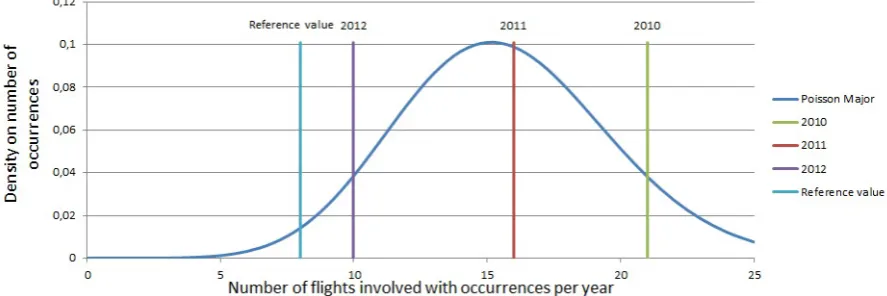
It first shows how the Poisson distributions are used to determine the probability of (not) exceeding the given reference values in section7.1. Recall: reference values are developed by governments to safeguard air-traffic safety, the analysed reference values are indicative.

Next, section7.2describes how the results of Poisson regression are used to identify if and how factors/ circumstances contribute to risk. Statements are made on how risk is defined.

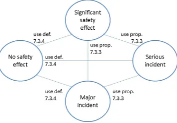
Last, section7.3describes how the relation between the number of occurrences in the severity classes is used in risk-assessment. It describes how a distribution function can be found for the ratio as dis-cussed in section6.3.

7.1 Practicability of reference values

Testing the practicability of reference values starts by determining the Poisson distribution for all severity classes of occurrences, this is done with the test of Kolmogorov-Smirnov. The Poisson distribution is determined for the number of flights involved with occurrences per month for each severity class:

Sj ∼ P oisson(λj)

Where:

Sj := Number aircraft involved with occurrences of severityjper month,j ∈J

WhereJdenotes the set of severity classes.

Reference values are given by F ABEC and are defined with different units for measuring traffic volume, the unit is thus translated to the number of aircraft involved with occurrences per year:

r := Given reference value, unit as traffic volumev,r∈R, whereRdenotes the set of reference values.

ˆ

r := Reference valuertransformed to unit ’number of aircraft involved with occurrences per year’. The Poisson distribution is determined for the number of aircraft involved with occurrences per month. It is transformed to the Poisson distribution with a parameter for the number of aircraft involved with occurrences per year. This is done by summing the Poisson parameter of twelve months, which can be done since the months are assumed to be independent and all have Poisson distribution with equal mean. So:

ˆ

Sj ∼ P oisson(12·λj)

ˆ

Sj := Number aircraft involved with occurrences of severityjper year

Next the practicability of the reference value is verified by observing the exceedance probability, which is done by:

P( ˆSj>rˆ) = 1−P( ˆSj ≤rˆ)

= 1−

brˆc

X

k=0

(12λj)k

k! ·e

−12λj

(28)

and givenα:

α = P(X >ˆr) = 1−

brˆc

X

k=0

(12ˆλj)k

k! ·e

−12ˆλj

And thus:

1−α =

brˆc

X

k=0

(12ˆλj)k

k! ·e

−12ˆλj

Note:αis given andλˆjis to be determined

Statements for the determination of the practicability of a given reference value are:

Proposition 7.1.1(Practicability of reference values (1)). A reference valueris practicable with proba-bility1−αif the exceedance probability is equal toα.

Proposition 7.1.2(Practicability of reference values (2)). A reference valuerˆis practicable with (given) probability1−αif the number of flights involved with occurrences is on averageXˆ

P( ˆX >rˆ) = α

7.2 Determination of risk-contributing factors

The model determines whether factors and their states contribute to risk by studying the occurrence rate for the different circumstances. A situation which contributes to risk is seen as those (combinations of) circumstances which lead to more than average occurrences of a certain type or severity. Thus, the occurrence rates are determined for each combination of (states of) factors and are compared with each other.

It is first determined whether factors contribute to risk. Next it is determined which states of the factors contribute most to risk, in other words: which state of the factor has the highest occurrence rate when the states of the other factors are kept equal. Following, the occurrence rates for the com-binations of states of factors are determined to identify whether comcom-binations lead to a higher than average occurrence rate, and thus which combinations contribute to risk. Last, it is determined which combinations of states of factors lead to an extraordinary contribution of risk, which is seen as combi-nations with an occurrence rate which is above average and which have more than average movements. Starting by the contribution of risk of factors: a factorfkis said to contribute to risk when the occur-rence rate for the statescof the factor differ significant.

Poisson regression determines whether the factors have a significant influence on the number of oc-currences. When it determines a significant influence it indicates that the states of the factors lead to a significant difference in the number of occurrences. So: when Poisson regression determines a significant influence for a factor, it is directly stated that the factor contributes to risk.

Definition 7.2.1(Risk-contributing factors). A factorfk_{contributes to risk if the occurrence rate for the}

statescof the factor differ significant.

Factorfk_{contributes to risk for occurrences of type}_i_when:

T_i∗(f_ck) 6= T_i∗(f_ck∗)∃c6=c∗

Factorfkcontributes to risk for occurrences of severityjwhen:

Sj∗(fck) 6= Sj∗(fck∗)∃c6=c∗

WhereT_i∗(fck)denotes the occurrence rate for occurrences of typeiwith statecof factorfk, andSj∗(f k c)

denotes the occurrence rate for occurrences of severityj with statecof factorfk.

(29)

Definition 7.2.2(Strongest risk-contributing state of a factor). A state ¯c of risk-contributing factor fk

contributes strongest to risk for occurrences when factorfk contributes to risk, and state¯cleads to a higher occurrence rate than other statescof factorfk_.

State¯cof risk-contributing factorfk _{contributes strongest to risk for occurrences of type}_i_when:

T_i∗(f_ck) 6= T_i∗(f_ck∗)∃c6=c∗ and

T_i∗(f_¯_ck) > T_i∗(f_ck)∀c6= ¯c

State¯cof risk-contributing factorfk _{contributes strongest to risk for occurrences of severity}_j_when:

S_j∗(f_ck) 6= S_j∗(f_ck∗)∃c6=c∗ and

Sj∗(f¯ck) > S∗j(fck)∀c6= ¯c

Next, the combinations of states of factors are viewed on the contribution they have on risk. This is done with those factors which are already determined to contribute to risk. For each combination of states of factors the occurrence rate is determined. When the occurrence rate for a combination of states is a factorβabove the average occurrence rate there is said to be a contribution to risk. So: Definition 7.2.3(Risk-contributing combinations of states of factors). A combination of statesC from the set of risk-contributing factors F is said to be risk-contributing when the occurrence rate of the combination is a factorβ higher than the average occurrence rate.

The combination of statesC from the set of risk-contributing factors F for occurrences of type iare contributing to risk when:

T_i∗(FC) > T¯i∗·β

The combination of statesCfrom the set of risk-contributing factorsF for occurrences of severityjare contributing to risk when:

Sj∗(FC) > S¯j∗·β

WhereT¯_i∗ denotes the average occurrence rate for occurrences of typei, andS¯_j∗denotes the average occurrence rate for occurrences of severityj.

For the case studies performed in section8.2the value ofβis chosen to be1, as it gives the desired illustration and avoids a value judgment on where the boundary should lie.

(30)

Definition 7.2.4 (Extraordinary risk-contributing combinations of states of factors). A combination of states C from the set of risk-contributing factors F is said to be extraordinary risk-contributing when the occurrence rate of the combination is a factor β higher than the average occurrence rate and the combination has a number of movements which isγ above the average number of movements for an arbitrary combination of states of factors.

The combination of statesC from the set of risk-contributing factors F for occurrences of typei con-tributes extraordinary to risk when:

T_i∗(FC) > T¯i∗·β

M_i∗(FC) > M¯i∗·γ

The combination of states C from the set of risk-contributing factors F for occurrences of severity j

contributes extraordinary to risk when:

S_j∗(FC) > S¯j∗·β

M_j∗(FC) > M¯j∗·γ

WhereM∗

i(FC)andMj∗(FC)denote the number of movements which took place for the given

combi-nation of states of the factors for resp. typesiand severityjoccurrences.

Furthermore, M¯_i∗andM¯_j∗ denote the average number of movements for an arbitrary combination of states of factors corresponding to resp. typeiand severityjoccurrences.

Again, for the case studies performed in section8.2the values ofβandγare chosen to be1, as it gives the desired illustration and avoids a value judgment on where the boundary should lie.

7.3 Relation severity classes

To support risk-based approaches, this section analyses the relation between the number of occur-rences in severity classes. Generally a fixed number is used to determine the number of occuroccur-rences of a certain severity based on the number of occurrences of a lower severity.

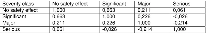
A probability function is sought for the number which indicates how the number of occurrences in separate severity classes are related each other. This number is given as the ratio of the number of occurrences in two severity classes. In order to find a distribution for this ratio it is necessary to deter-mine whether the number of aircraft involved with occurrences in severity classes have a dependency. Thus, the correlation between the severity classes is determined with Pearson’s correlation coefficient. The strength of correlation between the number of occurrences in severity classes is determined by the value of the correlation-coefficientρ:

Definition 7.3.1 (Strength of correlation). The strength of the correlation is based on the correlation-coefficientρand is determined as follows:

[0.0 - 0.2] Negligible correlation [0.2 - 0.4] Weak correlation [0.4 - 0.6] Reasonable correlation [0.6 - 0.8] Strong correlation [0.8 - 1.0] Very strong correlation

Whenρis negative, there is a negative correlation.

The strength of a correlation between variables indicates (statistical) (in)dependency. Weak or neg-ligible correlation suggests independence, where stronger correlations suggest dependence.

Assumption 7.3.2 (Dependency based on correlation coefficients). Variables are assumed (statisti-cally) independent when the correlation is negligible or weak.

(31)

Proposition 7.3.3 (Distribution for the ratio of two Poisson variables). Given X ∼ P oisson(λx) and

Y ∼P oisson(λy), whereX andY are independent. The probability distribution for the ratioR= X_Y is:

PnX Y ≤t

o =

∞

X

n=0

e−λy_λn

y

n! e

−λx btnc

X k=0 λk x k! Proof:

PnX Y ≤t

o

= P{X ≤Y t}

= P{X ≤Y t|Y =n} ·P{Y =n}

= P{X ≤tn} ·P{Y =n}(use independence) =

∞

X

n=0

btnc

X

k=0

e−λx_λk

x

k!

e−λy_λn

y n! = ∞ X n=0

e−λy_λn

y

n! e

−λx btnc

X

k=0

λk_x k!

An analytic derivation of the distribution function for the ratio of two dependent Poisson distributed variables by using the Poisson distribution function is not possible. Thus, the distribution for the ratio is determined empirically with its mean and variance.

This is done by determining the ratio of the number of aircraft involved with occurrences between sever-ity classes for each month, followed by determination of the average value of the ratio and its variance. Note: as division by zero is impossible, the empirical distribution cannot be determined if one or more months of the severity class which is used as denominator has zero occurrences. Thus:

Definition 7.3.4(Empirical distribution for the ratio of dependent variables). The empirical distribution of the ratioR= X_Y of two variablesXandY is determined by its mean and variance:

EhX Y i = 1 n n X i=0 xi yi

V arX Y = 1 n n X i=0 x_i yi 2 − 1 n2 Xn i=0 xi yi 2

(32)

(33)

Chapter 8 Numerical results

The numerical analysis of the model exists of the numerical results from the mathematical methods used. This starts by using the test of Kolmogorov-Smirnov to determine if the Poisson distribution is applicable, this is performed in section 8.1. Next two case studies are presented in which Poisson regression is carried out to determine estimators for the average number of aircraft involved with oc-currences for the combinations of states of the factors. This is first done for the type of occurrence called ’deviation taxi’ in section8.2, which is chosen because LVNL has particular interest in this type. Next section8.2looks at major incidents, which is chosen because it is an important severity class for risk-analysis at LVNL. Last section8.3determines the correlation coefficients for the severity classes, which helps to determine the distribution for the earlier described ratio for the number of occurrences in the severity classes.

8.1 Performing statistical tests

This section gives the distribution found for each type of occurrence and for each severity class for the number of aircraft involved with occurrences by using the test of Kolmogorov-Smirnov. The tested Poisson parameter is the sample average for each case. The Poisson distribution is assumed when the significance valueαis larger than the confidence levelα0, the confidence level used is 5%; thus reject

the Poisson distribution whenα <0.05.

Poisson distributions for the types of occurrences

For performing the Kolmogorov-Smirnov test the data is collected per month, as shown in tableB.1in appendixB.1. In tableD.1the results are shown for the type of occurrences i∈ _I(column 1), where the second column gives the Poisson parameter and the third column gives the significance value. The Poisson distribution is assumed to be correct if the significance value is greater than or equal toα. The test-results show that all types of occurrencesi have a Poisson distribution, except for ’Airspace infringement’, ’Apron incursion incident including pushback incident’, ’Deviation Startup pushback’, and ’Deviation Vehicle - airport traffic’. These categories are studied more closely.

Looking at the latter three types, it is known that there were only few reports before February 2011, and that there are more occurrences reported after. This can be explained by the fact that an aware-ness meeting has been held to emphasize the importance of reporting occurrences, the increase on the number of occurrences is visible from this moment on. Looking for the distribution of these types of occurrences after the awareness meeting, the test indicates that a Poisson distribution is applicable. The results are displayed in tableD.2.

Looking at ’Airspace Infringements’, a clear seasonal pattern is visible in the number of occurrences per month. In [11] it is already shown that the number of occurrences heavily depends on the IATA sea-sons, which is defined as the dates which have ’summertime’ and those which have ’wintertime’. This is explained by the fact that uncontrolled traffic from the smaller fields which are close to Schiphol airport and are not under the responsibility of LVNL cause airspace infringements. The amount of this type of traffic is considerably larger during the summer months. Thus, the number of occurrences are regarded during the summer- and winter-months are tested separately. The split seasons have a Poisson distri-bution, with their corresponding sample mean as Poisson parameter. The results are displayed in table

(34)

Poisson distributions for the severity classes

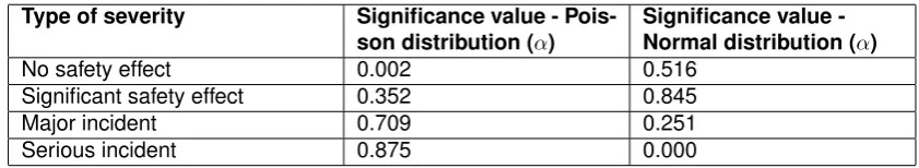
It is known from [11] that the occurrences in several severity classes are normally distributed. This study is interested in the Poisson distribution. Thus, the Kolmogorov-Smirnov test is performed for both the Poisson and the normal distribution. Since they resemble each other when the means increases, the results of the tests are compared. The Poisson distribution is more likely to be applicable when the average number of aircraft involved with occurrences is low and the mean is equal to the variance. The normal distribution is more likely to be applicable when the average number of aircraft involved with occurrences is high and there is overdispersion; which means that the mean and variance are not equal. Both the Poisson and the normal distribution are tested. The results of the tests are shown in table

8.1, now only the significance level (α) is shown for sake of clarity; again when the significance level is equal to or greater thanα0(= 0,05) the tested distribution is accepted. The results show that the

severity class ’no safety effect’ has a normal distribution (with mean40) and not a Poisson distribution. An explanation for this is that the average number of occurrences per month is relatively high and there is overdispersion.

The severity class ’serious incident’ has a Poisson distribution (with mean0.47) and not a normal dis-tribution, this can be explained by the fact that the average number of occurrences per month is low. The severity classes ’significant safety effect’ and ’major incident’ (with resp. mean11and3) can be assumed to have both a normal and a Poisson distribution. This result is explained by the fact that the Poisson and normal distribution resemble each other as the mean number of occurrences per month increases, and there is no overdispersion.

Type of severity Significance value - Pois-son distribution (α)

Significance value -Normal distribution (α)

No safety effect 0.002 0.516

Significant safety effect 0.352 0.845

Major incident 0.709 0.251

[image:34.595.86.507.305.382.2]

Serious incident 0.875 0.000

Table 8.1: Output Kolmogorov-Smirnov - Severity classes

8.2 Performing Poisson regression: case studies

This section illustrates two case studies regarding the determination of estimators for the average num-ber of aircraft involved with occurrences per movement for combinations of states of factors by Poisson regression. Poisson regression is first performed for type of occurrence ’deviation taxi’, next it is per-formed for severity class ’major’. The results on the estimated rates are shown here, the use of these results for identifying factors which contribute to risk is shown in section9.2.

The progress of obtaining results of Poisson regression in SPSS is stated in appendixB.2. For sake of clarity only the final results of Poisson regression are shown, detailed results can be found in appendix mentioned.

Case study - Factors influencing types of occurrences: Deviation taxi

This case study describes the results of Poisson regression for the type of occurrence called ’deviation taxi’; this type is defined as ’deviation of the instructed or according to the regulations applicable proce-dure for taxiing’.

(35)

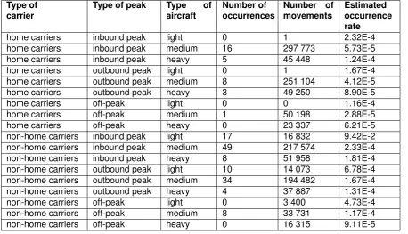
In determining the estimators for the parameters, a selection of the states of the factors is chosen as a ’reference setting’. In this case: non-home carriers (X0,1) during the off-peak (X0,2) with light aircraft

(X0,3). The estimators for these parameters are set zero. The remaining variables are defined as:

- Type of carrier:X1= 1in case of home carriers, elseX1= 0

- Type of peak:X2= 1in case of inbound peak, elseX2= 0

- Type of peak:X3= 1in case of outbound peak, elseX3= 0

- Type of aircraft:X4= 1in case of heavy aircraft, elseX1= 0

- Type of aircraft:X5= 1in case of medium aircraft, elseX1= 0

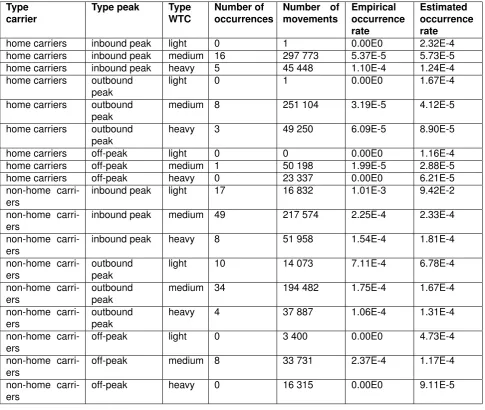
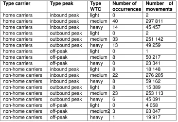
The choice of these factors results in 18 combinations with in total 163 occurrences for Deviation Taxi. To get a correct view on the effects of (the combinations of) factors, the occurrences corresponding to the chosen circumstances are counted. The number of occurrences and the number of movements is given for each combinations of states of factors in table8.2.

The initial model equation of Poisson regression is:

lnµi Vi

= β0+β1·X1+β2·X2+β3·X3+β4·X4+β5·X5

+γ1,2·X1•X2+γ1,3·X1•X3+γ1,4·X1•X4+γ1,5·X1•X5+γ2,3·X2•X3

+γ2,4·X2•X4+γ2,5·X2•X5+γ3,4·X3•X4+γ3,5·X3•X5+γ4,5·X4•X5

The test performed than has the null-hypothesis βi = 0andγj,l = 0, and the alternative hypothesis

βi 6= 0andγj,l6= 0, so:

H0:βi= 0, γj,l= 0,∀i, j, l; H1:βi6= 0, γj,l6= 0,∃i, j, l

Now for each factor it is first determined if the effect they have on the number of aircraft is observ-able, which is indicated by the significance value. The significance value is determined by Wald’s test, as described in appendixA.3; again significance levelα0= 0,05is assumed.

Following the progress as stated in appendixB.2: the null-hypothesis is not rejected for thoseβand

γwhich have a significance value which is bigger thanα0. Thus, these have value zero and are deleted

from the model equation one-by-one; their influence is not observable.

Deleting the non-significant variables one-by one leads to the following results:

First: the significance value is 0.000 for the factors ’type of carrier’ and the ’type of aircraft’, it is 0.036 for ’type of peak’. This means all factors have an observable influence on the number of occurrences of type ’deviation taxi’ and thus remain in the model equation.

Second: looking at the interaction-terms, only the interaction between home carriers with heavy aircraft is significant and thus remains in the model equation.

The model equation becomes:

lnµi Vi

= β0+β1·X1+β2·X2+β3·X3+β4·X4+β5·X5+γ1,3·X1•X3

The estimators ofβi andγj,l are determined as:

β0=−7.953

β1=−1.323 β2= 0.923 β3= 0.565 β4=−1.984

β5=−1.537

γ1,3= 1.018

Whereβ0 represents the estimator for the reference setting (non-home carriers during the off-peak

with light aircraft),β1represents the estimator for home carriers,β2andβ3the estimators for resp. the

inbound- and outbound-peak,β4andβ5 for resp. heavy and medium aircraft. Further,γ1,3represents

Model development for supporting advanced risk based approaches in air traffic management

MODEL

DEVELOPMENT

FOR

SUPPORTING

RISK-BASED

APPROACHES

CENSORED

Summary

Contents

List of abbreviations

Chapter 1

Preface

Chapter 2

Background, introduction problem,

goals

2.1

Background

2.2

Introduction to problem

2.3

Goals

Chapter 3

Literature review

Adjacent fields

Methods for investigating statistical characteristics

Difficulties in (supporting) risk-based approaches

Chapter 4

Available data and its structure

4.1

Types of occurrences

4.2

Severity classification

Chapter 5

Assumptions

Chapter 6

Model

6.1

Description of the model

6.2

Main elements of the model

6.3

Relations between and in the main elements of the model

Chapter 7

Analysis

7.1

Practicability of reference values

7.2

Determination of risk-contributing factors

7.3

Relation severity classes

Chapter 8

Numerical results

8.1

Performing statistical tests

8.2

Performing Poisson regression: case studies