Bivariate stochastic modeling of functional response with natural mortality

University of Warwick institutional repository: http://go.warwick.ac.uk/wrap

This paper is made available online in accordance with publisher policies. Please scroll down to view the document itself. Please refer to the repository record for this item and our policy information available from the repository home page for further information.

To see the final version of this paper please visit the publisher’s website. Access to the published version may require a subscription.

Author(s): M. J. Faddy, J. S. Fenlon and D. J. Skirvin

Article Title: Bivariate Stochastic Modeling of Functional Response With Natural Mortality

Year of publication: 2010 Link to published version:

http://dx.doi.org/ 10.1007/s13253-009-0007-9

Bivariate stochastic modelling of functional response with natural

mortality

M.J. FADDY, J.S. FENLON and D.J. SKIRVIN

A correction due to Abbott (1925) is the standard method of dealing with control mortality in insect bioassay to estimate the mortality of an insect

conditional on control mortality not having occurred. In this paper a bivariate stochastic process for overall mortality is developed in which natural mortality and predation are jointly modelled to take account of the competing-risks

associated with prey loss. The total mortality estimate from this model is essentially identical with that from more classical modelling. However, when

predation loss is estimated in the absence of control mortality the results are somewhat different, with the estimate from the bivariate model being lower than that from using Abbott’s formula in conjunction with the classical model.

It is argued that over-dispersion in observed mortality data corresponds to correlated outcomes (death or survival) for the prey initially present, while

Abbott’s correction relies implicitly on independence.

Keywords: Stochastic modelling; Competing risks; Estimation of predator

mortality; Over-dispersion. ________________________

M.J. Faddy is Adjunct Professor, School of Mathematical Sciences, QUT, Brisbane, Qld 4000, Australia. J.S. Fenlon is Reader, Department of Statistics, University of Warwick,

Coventry, CV4 7AL, England ([email protected]), previously at Horticulture

Research International, Wellesbourne, CV35 9EF, England. D.J. Skirvin is Senior Research

1 INTRODUCTION

It is often the case in bioassays that mortality of insects can occur for reasons other than those due to the substance under investigation. Morgan (1992) makes the distinction

between ‘natural’ and ‘control’ mortality, citing Hoekstra (1987) and Preisler (1989). Natural mortality may occur as well as mortality due to handling of the insects, or mortality

may be due to the fact that the insects are not in their natural habitat. In order to assess the degree of ‘control mortality’, groups of insects are often kept under conditions that are the same as those for the treated groups, except for the absence of the treatment. Abbott’s

formula (Abbott, 1925) is then commonly used to estimate treatment mortality in the absence of control mortality for dose response assays. For a given dose d, if the expected

proportion responding is p then this is not directly observable because of contamination through natural mortality; so if the expected overall proportion dead is p*, then p* is made up of the proportion of insects φ that die naturally, and a proportion p of the remainder

(1 – φ) that die due to the treatment, so that p* = φ + (1‒φ)p. The actual probability of

dying because of the dose is therefore given by p = (p*‒φ)/(1‒φ). Hewlett and Plackett

(1979) remark that it is rarely possible to test the assumptions on which this formula is based, and cite Kuenen (1957). They make the rather surprising comment that “control

response should be avoided if possible”.

A particular type of assay in predator-prey studies, known as a functional response assay, involves experiments in which different numbers of prey are made available to a single predator (see, e.g. Fenlon and Faddy, 2006). The data presented here derive from a

simulation models to examine practical biological control scenarios (Skirvin et al. 2002). However, in moving to larger arenas it was not possible to guarantee recovery of

non-predated prey, so that a simultaneous assay procedure was used with separate arenas for control and predator groups. Classical models with beta-binomial distributed residuals about

a mean function, as described in Fenlon and Faddy (2006), are first fitted to the data, with predator mortality estimated using Abbott’s formula. The main contribution of the paper is the development of a bivariate stochastic process model for both predation loss and natural

mortality as an extension of the univariate stochastic model in Fenlon and Faddy (2006), and the fitting of this model to the data. This bivariate modelling owes its genesis to a recent

paper by Faddy and Smith (2005). Estimates of predator mortality in the absence of control mortality from the classical and stochastic modelling approaches are then compared, and the paper concludes with some speculations on the reasons for the apparent differences between

these estimates.

2 DATA

Details of the experimental procedure are given in Skirvin and de Courcy Williams (1999) and Skirvin and Fenlon (2001). The assay system comprised cut stems with four tri-foliate leaves of Choisya ternata (a popular garden ornamental sometimes called Mexican orange

blossom). Mini-plants were ‘primed’ with webbing of the spider mite Tetranychus urticae, a pest of many garden plants, before elimination of all life stages of the spider mite.

Different levels of pest load were then transferred to individual stems using a fine

paintbrush, and a single Phytoseiulus persimilis (predator) was introduced onto each stem before the stems were placed in individual perspex cylinders which were sealed with

initially) with the predator present varied (average 19), and there were 25 control assays with 40 prey initially, in which no predator was present, to monitor natural loss(es).

For each individual assay the number of surviving prey was counted after 24 hours, and the

number predated or lost determined by difference. Data from assays in which the predator was not found, or was dead, were excluded. Similarly, control assays in which a predator was found were also removed from the analysis. The data with some summary statistics are

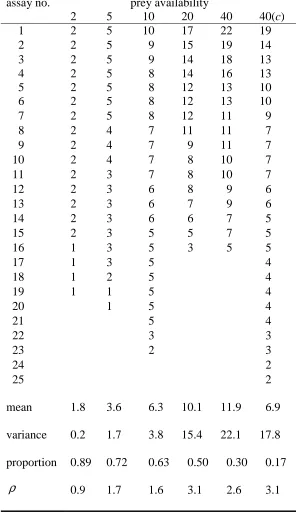
presented in Table 1 and plotted in Figure 1. With the exception of availability level 2, it appears that all these data show over-dispersion relative to the binomial distribution, with

the over-dispersion tending to increase with prey availability (the variance ratio statistics in the final row of Table 1 bear this out).

3 CLASSICAL MODELLING

3.1 BETA-BINOMIAL MODEL

In the summaries of the data it is quite clear that simple binomial modelling is really of no value since over-dispersion relative to the binomial distribution is significant. So, a beta-binomial (residual) distribution was used:

P(n prey lost) =

(

)

(

, ,

)

N

N N

N

N N

B n N n

N

n B

µ µ

θ θ

µ µ θ θ

−

−

+ − +

     

where (. , .)B is the beta function. The mean of this distribution is µ and the variance

( )

1 N 1

( )

1

(

N 1

)

µ θ

θ

the compound data (predation with natural mortality) was modelled as a function of the availability N, with some adjustment being made for natural (or control) mortality using

Abbott’s formula. The underlying model then takes the form:

ϕ

µ

control =N (1)

and

µ

_compound =N

ϕ

+ −

(

1

ϕ µ

)

_predator (2)

where µcontrol, µcompound and µpredator correspond to the means for the respective subscript

groups. Only data relating to the control and compound means are observable, with the predator mean being inferred. As in Fenlon and Faddy (2006) µpredator is modelled using a

Gompertz function constrained to pass through the origin:

(

)

[ ]

{

exp exp exp

}

predator a b cN b

µ

= _− − _− − (3)

which corresponds to a Type III functional response model (Holling, 1959). Some additional modelling of the over-dispersion parameter θ as a function of N was indicated by the data –

the details are deferred to the next sub-section.

3.2 RESULTS

A saturated beta-binomial model was first fitted to the control and compound data by

maximum likelihood; this consisted of individual two-parameter beta-binomials for each prey availability level, N. It was noted that estimates of the beta-binomial over-dispersion parameter, θ, generally declined with prey availability, so several forms were tried, with

means from equations (1), (2) and (3), to describe the control and compound data over all availability levels:

(a) θ = d,

(b) θ = d0 for control data, and θ = d1 for the compound data,

(d) θ = d0 for control data, and θ = d1 + e/N for the compound data.

All fits resulted in large estimated a’s and small b’s in the form of µpredator given by (3),

corresponding to the limiting (a →∞ and b → 0 with ab=a′) form:

µ_predator =a′_1 exp−

(

−cN

)

_, (4)

with a′ and c>0; i.e., type II behaviour without an inflexion point (Holling, 1959). The

respective log-likelihoods from the model fits were −249.0, −248.5, −248.3 and −248.2, and the corresponding AIC values (−2 × {log-likelihood − no. of parameters}) 505.9, 507.0,

506.6 and 508.4, which all suggest that staying withthe simplest model (a) is not unreasonable.

However, the corresponding generalised Pearson statistics (sums of squared standardised residuals), which give measures of goodness of fit, were 125.8, 123.9, 118.9 and 119.4 with

115, 114, 114 and 113 d.f., respectively. These show quite a marked reduction when θ is made dependent on N, and suggest that a model based on (c) might be preferred, with the generalised Pearson statistic indicating a better fit. Such a decline in θ with N does moderate

the dispersion for larger N, more in accord with the values in Table 1. This model also compares favourably with the saturated model (deviance = 5.3 on 7 d.f.). The fit of the

model to the compound (predator + control) mortality data is illustrated in Figure 1 where the estimated mean from (2) and (4) is plotted with ± one standard deviation limits. The fit to the control data gave estimated mean 6.8 and variance 16.2, compared with the observed

values of 6.9 and 17.8 shown in Table 1. The most extreme observation is the count of 19 in this control data sub-set, and corresponds to a tail probability of just under 0.01, which

estimated under the assumption that a beta-binomial distribution applies with the same over-dispersion parameter as that associated with the compound mortality.

4 STOCHASTIC PROCESS MODELLING

4.1 BIVARIATE STOCHASTIC MODEL

In Fenlon and Faddy (2006) probability distributions on 0, 1, …, N for the number of prey

lost were constructed from a univariate Markov process

{

X t t

( )

; ≥0

}

with X

( )

0 =0 and

rate parameters λ0, λ1, …, λN–1, λN (with λN = 0) where:

(

)

( )

{

}

P X t+

δ

t = +n 1|X t =n =

λ δ

n t.

The modelling of prey loss is here extended to a bivariate Markov process

( ) ( )

{

X t Y t t, ; ≥0 ,

}

with one component X(t) for natural mortality and the other Y(t) for

predator mortality, with 0 ≤ X(t)+ Y(t) ≤ N and X(0) = Y(0) = 0. So that two transitions now have to be considered, with infinitesimal probabilities:

and

{

(

)

(

)

}

(

)

(

)

{

}

(1)

(2)

P 1, | ( ) , ( )

P , 1 | ( ) , ( )

x y

x y

X t t x Y t t y X t x Y t y t

X t t x Y t t y X t x Y t y t

δ δ λ δ

δ δ λ δ

+ = + + = = = =

+ = + = + = = = (5)

representing, respectively, an increase in the natural mortality of the prey, and an increase in predator-induced mortality. Whilst X(t) can be observed Y(t) cannot; what is observed, rather, is the total mortality X(t)+ Y(t). However, since the processes may not be

independent, the rates

λ

_{x y}(1) of natural mortality and

λ

_{x y}(2) of predator mortality cannot simply

The solution for the probabilities p x y( , )=P

{

X

( )

1 =x Y,

( )

1 = y

}

where the process of prey

loss is taken, without loss of generality, to run for one unit of time can be expressed in terms of a matrix, Q, of transition rates from (5). The rows and columns of this matrix are indexed

by

( )

x y, taking the values

( ) ( ) (

0,0 , 0,1 ,…, 0,N

) ( ) ( ) (

; 1,0 , 1,1 ,…, 1,N −1 ;

) (

…; N,0

)

with the

three non-zero elements of Q in the row corresponding to

( )

x y, being:

(

(1) (2)

)

x y x y

λ λ

− + in the column corresponding to

( )

x y, ,

(1)

x y

λ

in the column corresponding to

(

x+1,y

)

, and

(2)

x y

λ

in the column corresponding to

(

x y, +1 ,

)

except when x+ y = N in which case all the entries are zero. The probability p x y

( )

, is then

the appropriate element in the row vector (cf. Fenlon and Faddy, 2006):

( ) ( )

(

) ( ) ( )

(

)

(

)

[

]

( )

0,0 0,1 0, 1, 0 1,1 1, 1 , 0

1 0 0 exp ,

p p p N p p p N − p N

    = … … … ⋯ Q (6)

with the probability of a total of n prey lost then given by the convolution

(

)

0 , ,

n

x= p x n−x

∑

for n=0,1,…, N.

A reasonable description of control mortality would be in terms of the total numbers lost,

i.e.

λ

_{x y}(1) = f x

(

+y

)

. For predation mortality, following Fenlon and Faddy (2006), a product

form is used where

λ

_{x y}(2) =g y h x

( ) (

+ y

)

; here g(y) can be thought of as a predator

behaviour component [e.g. g(y) constant would correspond to constant predator activity regardless of the number of prey consumed] and h(x+y) as relating to the prey [e.g.

h(x+y) = N–x–y would correspond to the remaining prey being exchangeable (Faddy and

Fenlon, 1999)]. The expression:

corresponds to a simple binomial distribution with probability φ for control mortality in the absence of predator mortality. And, following Fenlon and Faddy (2006), the form

(2)

(

)

{

(

)

}

1 exp ( )

exp

x y

N x y

y

ε

δ

λ α β

δ

 _{− − − +} 

 

= + (8)

was used, which, for β > 0, corresponds to greater predator activity with increasing prey

consumed and, for δ > 0 and/or ε≠ 1, non-exchangeable prey.

4.2 RESULTS

The bivariate stochastic process model for both control and predator mortality described by

the transition rates in equations (5) and the probabilities from (6) with the expression (7) for

(1)

,

λ as has already been remarked, corresponds to a simple binomial distribution with

probability φ for control mortality in the absence of predator mortality. However, the analysis of section 3.2 showed that the control mortality exhibited over-dispersion relative

to the binomial distribution, and that a beta-binomial distribution was more appropriate. Beta-binomially distributed control mortality can be incorporated into the bivariate

stochastic process with the probability of x prey lost naturally and y lost by predation being given by:

(

)

(

)

( )

1 1 1 0 1 , | , , s r

p x y d

r s

ϕ

ϕ

ϕ

ϕ

− − ₋ Β

∫

(9)

where p x y

(

, |

ϕ

)

is the probability of x prey lost naturally and y prey lost by predation for a

given value of φ, determined from equations (6), (7) and (8), and the other component in the

integrand of (9) is the probability density function of a beta distribution.

Use of probabilities given by equation (9) is very costly in computing time, as numerical

large matrices (6); to expedite these computations a discrete binomial mixture distribution for control mortality was used as an alternative. A discrete mixed binomial model uses

probabilities

(

)

1 , , ,

k

i i

i= w b N

ϕ

x

∑

where 0≤wi ≤1, ₁ 1

k

i i= w =

∑

and 0≤ ≤

ϕ

_i 1 for i=1,2,…, k,

k being the number of components in the mix, and b N

(

, _i,x

)

N _ix

(

1 _i

)

N x, x

ϕ

₌ 

ϕ

₋

ϕ

−

 

 

0≤ ≤x N, are binomial probabilities. Table 2 shows details of maximum likelihood fitting

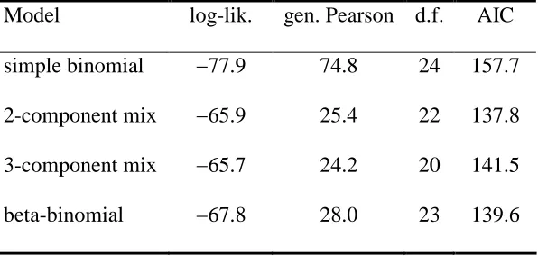
of these distributions to the control data: a two component binomial mixture model would be selected according to the AIC values, and it shows a fit to the data that is comparable to the beta-binomial.

Fitting the bivariate stochastic process model with a two component binomial mixture

distribution for the control mortality simply involves probabilities p x y

(

, |

ϕ

₁

)

and

(

, | 2

)

p x y

ϕ

created from only two matrices Q1 and Q2 derived from equations (6), (7) and

(8) with probabilities φ1 and φ2, respectively, and using the discrete version of expression (9):

(

) (

) (

)

1 , | 1 1 1 , | 2 .

w p x y

ϕ

+ −w p x y

ϕ

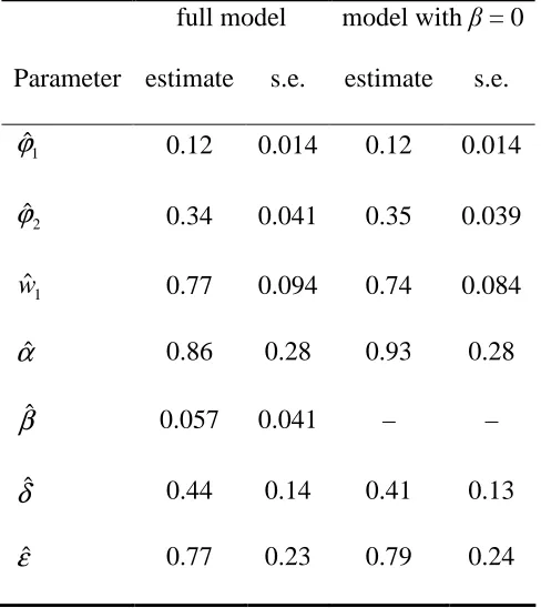
Parameter estimates and their corresponding standard errors from fitting this model to the control and compound mortality data are given in the second and third columns of Table 3. The log-likelihood under this model is –245.4, compared to −248.3 from the previously

fitted beta-binomial model. However, these two models have different sub-models (two-component mixed binomial and beta-binomial, respectively) for the control data, and the

The results in Table 3 suggest that setting β = 0 in equation (8), corresponding to constant predator activity, might be acceptable, and indeed, fitting such a reduced model results in

only a small decline in the log-likelihood from –245.4 to –246.0. However, the overall generalised Pearson statistic increases from 114.6 on 112 d.f. to 125.1 on 113 d.f. when

β = 0, indicating a poorer fit, and the latter model seems less convincing for the data

corresponding to N = 5 and 20. Exceedance probabilities of apparent outliers for the full (β > 0) model correspond to one with tail probability about 0.01 and three with tail

probabilities between 0.01 and 0.05, which would seem unremarkable given the size of the data-set.

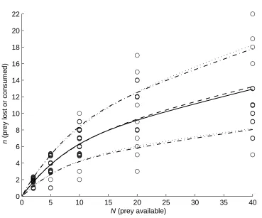
Shown in Figure 1 is the estimated mean total mortality from the full (β > 0) model (along with the data and estimated means from the previously fitted beta-binomial model); the

figure also shows the spread of ± one standard deviation about the mean for both models. These two fits are clearly very similar. The estimated mean control mortality was 6.8,

similar to the earlier fitted beta-binomial value, but the estimated variance was slightly larger at 19.0 (cf. 16.2) so that the 2-component mixed binomial distribution used here is somewhat better able to accommodate the extreme count of 19 in the control data sub-set.

The estimated predation when natural mortality is not present can be determined from the

distribution of Y(1) corresponding toλ(1) ≡0in (5), and is shown in Figure 2 (along with that from the beta-binomial model); the ± one standard deviation limits here have been

5 DISCUSSION

The main contribution of this paper has been the construction of a bivariate stochastic process model for natural and predator mortality, and the comparison of the results from fitting this model to a data-set with those from a more classical approach. The

differentiation methods used to estimate net predation for the two models in the absence of natural mortality gave rather different results: the stochastic process model used the

univariate process with the natural mortality transition rates set to zero, whereas the beta-binomial modelling used Abbott’s formula. This resulted in rather different estimates, with those from the stochastic model being lower than those from the beta-binomial (Figure 2),

even though the estimates of total mortality were virtually identical (Figure 1). While both mean responses and the standard deviation from the stochastic process model have stabilised

by N = 40, the standard deviation from the beta-binomial model continues to increase; however, the assumption under which this has been estimated, i.e. that the level of over-dispersion is the same as that for total mortality, is clearly unverifiable. An aesthetic

argument can be made for the stochastic process modelling which has a consistency insofar as the ‘tension’ between the control and compound mortality (with the former sometimes

outrunning the latter for large N) leads to an early horizontal asymptote of the compound mortality (effectively satiation) within the experimental range. Furthermore, the stochastic modelling attempts to model the actual temporal process of predation, and offers a possible

explanation of how the predator behaves in relation to changing prey availability, even though the data are observed only at a single time point. The problem associated with

over-dispersion in the control data has been addressed in the stochastic modelling by the use of a discrete binomial mixture model to obviate the need for costly numerical integration

involving many matrix exponential evaluations associated with using a beta-binomial

Abbott’s formula essentially estimates for an individual prey the conditional probability of

loss due to the predator given that natural death has not occurred, where predator and natural mortality can be considered as competing risks. A more appropriate estimate is that of the

unconditional probability of loss due to the predator. These probabilities will be the same if

the risks of predator and natural mortality are assumed to apply independently to the prey. A further assumption that loss (either natural death or death from predation) occurs

independently between prey when there are several available initially will lead to a binomial distribution of the number of prey lost during the course of an experiment or study, with

Abbott’s formula giving an estimate of the unconditional mean number of prey lost to the predator.

However, if the observed number of prey lost shows residual variation in excess of that corresponding to binomial variation then both the above assumptions of independence are

called into question. Extra-binomial variation in numbers lost can be explained either by a residual distribution that shows over-dispersion (such as the beta-binomial) or a stochastic process running during the course of the experiment with rates of loss of individual prey that

are not constant but a function of the accumulating number of prey lost. In both of these models, the over-dispersion corresponds to correlated outcomes (death or survival) for the

initial number of prey. And there is an equivalence between these models in that any

distribution showing over-dispersion relative to the binomial has a representation in terms of a stochastic process with varying rates of individual prey loss (Faddy, 1997) – some

increase in these rates with the accumulating number of prey lost gives rise to the over-dispersion. Such a stochastic representation of predator mortality will result in the two

would be exposed to higher rates of predation than those that might die earlier, since more prey are likely to be consumed by the predator in a longer period of time. So Abbott’s

formula, which (generally) leads to an estimate of the mean number of prey lost to the predator conditional on natural death not occurring, will not give an estimate of the

unconditional mean number of prey lost to the predator because of this dependence between natural and predator mortality. However, the bivariate stochastic model of predator and natural mortality will give an estimate of this unconditional mean number of prey lost to the

predator if the natural mortality component of the model is set to zero.

There is no doubt that there are challenges in modelling these data, and deriving estimates of predator mortality. Further models may be developed, but what has been presented here does offer a novel approach to the problem and a very plausible estimate of net predation,

with interpretable dynamics. The use of stochastic process modelling ultimately provides an appropriate temporal structure giving a reasonable explanation for observed data on

functional response, as has been previously argued in Fenlon and Faddy (2006).

ACKNOWLEDGEMENTS

The authors wish to express their thanks and appreciation to the reviewers for the many

REFERENCES

Abbott, W.S. (1925), “A method for computing the effectiveness of an insecticide”, Journal of Economic Entomology, 18, 265−267.

Faddy, M.J. (1997), “Extended Poisson process modelling and analysis of count data”, Biometrical Journal, 39, 431−440.

Faddy, M.J. and Fenlon, J.S. (1999), “Stochastic modelling of the invasion process of nematodes in fly larvae”, Applied Statistics, 48, 31−37.

Faddy, M.J. and Smith, D.M. (2005), “Modelling the dependence between the number of

trials and the success probability in binary trials”, Biometrics, 61, 1112−1114.

Fenlon, J.S. and Faddy, M.J. (2006), “Modelling predation in functional response”,

Ecological Modelling, 198, 154−162.

Hewlett, P.S. and Plackett, R.L. (1979), The Interpretation of Quantal Responses in Biology, London: Edward Arnold.

Hoekstra, J.A. (1987), “Acute bioassays with control mortality”, Water, Air and Soil Pollution, 35, 311−317.

Kuenen, D.J. (1957), “Time mortality curves and Abbott’s correction in experiments with insecticides”, Acta Physiologica et Pharmacologica Neerlandica, 6, 179–196.

Morgan, B.J.T. (1992), Analysis of quantal response data, London: Chapman & Hall.

Preisler, H.K. (1989), “Fitting dose-response data with non-zero background within generalized linear and generalized additive models”, Computational Statistics and Data

Analysis, 7, 279−290.

Skirvin, D.J. and de Courcy Williams M. (1999), “Differential effects of plant species on a mite pest (Tetranychus urticae) and its predator (Phytoseiulus persimilis): implications for biological control”, Experimental and Applied Acarology, 23, 497−512.

Skirvin, D.J. and Fenlon. J.S. (2001), “Plant species modifies the functional response of

Phytoseiulus persimilis (Acari: Phytoseiidae) to Tetranychus urticae (Acari: Tetranychidae):

implications for biological control”, Bulletin of Entomological Research, 91, 61−67.

Skirvin, D.J., de Courcy Williams, M.E., Fenlon, J.S. and Sunderland K.D. (2002), “Modelling the effects of plant species on biocontrol effectiveness in ornamental nursery

[image:18.595.141.437.189.706.2]

Table 1: observed numbers and summary statistics of T. urticae adults consumed or lost (with predator) and control c (without predator) for groups of assays with the same prey

availability; ρ is the ratio of sample to binomial variance (a measure of over-dispersion).

assay no. prey availability

2 5 10 20 40 40(c)

1 2 5 10 17 22 19

2 2 5 9 15 19 14

3 2 5 9 14 18 13

4 2 5 8 14 16 13

5 2 5 8 12 13 10

6 2 5 8 12 13 10

7 2 5 8 12 11 9

8 2 4 7 11 11 7

9 2 4 7 9 11 7

10 2 4 7 8 10 7

11 2 3 7 8 10 7

12 2 3 6 8 9 6

13 2 3 6 7 9 6

14 2 3 6 6 7 5

15 2 3 5 5 7 5

16 1 3 5 3 5 5

17 1 3 5 4

18 1 2 5 4

19 1 1 5 4

20 1 5 4

21 5 4

22 3 3

23 2 3

24 2

25 mean variance proportion ρ 2

1.8 3.6 6.3 10.1 11.9 6.9 0.2 1.7 3.8 15.4 22.1 17.8 0.89 0.72 0.63 0.50 0.30 0.17

[image:19.595.128.426.155.297.2]

Table 2: log-likelihood, generalised Pearson and AIC statistics for mixed binomial models in comparison to the beta-binomial model for the control data.

Model log-lik. gen. Pearson d.f. AIC

simple binomial

2-component mix 3-component mix

beta-binomial

−77.9

−65.9 −65.7

−67.8

74.8

25.4 24.2

28.0

24

22 20

23

157.7

137.8 141.5

[image:20.595.156.400.128.402.2]

Table 3: parameter estimates of the bivariate stochastic process model of natural mortality and predator mortality.

full model model with β = 0 Parameter estimate s.e. estimate s.e.

1

ˆ

ϕ 0.12 0.014 0.12 0.014

2

ˆ

ϕ 0.34 0.041 0.35 0.039

1

ˆ

w 0.77 0.094 0.74 0.084

α_ˆ 0.86 0.28 0.93 0.28

βˆ _{0.057 0.041 – –}

δ

ˆ _{0.44 0.14 0.41 0.13}

0 5 10 15 20 25 30 35 40 0

2 4 6 8 10 12 14 16 18 20 22

N (prey available)

n

[image:21.595.115.484.76.383.2]

(prey lost or consumed)

Figure 1: estimates of mean total prey lost or consumed from the bivariate stochastic process model (——) and the beta binomial model (− − −); ± one standard deviation limits are

0 5 10 15 20 25 30 35 40 0

2 4 6 8 10 12

N (prey available)

n

[image:22.595.117.476.90.385.2]

(net prey consumed)

Figure 2: estimates of mean net prey consumed by the predator from the bivariate stochastic process model (——) and the beta binomial model (− − −); ± one standard deviation limits