University of Warwick institutional repository
This paper is made available online in accordance with
publisher policies. Please scroll down to view the document
itself. Please refer to the repository record for this item and our
policy information available from the repository home page for
further information.
To see the final version of this paper please visit the publisher’s website.
Access to the published version may require a subscription.
Author(s): Francesca M. Poli, Sergei E. Sharapov
and JET-EFDA
contributors
Article Title: A wavelet-based method to measure the toroidal mode
number of ELMs
Year of publication: 2009
Link to published version:
A wavelet-based method to measure the toroidal mode number of
ELMs
Francesca M. Poli
1), Sergei E. Sharapov
2)and JET-EFDA contributors
a) JET-EFDA, Culham Science Centre, OX14 3DB, Abingdon, UK1)University of Warwick, Coventry CV4 7AL, UK 2)EURATOM/UKAEA Fusion Assoc., Abingdon OX14 3DB, UK
a)See the Appendix of F. Romanelli et al., Fusion Energy 2008 (Proc. 22nd Int. Conf. Geneva, 2008) IAEA, (2008)
The high confinement mode regime (H-mode) in tokamaks is accompanied by the occurrence of burst of MHD activity at the plasma edge, so-called edge localized modes (ELMs). Because of the short time scales involved in the ELM crash (on JET typically 0.2 ms), standard Fourier analysis can hardly be used to extract their toroidal mode number. On the other hand, the assessment of linear stability of ELMs with the ion drift effects included, makes the identification of their toroidal mode numbers an important issue, while an accurate
comparison with the theory of nonlinear evolution of ELMs requires the knowledge of the nonlinear spectrum. Compared to Fourier analysis, wavelets are suitable to study transient events on time scales comparable to the wave period. Spectral analysis based on sinusoidal wavelet functions has been applied to study the spectral prop-erties of magnetic perturbations associated with ELMs and with their precursors, in JET plasmas with toroidal rotation driven by unbalanced NBI. It is shown that, combining wavelet analysis with statistical two-point correla-tion techniques, it is possible to get informacorrela-tion on the toroidal mode number structure of magnetic perturbacorrela-tions during the phases that immediately precede the ELM and during the ELM crash itself.
Keywords: ELMs, precursors, toroidal mode number, wavelets
1. Introduction
The high confinement regime mode (H-mode) in toka-maks is accompanied by the occurrence of bursts of MHD activity at the plasma edge, so-called edge localized modes (ELMs). On the JET tokamak ELMs last typically during 0.2 ms and are often preceded by coherent magnetic oscil-lations, the ELM precursors, whose toroidal mode num-ber, inferred from the phase shift of magnetic perturba-tions, isn<15 [1]. The existence of magnetic precursors is confirmed in most tokamaks, with lifetime varying be-tween fractions and hundreds of ms, and frequency span-ning in a range of a few kHz to hundreds of kHz (see, for example the review papers by Zohm [2] and Kamiya [3] for an overview of ELM properties based on experimental observations). The identification of ELM precursors and post-cursors is a well assessed problem, since their spec-tral features, amplitude, frequency, toroidal and poloidal mode number, can be extracted from the time series of magnetic perturbations using standard analysis based on Fourier techniques. This is not the case for the spectral features of ELM themselves, because the short time scales involved in the ELM crash make it difficult to extract their
mode number and frequency structure. It is today generally accepted that type-I ELM are coupled peeling-balloning instabilities [4]. The assessment of linear stability of ELMs with the ion drift effects included, makes the
identifica-tion of their toroidal mode numbers an important issue [5], while an accurate comparison with the theory of nonlinear evolution of ELMs [6] requires the knowledge of the
non-author’s e-mail: [email protected]
linear spectrum. Compared to Fourier analysis, wavelets are suitable to study transient events on a time scale com-parable to the sampling rate, which is 1μs in the case of magnetic coils on JET. Wavelet analysis represents a step-forward in the identification and spectral characterization of short-lived coherent precursors, since allows to study the temporal evolution of amplitude, frequency and mode number over time scales comparable with the wave period [7][8]. Contrary to the case of ELM precursors and post-cursors, described in [8], where the number of modes is limited to one or two and their spectral features change over scales longer than the wave period, in the case of the ELM themselves the wavelet spectrum is of difficult
inter-pretation. This is discussed in this paper, where it is shown that, combining the wavelet coefficients with the two-point
correlation technique developed by Beall et al [9], the co-herent part of the ELM spectrum is enhanced with respect to the incoherent background. The properties of wavelets compared to short-time Fourier analysis are reviewed in Sec. 2. The measurement of the toroidal mode number of ELMs is discussed in Sec. 3 in a case study, a type-I giant ELM on JET. Conclusions and future directions are addressed in Sec. 4.
2. Method
Spectral analysis of plasma fluctuations is tradition-ally based on Fourier analysis. The hypothesis behind is that fluctuations may be regarded as the superposition of independent, sinusoidal waves, with frequency ω and wavenumberk. Whenever fluctuations are stationary over
time (s)
ω
/2
π
(kHz)
12 12.5 13 13.5 14 14.5 0
50 100 150 200 250
(n+18)
0 5 10 15 20 25 30 35
time (s)
ω
/2
π
(kHz)
13.350 13.4 13.45 13.5 13.55 13.6 20
40 60 80 100 120
−2 0 2 4 6 8 10
time (s)
ω
/2
π
(kHz)
13.4 13.45 13.5 13.55 13.6 0
20 40 60 80 100
−5 0 5
n
Fig. 1 JPN 42976. (a) toroidal mode numbers. (b) power spec-trum in a time window centered on the type-I giant ELM. (c) toroidal mode number calculated from two edge coils separated by 10.17 degrees. Color scales are saturated, modes with|n|>5 are deep red.
a time window of length T, they can be represented as the superposition of sinusoidal modes over the intervalT. Fourier analysis is routinely used on JET to study the spec-tra of MHD instabilities and turbulence, including their toroidal and poloidal mode number structure. An example is shown in Fig. 1 in the case of a D-T plasma discharge on JET, shot number #42976, with 16.1 MW of fusion power [10]. Figure 1(a) shows the time evolution of the toroidal mode number of magnetic fluctuations, measured with a set of Mirnov coils located at the plasma edge, at major radiusR=3.884 m,z=1.03 m above the midplane, and separated along the toroidal direction by 10.17 degrees [11]. The power spectrum in a time window centered on the type-I giant ELM at 13.41 s, is shown in Fig. 1(b). The time dependent spectrum is defined as the squared value of
the short-time Fourier Transform (STFT)Sm,k[12]:
Sm,k= N−1 �
l=0
x[l]g[l−m]e−ı2πkl/N (1)
where{x[l]}is the discrete time series of magnetic pertur-bations, acquired at the sampling rate oft−1
s =1 MHz, with
discrete frequency componentsωk=πk/Nts(k=1,· · ·N)
andg[l−m] is a symmetric window, centered at times
t[m] = mts. The minimum nonzero frequency that can
be measured isπ/Ntsand depends on the number of points
used to compute the Fourier Transform, i.e. on the window lengthT =Nts, while the maximum resolvable frequency,
the Nyquist frequencyωN =π/tsdepends only on the
ac-quisition time. The STFT has been computed over time windows of 4 ms length, with a 50% overlapping to each other. The corresponding separation between frequency components is therefore∼ 0.25 kHz, large enough to re-solve significant spectral components associated with co-herent, slow-varying coherent modes. Generally speaking, the computation of the STFT of a time series requiresN
points, where the value of N is chosen in order to opti-mize the time-frequency resolution. The resulting power spectrum is an average of the spectral components over the time windowT =Nts. The time averaging that is implicit
in the definition of the Fourier Transform makes therefore it difficult to detect variations in spectral quantities that
oc-cur over time scales shorter thanT. This is the case for short-lived ELM precursors and post-cursors, as well as for the ELMs themselves. In the latter case, in fact, the typical time scales for an ELM crash are 0.2 ms on JET, much shorter than the time scales available to Fourier anal-ysis. As shown in Fig. 1(c), a toroidal mode number can-not be assigned to ELMs on the basis of a Fourier phase-spectrogram. The color coding is confused in time win-dows where ELMs occur and a coherent phase shift cannot be identified.
Significant advantages in the study of the spectral features of short-lived coherent modes are introduced by the use of wavelet functions, as discussed in [8]. Not only precur-sors with lifetime shorter than 1 ms are easily detected in the wavelet spectrum, but the time evolution of their ampli-tude, frequency and toroidal mode number can be followed with a time resolution comparable to the wave period. In addition, due to the lower noise level typical of the wavelet transform, the determination ofn�s is much less affected by
random phase oscillations. We analyze the spectra of mag-netic perturbations using the Morlet wavelet, a sinusoidal function modulated by a Gaussian envelope (see, for ex-ample Ref. [13]):
ψ(t)=π−1/4e−t2/2eı2πt (2)
This choice is dictated by the fact that the Morlet wavelet is suitable for the study of spectral features, such as the am-plitude, frequency and phase shift, of transient events. The Morlet wavelet has clear similarities with Fourier eigen-modes, which are localized in times. The continuous
400
[image:3.595.71.252.68.461.2]wavelet transform (CWT) of a discrete time series{x[l]}, sampled at the ratets, is defined as the convolution product
of {x[l]}with a scaled (t → t/s) and shifted (t → t−τ)
version ofψ(t):
Wm(s)= N−1 �
n=0
x[l]ψ∗�n−m s ts
�
(3)
Apart from the normalization factors, the only difference
between (3) and the STFT is that the windowing is in-trinsic in the wavelet transform and it depends on scale s. Using the property that the Fourier Transform of a con-volution product between two functions is the product of the Fourier Transforms of the functions themselves, the wavelet transformWm(s) can be efficiently computed as an
inverse Fourier Transform [14]:
Wm(s)=
�2 πs ts
�2�N−1
k=0
ˆ
x[k] ˆψ∗0(sωk)eıωkmts (4)
where ˆx[k] is the Fourier transform of the time series and ˆ
ψ0(sωk) is the normalized Fourier Transform of the Morlet
wavelet (2):
ˆ
ψ0(sωk)=π−1/4H(ω)e−(sω−ω0)
2/2
(5)
whereω0 =2πin our case andH(ω) is the Heaviside step
function, with H(ω) = 1 for ω > 0 and H(ω) = 0
oth-erwise. The wavelet transform has been computed using the Fast Fourier Transform algorithm, at scales s = s0aj,
where s0 is the minimum available scale and, for each
value of j,a = 2−νprovides a refining of scales in each octave(2j,2j+1] [12].
3. Results
We have computed the wavelet coefficients from the
time trace of magnetic perturbations measured by two pairs of edge Mirnov pickup coil located at R = 3.884 m,
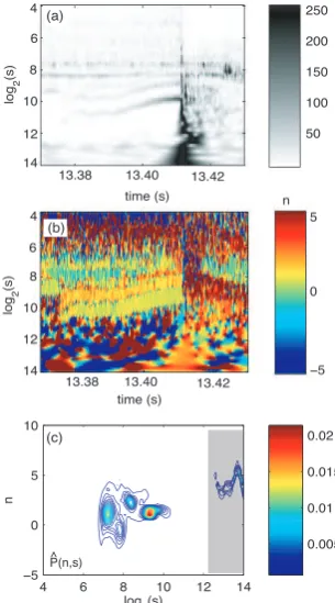
z=1.013 m over the equatorial plane, and toroidally sep-arated. Two coils are 10.17 degrees apart, allowing the measurement of toroidal mode numbers up to 15, the sec-ond pair has mutual separation of 5.63 degrees and allows the measurement of toroidal mode numbers up to 30. Figure 2 shows the wavelet scalogram (the equivalent of spectrogram with frequencies replaced by scales) com-puted from (4) in the case of pulse #42976, in a time win-dow centered on the ELM. The ELM precursor, an ex-ternal kink mode [5], is indicated in the wavelet scalo-gram as the coherent mode that starts from t ∼ 13.37 s and whose frequency increases with time. The ELM is seen in the wavelet scalogram as a structure that ex-tends from low to high frequencies. The distortion in the spectrum at large scales, typical for continuous wavelet transforms [12], mask low frequency spectral features; we therefore discard spectral components at scales larger than log2(s)=12, corresponding to frequencies below 1 kHz, in
our discussion. The toroidal mode number can be inferred
lo g
2 (s)
n
4 6 8 10 12 14
−5 0 5 10
0.005 0.01 0.015 0.02
lo
g 2
(s)
lo
g 2
(s)
4
4
6 6
8 8
10
10
12 12
14
14 13.38 13.38
13.40
13.40 13.42
13.42 time (s)
time (s)
−5 0 5 50 250
200
150
100
n
(c) (b) (a)
P(n,s) ^
Fig. 2 JPN 42976. (a) Normalized wavelet coefficients. (b)
toroidal mode number. (c) Normalized spectrum ˆP(n,s),
computed from the wavelet coefficients in the time
win-dow between 13.37 s and 13.41 s.
from the phase shift between two Mirnov coils divided by their toroidal separation as:
n= 1 Δφarg[W
∗
m(φ1,s)Wm(φ2,s)] (6)
and it is shown in Fig. 2(b). While the toroidal mode number of the precursor is easily identified in the phase spectrogram, the toroidal mode number get confused in the plot when approaching the ELM and it is difficult to
drive any conclusion. The phase shift undertakes jumps of 2πright before the ELM crash and coherent modes spread
in toroidal mode number. In order to better visualize the range of toroidal mode numbers involved during the phases that immediately precede the ELM, and during the ELM burst itself, we have applied a statistical analysis based on a two-point correlation technique [9]. After having computed the wavelet coefficients from (4), we have
con-structed the mode number and frequency spectrumP(n,s) as follows:
P(n,s)= 1 N
N
�
j=1
IΔ[nj−n¯]P(s) (7)
whereP(s) = 0.5×[P1(s)+P2(s)] is the average of the
power spectra measured at positions φ1 andφ2,
[image:4.595.368.521.85.360.2]minimal differences in the final results. The toroidal mode
numbernjis computed from the wavelet coefficients, using
Eq. (6), with the index jrunning over time. The indicator functionIΔ, the discrete equivalent of the delta function, is
defined as:
IΔ[nj−n¯]=
�
1 ¯n−Δ≤nj<n¯+ Δ
0 elsewhere (8)
Computing (7) is equivalent to constructing a histogram. For each time step tj = jts, the value of the toroidal
mode number nj is compared with the reference values
of ¯n = [−30,30]. The bin width has been chosen equal to Δ = 0.5 cm−1, in order to minimize the variance of
the power spectrum estimate. The outcome is a robust estimate of the frequency- wavenumber power spectrum [16]. Following [9] we define the conditional spectrum,
P(n|s)=P(n,s)��sP(n,s)�−1, which can be interpreted as
the probability that a mode measured at frequencys−1has
toroidal mode number n. Figure 2(c) shows the normal-ized spectrum ˆP(n,s) = P(n,s)[�s,nP(n,s)]−1 computed
in the time window between 13.37 s and 13.41 s. Dur-ing this phase the dominant contribution to the total power spectrum is given by the ELM precursor and its harmonics, represented in the plot as ‘spots’ with toroidal mode num-ber n = 1,2,3 and log2(s) between 6 and 10. As shown
in Fig. 2(a), the measured frequency of the precursor in-creases (i.e. the wavelet scale dein-creases), as well as the amplitude of the fundamental harmonics. The contribu-tion to the total power spectrum is therefore larger in the latest time phase, approaching the burst. Figure 3 shows
P(n,s) and P(n|s) computed in two time windows. The first windowt = [12.4110,12.4112] s corresponds to the 200 μs that precede the ELM, while the second window,
t =[12.4112,12.4116] s covers the ELM burst, which co-incides with the phase when the Dα emission rapidly
in-creases. Since the phase undertakes jumps of 2πin these windows, we have computed the toroidal mode number from the pair of Mirnov coils with the smaller toroidal separation, Δφ ∼ 5.63 degrees. The results of the
anal-ysis coincide with the results obtained from the pair with larger toroidal separation in frequency ranges where the phase variations are smooth, but are less affected by phase
jumps during the ELM crash. From a comparison be-tween Fig. 2(c) and Fig. 3(a) we can see that the toroidal mode number structure changes during the phases that im-mediately precede the ELM. During the 200-300 μ that
precede the burst, the maximum contribution to the total power spectrum comes from spectral components with low toroidal mode number,n=1,2 and frequencies lower than that of the precursor [log2(s) > 10]. These components also have a smooth variation in the toroidal mode number, which tends to increase in absolute value, as it is made more evident in the conditional spectrum, Fig. 3(b). A jump in the phase is measured at log2(s) ∼ 12, although we remind that spectral components with scale larger than this value are not discussed herein.
As shown in Fig. 3(b), spectral components with loga-rithmic scale between 6 and 7 have toroidal mode num-bers regularly distributed between±10, while at smaller scales, namely frequencies larger 100 kHz, the toroidal mode number is spread between±30, with no clear trend. In this frequency range the power spectral density is low and mode phase have poor correlation. During the ELM crash, the toroidal mode number measured in the range of scales where the precursor is detected, with [log2(s)=8 to
10, evolves towards even larger values, up to 25. The spec-trum at lower frequencies stays almost unaffected, with
toroidal mode numbers low in value, while the spectrum at larger frequencies develops a more clear structure, with definite frequencies associated with definite toroidal mode numbers. We cannot exclude that the toroidal mode num-ber in this range of frequencies may be even larger than those measured here and that these apparent trends at high frequency are partly due to an aliasing effect. The
mea-sured range ofn values suggest that the ELM instability has a ballooning character. The evolution of toroidal mode number towards larger values has been predicted by ideal MHD theory [17], although the simulations in that case were done assuming that the ELM precursor was a balloon-ing instability withn∼5, while in this case the precursor is an external kink mode. Evidence for increasing in the toroidal mode number were also derived from target load pattern on ASDEX-U where, in the start phase of the ELM collapse isn ∼3−5, evolving to values ofn ∼ 12−14 during the ELM power deposition maximum [18].
4. Conclusions
An approach is suggested for determining toroidal mode numbers of ELMs, suitable for the short time scales involved in the ELM dynamics. The technique, commonly used to recover the dispersion relation of waves in plasmas [16], consists of a wavelet analysis, which provides good resolution in time, supplemented by a two-point correla-tion technique, which provides a robust statistical recon-struction of toroidal mode numbers involved in an ELM event. Using a wavelet-based two-point correlation, the coherent part of the ELM spectrum is enhanced, while the incoherent part is averaged out giving negligible contribu-tion to the total spectrum. The applicacontribu-tion of the method to H-mode plasma discharges with type-I ELMs on JET indicates that spectra with statistical significance can be obtained over time windows of 50μs length. It is found that the toroidal mode number of a type-I giant ELM, ob-served in a D-T plasma discharge starts from low toroidal mode numbers, consistently with the toroidal mode num-ber of the precursor, an external kink mode withn = 1
[5]. The toroidal mode number increases approaching the ELM and a broad range of values, from 1 to 30 are mea-sured during the burst, indicating that the ELM consists of the superposition of many modes. Preliminary analysis over H-mode type-I ELMs confirm these results, indicating
402
n
P(n,s) (a)
4 6 8 10 12 14
−30 −20 −10 0 10 20 30
0.01 0.02 0.03 0.04
log 2 (s )
n
(c)
4 6 8 10 12 14
−30 −20 −10 0 10 20 30
0.01 0.02 0.03 0.04
n
P(n|s) (b)
4 6 8 10 12 14
−30 −20 −10 0 10 20 30
0.2 0.4 0.6 0.8
log 2 (s )
n
P(n|s) (d)
4 6 8 10 12 14
−30 −20 −10 0 10 20 30
0.2 0.4 0.6 0.8 ^
P(n,s) ^
Fig. 3 (a) Normalized spectrumP(n,s), computed from the wavelet coefficients in the time windowt=[12.4110,12.4112] s, before the
ELM crash. (b) Conditional spectrum, in the same time window. (c)-(d) Same as (a) and (b) but during the ELM, between 12.4112 s and 12.4116 s. Shaded areas indicate the range of scales that is discarded in the discussion.
that the toroidal mode number of an ELM increases imme-diately before the burst, although the maximum value may vary depending on the background plasma. Deeper analy-sis over a set of JET discharges is ongoing, including the cases of ELMs triggered by pellets and ELMs mitigated by Error Field Correction Coils.
This work has been conducted under the European Fu-sion Development Agreement. The views and opinions ex-pressed herein do not necessarily reflect those of the Euro-pean Commission. F M. Poli is funded by the UK EPSRC.
[1] Perez C. P, Koslowski H. R, Huysmans G. T. A,et al, Nucl. Fusion,44, 609 (2004).
[2] Zohm M, Plasma Phys. Control. Fusion,38, 105 (1996). [3] Kamiya K, Asakura N, Boedo J, et. al, Plasma Phys.
Con-trol. Fusion,49, S43 (2007).
[4] Connor J. W, Plasma Phys. Control. Fusion,40, 191 (1998).
Ibid,40, 531 (1998)
[5] G T A Huysmans, S E Sharapov, A B Mikhailovskii and W Kerner, Phys. Plasmas8, 4292 (2001).
[6] H.R. Wilson and S.C. Cowley, Phys. Rev. Lett.92, 175006 (2004).
[7] T Kass, S G¨unteret al, Nucl. Fusion,38111 (1998). [8] F M Poli, S E Sharapov, S C Chapmanet al, Plasma Phys.
Control. Fusion,50095009 (2008).
[9] J. M. Beall, C. Kim, and E. J. Powers, J. Appl. Phys.53, 3933 (1982).
[10] M Keilhacker, Nucl. Fusion39, 209 (1999).
[11] R. F. Heeter, A. F. Fasoli, S. Ali-Arshad, and J. M. Moret, Rev. Sci. Instrum.,714092 (2000)
[12] S Mallat, A wavelet tour of signal processing, chapter 4. Academic Press, Cambridge, (2001).
[13] A I Eriksson, Spectral analysis, in Analysis Methods for Multi-Spacecraft Data, ISSI Scientific Report, G Paschmann and P W Daly (Eds), ISSI, Bern (1998)
[14] C Torrence and G P Compo, Bulletin of the American Me-teorological Society,7961 (1998)
[15] R. Koslowski et al., Nucl. Fusion45, 201 (2005).
[16] T. Dudok de Wit, V V Krasnosel’skikh,et al, Geoph. Res. Lett. 22, 2653, 1995.
[17] G T Huysmanset al, Proceedings of the 35thEPS Plasma Physics Conference, Hersonissos, Crete, Greece, (2008). [18] T Eich, A Herrmannm J Neuhauseret al, Plasma Phys.
[image:6.595.109.488.72.288.2]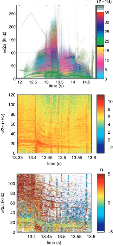
![Fig. 3(a) Normalized spectrum P(n, s), computed from the wavelet coefficients in the time window t = [12.4110, 12.4112] s, before theELM crash](https://thumb-us.123doks.com/thumbv2/123dok_us/9719320.472906/6.595.109.488.72.288/normalized-spectrum-computed-wavelet-coecients-window-theelm-crash.webp)
