Quantifying the impacts of climate driven flood risk changes and risk perception biases on coastal urban property values ; A case study for the North Carolina coastal zone

(1)

Quantifying the impacts of climate-driven

flood risk changes and risk perception

biases on coastal urban property values

-A case study for the North Carolina coastal

zone-JOHAN DE WAARD

May 11, 2015

(2)

(3)

i Title: Quantifying the impacts of

climate-driven flood risk changes and risk perception biases on coastal urban property values

Subtitle: A case study for the North Carolina coastal zone

Thesis for the degree of Master of Science in Civil Engineering and Management

Author: Johan de Waard

Institute: University of Twente

Department: Water Engineering and Management

Supervisors: Prof. dr. S.J.M.H. Hulscher

Department of Water Engineering and Management

dr. T. Filatova

Centre for Studies of Technology and Sustainable Development (CTSM)

dr. ir. E.M. Horstman

Department of Water Engineering and Management

Date: May 11, 2015

(4)

(5)

iii

Summary

Between 1991 and 2010, hurricanes and tropical storms were the biggest cause of property losses, causing 44% of all disaster related property destruction in the U.S. The projected growth in population of coastal counties, with the accompanying rise in coastal asset value, in combination with the impacts of the expected ongoing climate change poses an ever growing financial liability to the U.S. taxpayer and coastal resident. Since housing is a major source of collateral for the financial system, being able to simulate property values may help reveal the true risk of future climate change to financial institutions. However, the market value of these houses is influenced by the risk perception bias of buyers who operate in the market. This research focusses on these subjects affecting coastal urban property values and are reflected in the research objective:

“To quantify the impacts of climate change, and the effect of the associated flood risks and risk perception bias on coastal urban property values at the North Carolina coastal zone.”

First, the impacts of climate change on Beaufort (Carteret County, North Carolina, U.S.) for the year 2050 is downscaled from the global climate change scenarios. Carteret County is one of the counties most often hit by a hurricane and as it is situated on the coastal plain, regional sea level rise and changing hurricane frequencies will be the focus of the climate change impacts. The regional sea level rise for the year 2050 is less than 30 cm, this is too small to be used during this study and is therefore omitted. For Carteret County the dominant source of flooding are wind driven storm surges associated with hurricanes. Under climate change conditions the current 100 year storm will have a return period of 61 years by 2050 and the current 500 year storm will be more than twice as likely to occur in 2050 with a decreased return period of 231 years.

Second, divided into three subjects, risk will be explored by taking a look at objective risk, subjective risk, and the risk perception bias procedure. The objective risk is either the current flood risk probability, as determined by the Federal Emergency Management Agency, or the hurricane return period under climate change. Housing market actors will assess objective flood risk on the basis of probability and severity of damage, this is the subjective risk, and will be biased by myopia and amnesia. The risk perception bias procedure is started by a flood event, over a period of 5 years the bias declines logarithmically from its maximum to its minimum level.

(6)

(7)

v

Preface

In November 2014 I started with the final leg of my study Civil Engineering at the University of Twente. Today six months later, I am proud to present the findings of my research. The goal of this research has been to quantify the impacts of climate change and risk perception bias on coastal urban property values, however, this study has also provided me with the opportunity to improve my modelling and analytical skills and my academic writing.

I would like to thank my supervisors, Tatiana, Erik, and Suzanne, for all their help in bringing my thesis to a successful end and for all the times is was able to barge into your offices unannounced with yet another question.

Next I would like to thank my sister Eveline, who always told me I could do it even when I didn’t think I could. To my girlfriend Sofieke, who kept me going during a very difficult year even when I thought the situation was hopeless.

A special thank you is reserved for my parents, Peter and Petra, without whom I never would have been able to spend all these wonderful years as a student in Enschede. Papa en mama, bedankt voor alles.

(8)

(9)

1

List of acronyms

ABM Agent-based modeling AR4 Fourth Assessment Report AR5 Fifth Assessment Report

CMIP3 Coupled Model Intercomparison Project 3

ENSO El Niño-Southern Oscillation

GHG Green House Gases

GIA Glacial Isostatic Adjustment

GMSL Global Mean Sea Level

IPCC Intergovernmental Panel on Climate Change

NAO The North Atlantic Oscillation

NOAA National Oceanic and Atmospheric Administration

PDO Pacific Decadal Oscillation

RCP Representative Concentration Pathways RF Radiative Forcing

RHEA Risks and Hedonics in Empirical Agent-based land market model

RSL Relative Sea level

SRES Special Report on Emission Scenarios

TAR Third Assessment Report WGI Working group 1

EU Expected Utility

(12)

4

1. Introduction

In this first chapter the background for this research will be presented. The research objective and the research objectives that are addressed in this thesis will be introduced. The methodology and scope are discussed before ending the introduction with the research strategy and thesis outline presenting a guide to the coming chapters.

Background

1.1.

Flooding is the most common natural disaster in the United States. Between 1991 and 2010, hurricanes and tropical storms were the biggest cause of property losses among all natural catastrophes, causing 44 percent of all disaster related property destruction in the U.S. (Polefka, 2013). With the global climate changing and its projection to continue changing over this century (Melillo, Richmond, & Yohe, 2014) coastal systems and low-lying areas will increasingly experience the adverse effects of climate change. As of 2010 39% of the U.S. population lives in counties with a coastline. Between the period of 1970-2010 these coastal shoreline counties have seen a large increase in population and are projected to grow even further (Crosset, Ache, Pacheco, & Haber, 2013). The projected growth in population of coastal counties, with the accompanying rise in coastal asset value, in combination with the impacts of the expected ongoing climate change poses an ever growing financial liability to the U.S. taxpayer and coastal resident.

Since housing is a major source of collateral for the financial system, being able to simulate property values may help reveal the true risk of future climate change to financial institutions. The worldwide economic crisis starting with the U.S. sub-prime mortgage crisis has revealed how vulnerable the world’s financial system is to changes in property values. An important implication of growing flood risks is in the destabilizing effect that the resulting unanticipated house price declines can have (Pryce, Chen, & Galster, 2011).

It is important to keep in mind that the market value of houses vulnerable to flooding forms the basis of estimating direct flood damage in residential areas. However, the market value of these houses is influenced by the risk perception bias of buyers who operate in the market. A price discount effect exists which changes with time, this discount effect is connected with the risk perception bias of buyers, it grows after a disaster and vanishes shortly after. The dynamics of the risk perception bias requires an adaptive model such as the RHEA model. In this respect a purely hedonic model would not have been an option, since hedonics use a snapshot of the market in time. A statistical spatial model would be equally unsuitable as it wouldn’t allow for changes in individual demand due to dynamic risk perceptions reflected in housing prices.

Research objective and research questions

1.2.

(13)

5

“To quantify the impacts of climate change, and the effect of the associated flood risks and risk perception bias on coastal urban property values at the North Carolina coastal zone.”

Using global and local climate change scenarios for the U.S. Atlantic coast, the influence of climate change on coastal zones will be determined for the main climate impacts: relative sea level rise and extreme sea level events (Field et al., 2014). The impacts of relative sea level rise and extreme sea level events on the coastal zone will be used to determine changing flood risks and perceived risks for coastal properties and its consequences for coastal property values. In order to help achieve the research objective, the following research questions have been formulated:

1. To what extent will future climate change affect flood risks of the North Carolina coastal zone?

a. What climate change scenarios are expected for the North Carolina coastal zone? b. What are the effects of climate change on submergence for the North Carolina

coastal zone?

c. What are the effects of climate change on coastal flooding for the North Carolina coastal zone?

2. How can (changes to) future flood risks and risk perception bias be simulated for the North Carolina coastal zone under variable climate change scenarios?

a. How are the effects of flood risks on property values to be simulated with the RHEA model?

b. How is risk perception bias to be incorporated into the RHEA model?

3. What is the impact of coastal flood risk changes and risk perception bias on coastal property values at the North Carolina coastal zone?

a. Which scenarios should be considered to determine the impact of coastal flood risk changes and risk perception bias on coastal property values at the North Carolina coastal zone?

b. How is the total market value of coastal properties affected under the different scenarios?

c. How is the average market value of coastal properties affected under the different scenarios?

d. How is the number of trades of coastal properties affected under the different scenarios?

Methodology

1.3.

This section describes the methodology used in this research, to allow the research objective to be achieved. The research questions show us that this research will comprise three parts: (i)climate change and the consequent flood risk changes; (ii) the modelling of future coastal property values when exposed to flood risk and the way to include risk perception in this modelling; and (iii) a study of the impacts of climate change and risk perception on future coastal property values.

(14)

6

Downscaling the global climate change scenarios allows the relevant climate impacts to be identified as well as the magnitude of these climate impacts.

Part 2 starts by properly identifying the kinds of risk relevant to this research, to be able to properly assess the impacts of risk perception bias. Once identified were the risk perception bias comes from, how this functions, and how it should operate within the market a procedure can be written to incorporate it into the existing RHEA model.

The final part will combine climate change and risk perception bias in order to reach the research objective. In order to properly analyze the scenarios, the results will be indexed. The starting values of each scenario will be the base index and therefore receive the index value 100, this allows to quickly assess the results.

Scope

1.4.

The research questions introduced above will be addressed through a case-study for the North-Carolina coast. The study area chosen for this study is narrowed down to the town of Beaufort located in Carteret County, North Carolina in the U.S. Beaufort has been used as study area before in a number of different studies e.g. (Bin, Kruse, & Landry, 2008; Bin, Poulter, Dumas, & Whitehead, 2011; Filatova & Bin, 2013; Filatova, 2014), this means that relevant data for Beaufort is available as well as a valid representation within the RHEA model. This chapter contains a brief description of the study area.

1.4.1. Beaufort, Carteret County, North Carolina

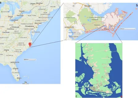
The study area is located on the eastern seaboard of the United States, in Beaufort, Carteret County, North Carolina (Figure 1). North Carolina’s coastal plain covers almost half of North Carolina (Wikipedia, 2015), with 5000 km2 of the land area below 1 m elevation this part of North Carolina is very vulnerable to sea level rise (Bin et al., 2011).

Carteret county (Figure 1b) is one of the counties most affected by hurricanes, 22 hurricane strikes have been reported to hit Carteret county between 1900 and 2010 (NOAA National Hurricane Center, 2014). On the eastern U.S. seaboard only three counties have had more hurricane hits. Two of these counties are located on the most southern tip of Florida and the third one is Dare county which is situated to the north-west of Carteret county.

(15)

[image:15.595.72.520.74.392.2]

7

Figure 1: Location of Beaufort in the continental United States and overview of the study area (c). Top images (a and b) from (Google, 2015), bottom image from (Filatova, 2014).

1.4.2. Coastal characteristics

(16)

8

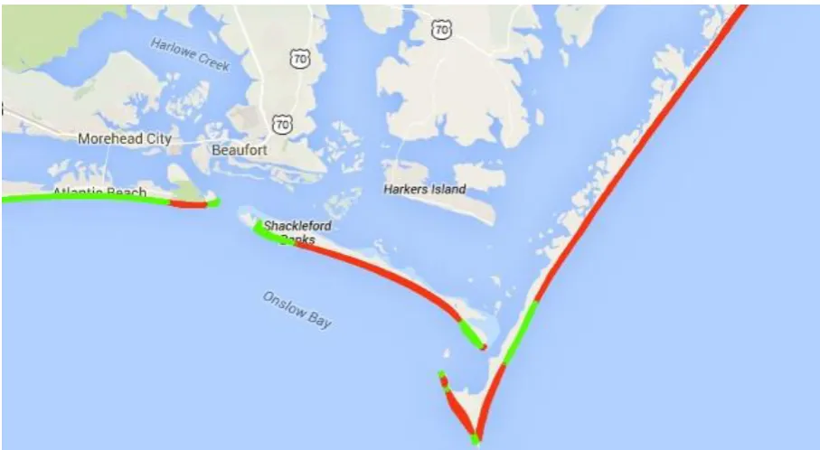
Figure 2: Erosion and accretion of the barrier islands visualized, red shows erosion and green shows accretion (N.C. Division of Coastal Management, 2014).

Research strategy and thesis outline

1.5.

To answer the research questions and to achieve the research objective put forward in the previous section, the strategy described below is used.

Chapter 1.4 introduced the scope. In this chapter we take a look at Beaufort, North Carolina, both geographically and demographically. By studying Beaufort we can determine which climate impacts (increasing flood damage, dry-land loss due to submergence and/or erosion(Field et al., 2014)) are relevant physical impacts of future climate change, as is put forward in the central research question. Chapter 2 is devoted to the RHEA model. In this chapter we will take a look at agent based modeling in general, discuss the RHEA model, look into the input needed to run the model, and review the sensitivity of the RHEA model to its input parameters.

The objective behind research question 1a is to find the proper information on climate change scenarios to be used in this research. Chapter 3 aims to achieve this objective by making use of existing climate studies performed on both a global scale as well as a regional scale. The studies done by the Intergovernmental Panel on Climate Change and local subsidiaries will provide the relevant information on the expected global and local climate change.

[image:16.595.70.524.72.321.2]

(17)

9

The objective behind research question 2 is to define a way to simulate flood risk under climate change conditions as well as risk perception bias, both within the RHEA model. Chapter 4 seeks to achieve this objective and provides methods to quantify the levels of flood risk, both objective as well as subjective, for Beaufort and its residents.

The answers to the final research question will be able to form a bridge between climate change and risk perception bias in chapter 5. In response to research question 3a, this chapter will first define the scenarios to be used in the simulations with the RHEA model. The results from these simulations will be compared in order to obtain insights regarding research question 3b.

(18)

10

2. Model description

This chapter explores the model which lies at the basis of this research. First we take a look at agent-based models in general. Then the RHEA model is introduced, including the input required to run the model.

Agent-based models

2.1.

Agent-based modeling (ABM), also known as individual-based modeling, is the modeling of phenomena as dynamical systems of interacting agents (Castiglione, 2006). In ABM, a system is modeled as a collection of autonomous decision-making entities called agents. Each agent individually assesses its situation and makes decisions based on a set of rules. This makes it possible to study the combined effect of individual decisions on a systems level (Bonabeau, 2002). ABM allows one to simulate the individual actions of diverse agents, measuring the resulting system behavior and outcomes over time (Crooks, Castle, & Batty, 2008).

Compared to other modelling techniques the benefits of ABM can be made in three statements: (i) ABM captures emergent phenomena; (ii) ABM provides a natural description of a system; (iii) ABM is flexible, it is easy to add more agents and it provides a natural framework for tuning the complexity of the agents (e.g. behaviour, degree of rationality, ability to learn and evolve and rules of interaction) (Bonabeau, 2002).

RHEA model

2.2.

The Risks and Hedonics in Empirical Agent-based land market (RHEA) model was introduced by Filatova (2014). The RHEA model captures natural hazard risks and environmental amenities through hedonic analysis and allows for empirical agent-based land market modeling. In this section a description of the most relevant aspects of the model will be given. For additional information on the model, the reader is directed to the paper by Filatova (2014) on the RHEA model.

(19)

11

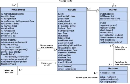
Figure 3: Unified Modeling Language class diagram of the housing market: agents, their properties and functions.

(Filatova, 2014)

The trading of residential properties and the allocation of households in a town is the main process in the ABM. Each time step the trade process consists of several phases: listing of vacant spatial goods in a market by sellers; search for the best location under budget constraint by buyers; formation and submission of bids by buyers to sellers; evaluation of received bids by sellers; price negotiation, transaction and registration of trade; and finally updating of market expectations by realtors (real estate agents). The sequence of events in one time step is presented in Figure 4.

[image:19.595.70.524.75.369.2]

(20)

[image:20.595.78.508.77.662.2]

12

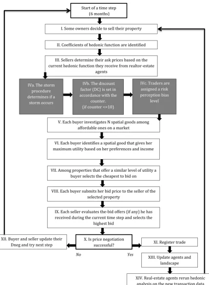
Figure 4: Dynamics of the trade process: a sequence of actions, which agents perform within 1 time step of the bilateral agent-based housing market with expectations formation (Updated from Filatova, 2014). Boxes IVa,b,c show the procedures which have been added during the course of this research, the NetLogo code for these procedures can be found in appendix D2.

When choosing a location in a coastal town with designated flood zones, a household operates under the conditions of uncertainty due to the flood risk at the location of the property. Since a buyer

Start of a time step (6 months)

I. Some owners decide to sell their property

II. Coefficients of hedonic function are identified

III. Sellers determine their ask prices based on the current hedonic function they receive from realtor-estate

agents

V. Each buyer investigates N spatial goods among affordable ones on a market

VI. Each buyer identifies a spatial good that gives her maximum utility based on her preferences and income

VII. Among properties that offer a similar level of utility a buyer selects the cheapest to bid on

VIII. Each buyer submits her bid price to the seller of the selected property

IX. Each seller evaluates the-bid offers (if any) he has received during the current time step and selects the

highest bid

X. Is price negotiation

successful? XI. Register trade

XII. Buyer and seller update their Dneg and try next step

XIII. Update agents and landscape

XIV. Real-estate agents rerun hedonic analysis on the new transaction data

No Yes

IVa. The storm procedure determines if a

storm occurs

IVb. The discount factor (DC) is set in accordance with the

counter. (if counter <=10)

IVc. Traders are assigned a risk perception bias

(21)

13

searches for a property that will maximize its utility, the buyer will now aim to maximize its expected utility (EU). Utility is defined as the enjoyment or satisfaction people receive from consuming goods and services (Hubbard, Garnett, Lewis, & O’Brien, 2014). When a buyer is trying to maximize utility, he is looking for the property that will give him the most satisfaction considering his preferences and income.

𝐸𝑈 = 𝑃_𝑖𝑈_𝐹+ (1 − 𝑃_𝑖)𝑈𝑁𝐹 [1]

Wherein UF is the utility in case of a flood, UNF the utility in case of no flood and Pi is the subjective

perception of risk the buyer has. Equations [2] and [3] show the respective formulas for UF and UNF:

𝑈𝐹 = 𝑠𝛼(𝑌 − 𝑇(𝐷) − 𝑘𝐻𝐻𝑎𝑠𝑘− 𝐿 − 𝐼𝑃 + 𝐼𝐶)1−𝛼𝐴𝛾 [2]

𝑈_𝑁𝐹 = 𝑠𝛼_{(𝑌 − 𝑇(𝐷) − 𝑘}

𝐻𝐻𝑎𝑠𝑘− 𝐼𝑃)1−𝛼𝐴𝛾 [3]

Calculating the household’s utility depends on housing goods (s) which are affordable for the buyer in their budget (Y) net of transport costs (T(D)). Preferences for housing goods and amenities are represented by α and γ, respectively. (L) represents the damage in case of a flood, (IP) the insurance premium and, (IC) the insurance coverage in case of a disaster. The buyers search for the property that provides the highest utility to them. Once a buyer has located the property that yields the highest utility, a bid price is offered to the seller (box VII, Figure 4) and price negotiations will start, Figure 33 in appendix C1 shows the price negotiation process (Filatova, 2014).

Model input

2.3.

The RHEA model requires a number of different input parameters to be able to run. Spatial data is extracted from GIS data sets defining the locations of residential housing, coastal amenities, distances to the central business district, and others. Realtor-agents in the model use the empirical hedonic function developed by Bin et al. (2008), which is based on the real estate transactions from 2000 to 2004. To run the hedonic function, structural characteristics of the property, such as total square footage and the number of bathrooms, are required along with data on households incomes and preferences. Flood zones and the associated flood probability of 1:100 and 1:500 are represented as well. The remaining input parameters, their abbreviations and a short description of what they do can be found in Table 13 in appendix C2.

Changes in the RHEA model

2.4.

(22)

14

3. Climate change and its impacts

In this chapter we will discuss climate change and the relevant impacts climate change have on the study area. We start by examining the latest climate change scenarios developed by the Intergovernmental Panel on Climate Change. Both the global mean temperature change and the Eastern North American mean temperature change are discussed. The regional climate change models examine the Eastern North American mean temperature change.

In chapter 1.4 we learned that Carteret County is one of the counties most often hit by a hurricane and as it is situated on the coastal plain, sea level rise is a serious threat as well. Beaufort however, is not affected by erosion as the barrier islands protect it. This chapter will conclude with investigating how local sea level rise and hurricane frequencies change under climate change scenarios.

Global climate change

3.1.

Late September 2013 the results from Working Group I (WGI) of the Intergovernmental Panel on Climate Change for the Fifth Assessment Report (AR5) were released. One of the most notable changes in the AR5 are the scenarios for future emissions of greenhouse gases. The Fourth Assessment report (AR4) made use of the socio-economic driven scenarios developed by the IPCC (2000). These scenarios resulted from specific socio-economic scenarios from storylines including future demographic and economic development, regionalization, energy production and use, technology, agriculture, forestry and land use (Cubasch et al., 2013). Even though the scenarios from the Special Report on Emissions Scenarios have been productive (Moss et al., 2010), new scenarios were needed. A decade worth of new data, economic, environmental, and new technologies had to be incorporated in these new scenarios.

For AR5, multiple Representative Concentration Pathway (RCP) scenarios were developed. These scenarios specify concentrations and corresponding emissions, but are not directly based on socio-economic storylines as were the scenarios used in AR4. However, these RCP scenarios can potentially be realized by more than one socio-economic scenario (Collins et al., 2013). A set of four RCP scenarios has been developed and is used as a basis for long-term and near-term modeling experiments (Van Vuuren et al., 2011), the four RCP scenarios are further explained in appendix A1. Table 1 shows the predicted global temperature change for the years 2050 and 2100 under the four RCP scenarios.

Table 1: The four RCP scenarios and predicted global temperature increase by 2050 and 2100 (data from van Oldenborgh et al., 2013). A more extensive look into global temperature change for the RCP scenarios can be found in appendix A2.

Scenario Temperature increase by 2050

Temperature increase by 2100

RCP 2.6 1.00 °C 0.96 °C

RCP 4.5 1.32 °C 1.89 °C

RCP 6.0 1.16 °C 2.43 °C

(23)

15

Projections based on the SRES A1B scenario show that it is likely that the global frequency of tropical cyclones will either decrease or remain as they are now. The mean intensity, which is measured by the maximum wind speed, will increase between +2 and +11 percent. Associated rainfall rates can increase by as much as 20 percent within a radius of 100 km of the cyclone center.

Regional climate change

3.2.

“Regional climates are the complex outcome of local physical processes and the non-local responses to large-scale phenomena such as the El Niño-Southern Oscillation (ENSO) and other dominant modes of climate variability” (Christensen et al., 2013).

3.2.1. Regional temperature

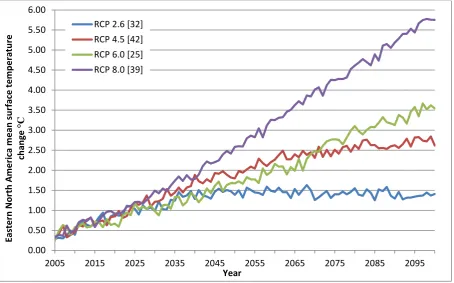
The North American climate is affected by 7 major climate phenomena, these climate phenomena influence aspects of the North American climate such as temperature and precipitation (Christensen et al., 2013). What these climate phenomena are and what their effects on the climate projections are, is not relevant. However, what is relevant is that these climate phenomena cause the expected increase in surface temperature change for the 21st Century for Eastern North America to deviate from the global mean surface temperature change. Figure 5 shows the multi-model mean surface temperature change for Eastern North America, where the study area is located.

The patterns observed in Figure 5, where RCP 2.6 shows stabilization in global warming, RCP 4.5 shows higher warming than RCP 6.0 until 2065 and RCP 8.5 shows by far the highest warming for the year 2100 resembles the patterns of warming of the global multi model mean surface temperature change (Figure 31, appendix A2).

Figure 5: Multi model mean of Eastern North America mean surface temperature change for the four RCP scenarios relative to 1986-2005. Number of models per scenario can be found in the brackets (data fromvan Oldenborgh et al., 2013). 0.00 0.50 1.00 1.50 2.00 2.50 3.00 3.50 4.00 4.50 5.00 5.50 6.00

2005 2015 2025 2035 2045 2055 2065 2075 2085 2095

Easte rn N o rth A m e ri ca m e an su rface t e m p e ratu re ch an ge °C Year RCP 2.6 [32]

[image:23.595.72.527.442.725.2]

(24)

16

3.2.2. Cyclones

Cyclones are also named typhoons or hurricanes. The term typhoon is used for cyclones occurring in the Pacific Ocean and the word hurricane is used for cyclones in the Atlantic Ocean. Two different types of cyclones can be distinguished: the tropical cyclone and the extra-tropical cyclone. A tropical cyclone is a non-frontal synoptic scale low-pressure system over tropical or sub-tropical waters with organized convection (i.e. thunderstorm activity) and definite cyclonic surface wind circulation (Landsea, 2011). An extra-tropical cyclone ‘is a storm system that primarily gets its energy from the horizontal temperature contrasts that exist in the atmosphere. Extra-tropical cyclones are low pressure systems with associated cold fronts, warm fronts, and occluded fronts (Goldenberg, 2004). Structurally, tropical cyclones have their strongest winds near the earth's surface, while extra-tropical cyclones have their strongest winds near the tropopause - about 12 km up. These differences are due to the tropical cyclone being "warm-core" in the troposphere (below the tropopause) and the extra-tropical cyclone being "warm-core" in the stratosphere (above the tropopause) and "cold-core" in the troposphere. "Warm-core" refers to being relatively warmer than the environment at the same pressure surface (Goldenberg, 2004).

3.2.2.1. Tropical cyclones

Assessing changes in regional tropical cyclone frequency is still limited because confidence in projections critically depend on the performance of control simulations, and current climate models still fail to simulate observed temporal and spatial variations in tropical cyclone frequency (Christensen et al., 2013). A downscaling study done by Bender et al. (2010) suggests that the predicted increases in the frequency of the strongest Atlantic storms may not emerge as a statistically significant signal until the latter half of the 21st century.

3.2.2.2. Extra-tropical cyclones

Climate change studies have shown that precipitation is projected to increase in extra-tropical cyclones despite there being no increase in wind speed or intensity of extra-tropical cyclones. (Christensen et al., 2013)

Sea level rise

3.3.

Sea level rise over the coming centuries is amongst the potentially most serious climate change related impacts (Jevrejeva, Moore, & Grinsted, 2012; Vermeer & Rahmstorf, 2009). The economic costs and the social consequences related to coastal flooding and forced migration will probably be one of the most important impacts of global warming (Sugiyama, Nicholls, & Vafeidis, 2008). Paleolithic sea level records from the warm periods which occurred during the last 3 million years have indicated that the global mean sea level (GMSL) exceeded 5 meters above present GMSL records. However, the global mean temperature during these warm periods was only up to 2°C warmer than pre-industrial levels (Church et al., 2013). To put this into context, the projected global mean temperature change under RCP 6.0 by the year 2100 is 2°C and the 5% confidence interval for RCP 8.5 for the year 2100 is already well beyond the 2°C mark (IPCC, 2013).

3.3.1. Global sea level rise

(25)

17

subsequent runoff to the ocean) also affects the mean sea level (Stocker et al., 2013). Since the late 1800s, tide gauges throughout the world have shown that global sea level has risen by about 20 centimeters on average. This recent rise is much greater than at any time in at least the past 2000 years. Since 1992, the rate of global mean sea level rise measured by satellites has been roughly twice the rate observed over the last century (Walsh et al., 2014). The rate of GMSL rise during the 21st century will most likely exceed the rate of GMSL rise observed during the last 40 years for all RCP scenarios. This is due to increases in ocean warming and loss of mass from glaciers and ice sheets. Table 2: Global mean sea level rise (m) with respect to 1986–2005 at 1 January on the years indicated. Values shown as median [likely range]. (IPCC, 2013)

Year RCP 2.6 RCP 4.5 RCP 6.0 RCP 8.5

2007 0.03 [0.02 to 0.04] 0.03 [0.02 to 0.04] 0.03 [0.02 to 0.04] 0.03 [0.02 to 0.04] 2010 0.04 [0.03 to 0.05] 0.04 [0.03 to 0.05] 0.04 [0.03 to 0.05] 0.04 [0.03 to 0.05] 2020 0.08 [0.06 to 0.10] 0.08 [0.06 to 0.10] 0.08 [0.06 to 0.10] 0.08 [0.06 to 0.11] 2030 0.13 [0.09 to 0.16] 0.13 [0.09 to 0.16] 0.12 [0.09 to 0.16] 0.13 [0.10 to 0.17] 2040 0.17 [0.13 to 0.22] 0.17 [0.13 to 0.22] 0.17 [0.12 to 0.21] 0.19 [0.14 to 0.24] 2050 0.22 [0.16 to 0.28] 0.23 [0.17 to 0.29] 0.22 [0.16 to 0.28] 0.25 [0.19 to 0.32]

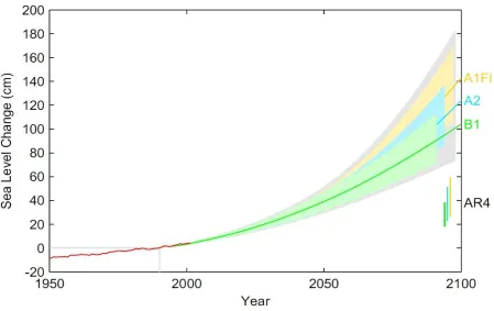
Table 2 shows the GMSL rise in meters with respect to 1986-2005 as projected by the IPCC in AR5. The sum of the projected contributions gives the likely range for future global mean sea level rise. The median projections for GMSL in all scenarios lie within a range of 0.05 m until the middle of the century; the divergence of the climate projections has a delayed effect because oceans take a long time to respond to warmer conditions at the Earth’s surface. However, predicting the behavior of large ice sheets and glaciers is still limited by a lack of understanding of the physical processes and to a lesser degree computing power (Jevrejeva et al., 2012; Vermeer & Rahmstorf, 2009; Walsh et al., 2014). Vermeer & Rahmstorf (2009) realized that AR4 did not include rapid ice flow changes in its projected sea level ranges, arguing that they could not yet be modeled, and consequently did not present an upper limit of the expected rise. In response they proposed a simple relationship linking global sea level variations to global mean temperature.

(26)

18

Figure 6: Projections of sea level rise by Vermeer & Rahmstorf (2009) from 1990 to 2100, based on three different emissions scenarios from the IPCC’s special report on emission scenarios (SRES). The sea level range projected in the IPCC AR4 is shown, for comparison, in the bottom right hand corner (Vermeer & Rahmstorf, 2009).

3.3.2. Regional sea level rise

[image:26.595.74.524.73.356.2]

Regional sea level changes may differ substantially from the global mean sea level rise. Regional factors may cause the local land or sea floor to move vertically and dynamic changes in ocean circulations can cause a local difference in sea level rise as well (Church et al., 2013; N.C. Coastal Resources Commision’s Science Panel in Coastal Hazards, 2010; Parris et al., 2012). Parris et al. (2012) proposed a template for developing regional sea level rise scenarios, see Table 3. Regional sea level change is caused by a combination of three different components: global mean sea level rise, which can be taken from Table 2, and the local vertical land movement and the regional ocean basin trend, both will be discussed in the following two paragraphs.

Table 3: Template for developing regional sea level scenarios(Parris et al., 2012).

Contributing Variables Scenarios of sea level change

RCP 2.6 RCP 4.5 RCP 6.0 RCP 8.5

Global mean sea level rise 22 cm 23 cm 23 cm 25 cm

Vertical Land Movement

(Subsidence or uplift) 1 mm yr

-1

1 mm yr-1 1 mm yr-1 1 mm yr-1 Ocean Basin Trend

(from tide gauges and satellites) 0 mm yr

-1

0 mm yr-1 0 mm yr-1 0 mm yr-1

(27)

19 3.3.2.1. Vertical land movement

Vertical land movement is made up of three components: Glacial Isostatic Adjustment (GIA), any tectonic effect, and the total (net) effect of local processes such as sediment consolidation. However, vertical land movements are primarily associated with GIA (Engelhart, Horton, & Kemp, 2011). GIA is the response of the solid Earth to the changing surface load brought about by the increase and decrease of large-scale ice sheets and glaciers. In the past 20,000 years ice melting and associated GIA have caused up to several hundred meters of relative sea-level rise in different parts of North America (Sella et al., 2007). GIA has been estimated to be 1 mm yr-1 for North Carolina (Engelhart et al., 2011; Kemp et al., 2011). The tectonic component along the Atlantic coast has been widely accepted as being zero or very small and has been constant. The effect of local processes is zero to negligible (Engelhart et al., 2011). The vertical land movement for North Carolina is dependent on the GIA and thus has a magnitude of 1 mm yr-1, the vertical land movement is independent of the RCP scenarios.

3.3.2.2. Ocean Basin Trend

Satellite measurements reveal important variations in the global mean sea level between and within ocean basins. Large scale climate patterns which fluctuate over decades, such as the Pacific Decadal Oscillation (PDO), the North Atlantic Oscillation (NAO), and ENSO, may cause variations in the Pacific Ocean, the Gulf of Mexico, and the Atlantic Ocean (Parris et al., 2012). Research done by Sallenger, Doran & Howd (2012) and Boon (2012) found evidence of accelerated sea level rise for a hotspot along the U.S. Atlantic coast along a 1000 km stretch from Cape Hatteras (North Carolina), to above Boston (Massachusetts). However, for the area south of Cape Hatteras (Beaufort is located roughly 150 km south of Cape Hatteras) the accelerated sea level rise is negligible (Sallenger, Doran, & Howd, 2012).

3.3.2.3. Total regional sea level change

The total regional sea level change for the four RCP scenarios can finally be calculated based on the above mentioned scenarios for global sea level rise (Table 2), vertical land movement and the ocean basin trend. The results for the expected regional sea level changes for each of the climate change scenarios are presented in Table 3.

Hurricanes

3.4.

In chapter 3.2.2 the difference between tropical and extra-tropical cyclones was made. One of the key differences between these two is that tropical cyclones have their strongest winds near the earth's surface , while extra-tropical cyclones have their strongest winds near the tropopause - about 12 km up (Goldenberg, 2004). Because of this difference this paragraph will only assess the climate impacts related to tropical cyclones.

(28)

20

3.4.1. Current North Carolina return period

In order to determine the climate change impacts on hurricanes, the first step is to determine the current hurricane strength associated with storms with return periods of 100 years and 500 years. Appendix B1 shows data regarding all hurricanes that made landfall between the states of Texas and Maine during the 1900-2013 period, as retrieved from the Atlantic Oceanographic & Meteorological Laboratory: Hurricane Research Division (2014). This is the data used in determining the wind speeds that are currently associated with a 100 year storm and a 500 year storm.

This section shows the step by step process of determining the wind speeds that are currently associated with a 100 year storm and a 500 year storm. The current wind speed associated with the 100 year storm is 130 knots or 241 km/h, for the 500 year storm this is 156 knots or 289 km/h. In order to calculate the wind speed associated with the current hurricane return period for North Carolina a number of steps need to be taken, these steps are systematically explained below.

Step 1 – In order to calculate the return periods the hurricane wind speed is required. All hurricanes for which the wind speed at landfall cannot be obtained are removed from the list. This gives Table 4 as an updated version of Table 12 (appendix B1). Table 4: Updated from Table 12 to only show hurricanes for which wind speed can be obtained.

Category Total

Category 1 Hurricanes 80

All Hurricanes 186

Total hurricanes to hit North Carolina 37

Step 2 – The storm categories 1 through 5 are divided into smaller categories to increase the

number of data points. Category 1 starts with the smallest wind speed, 64 knots, and increases with steps of five knots. Some steps have a smaller or larger increase than 5 knots, this is due to the fact that there are fewer than 5 knots remaining within a storm category or the fact that an increment of 5 knots has no storm occurrences. The categories can be viewed in Table 5 (columns 2 and 3).

Step 3 – The number of hurricanes occurring within each of the categories is counted and an

inverse cumulative function is based on the frequency, this can be seen in Table 5 (columns 4 and 5). The inverse cumulative distribution denotes that for a certain category of storms there is a number of storms equal to or greater than the wind speed for this category.

Step 4 – 186 storms have made landfall in the U.S. anywhere from Texas to Maineover a 113

(29)

21

with a certain minimum wind speed, see Table 5 (column 6) for the return periods. 37 out of 192 storms hit North Carolina or 19.27% of storms. The results from column 6 are divided by 0.1927, the result is the return period for North Carolina shown in column 7.

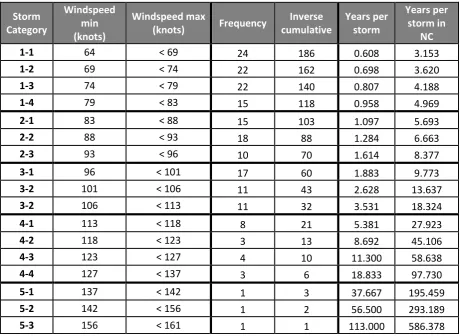
Step 5 – The results from Table 5 column 7 are plotted in Figure 7 (an expanded figure can be found in Figure 32 appendix B2). Based on these computations, the 100 year storm has wind speeds starting at 129.6 knots, the 500 year storm has wind speeds starting at 156.4 knots.

Table 5: Revised storm categories (columns 1,2, and 3), number of storms per category and inverse cumulative distribution of storms (columns 4 and 5), return period for storms in the U.S. and for North Carolina (columns 6 and 7).

3.4.2. Future North Carolina return period

Bender et al. (2010) and Knutson, Sirutis, Vecchi, Garner, & Zhao (2013) explored the influence of future global warming on Atlantic hurricanes with a downscaling strategy. This downscaling method is capable of realistically simulating category 4 and 5 hurricanes. Because the wind speeds associated with the 100 and 500 year storm are a large category 4 and a category 5, this method is applicable to our data as well. This downscaling is based on the ensemble mean of 18 global climate change projections. These 18 models are the result of the World Climate Research Program coupled model intercomparison project 3 (CMIP3) and use the IPCC SRES A1B emissions scenario with global warming for the year 2100. Table 6 shows the results of the downscaling experiments from Bender et

Storm Category

Windspeed min (knots)

Windspeed max

(knots) Frequency

Inverse cumulative

Years per storm

Years per storm in

NC

1-1 64 < 69 24 186 0.608 3.153

1-2 69 < 74 22 162 0.698 3.620

1-3 74 < 79 22 140 0.807 4.188

1-4 79 < 83 15 118 0.958 4.969

2-1 83 < 88 15 103 1.097 5.693

2-2 88 < 93 18 88 1.284 6.663

2-3 93 < 96 10 70 1.614 8.377

3-1 96 < 101 17 60 1.883 9.773

3-2 101 < 106 11 43 2.628 13.637

3-2 106 < 113 11 32 3.531 18.324

4-1 113 < 118 8 21 5.381 27.923

4-2 118 < 123 3 13 8.692 45.106

4-3 123 < 127 4 10 11.300 58.638

4-4 127 < 137 3 6 18.833 97.730

5-1 137 < 142 1 3 37.667 195.459

5-2 142 < 156 1 2 56.500 293.189

[image:29.595.65.526.248.584.2]

(30)

22

al. (2010) and Knutson et al. (2013). These CMIP3 downscaling results will be used to determine the updated frequency of hurricanes under climate change conditions for the year 2050.

Table 6: Downscaling experiments for Atlantic hurricanes, based on comparing 27 Augustus – October seasons (1980-2006) with and without the climate change perturbation for the year 2100 and the year 2050. (Knutson et al., 2013)

Storm category

Ensemble warmed climate 2100 (percent change)

Ensemble warmed climate 2050 (percent change)

Category 1 - 51.6 - 24.3

Category 2 - 17.5 - 8.2

Category 3 - 45.2 - 21.2

Category 4 + 83.3 + 39.2

Category 5 + 200 + 94

This section shows the step by step process of determining the new return periods for North Carolina in the year 2050. The return period for a storm with wind speeds starting at 130 knots (which currently has a return period of 100 years) will become 61 years and the return period for a storm with wind speeds starting at 156 knots (the current 500 year storm) would reduce to only 231 years. The wind speed associated with the current 100 year storm and the current 500 year storm are calculated in section 3.4.1. With the hurricane frequencies changing due to the impacts of climate change, the wind speeds calculated in section 3.4.1 will have a different return period in the future. In order to calculate the new return period associated with the current wind speed for North Carolina a number of steps need to be taken, these steps are systematically explained below.

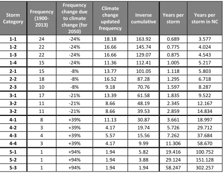
Step 6 – Under climate change conditions the frequency of occurrence for the 5 different hurricane categories will change, Table 6 shows the change in percentage per category of hurricane. The current hurricane frequencies (Table 7 column 2) are updated with the percentage change from column 3 Table 7. Column 4 Table 7 shows the updated frequencies per category.

Step7 – The number of hurricanes occurring within each of the categories is counted and an

inverse cumulative function is based on the frequency, this can be seen in Table 7 (columns 4 and 5). The inverse cumulative distribution denotes that for a certain category of storms there is a number of storms equal to or greater than the wind speed for this category.

Step 8 – 186 storms have made landfall in the U.S. anywhere from Texas to Maineover a 113

year period. Dividing the 113 year period by the number of storms equal to or greater than a certain wind speed yields the return period for a storm with a certain minimum wind speed, see Table 7 (column 6) for the return periods. 37 out of 192 storms hit North Carolina, 19.27% of all storms. The results from column 6 are divided by 0.1927, the result is the return period for North Carolina shown in column 7.

Step 9 – The results from Table 7 column 7 are plotted in Figure 7 (an expanded figure can be

(31)

23

Step 10 – To determine the new return period associated with the wind speeds calculated in step 5, an exponential trend line is added to the data points. The wind speed from step 5 is used in combination with the trend line to determine the new corresponding return period. The old 100 year storm with wind speeds of 129.6 knots has a return period of 61 years under climate change conditions by the year 2050. The old 500 year storm with wind speeds of 156.4 knots has a return period of 231 years under climate change conditions by the year 2050.

Table 7: Number of storms per category, number of storms per category with climate change, and inverse cumulative distribution of storms (columns 2,3, and 4), return period for storms in the U.S. and for North Carolina (columns 5 and 6).

Storm Category

Frequency

(1900-2013)

Frequency change due

to climate change (for

2050)

Climate change updated frequency

Inverse cumulative

Years per storm

Years per storm in NC

1-1 24 -24% 18.18 163.92 0.689 3.577

1-2 22 -24% 16.66 145.74 0.775 4.024

1-3 22 -24% 16.66 129.07 0.875 4.543

1-4 15 -24% 11.36 112.41 1.005 5.217

2-1 15 -8% 13.77 101.05 1.118 5.803

2-2 18 -8% 16.52 87.28 1.295 6.718

2-3 10 -8% 9.18 70.76 1.597 8.287

3-1 17 -21% 13.39 61.58 1.835 9.522

3-2 11 -21% 8.66 48.19 2.345 12.167

3-2 11 -21% 8.66 39.53 2.859 14.834

4-1 8 +39% 11.13 30.87 3.661 18.997

4-2 3 +39% 4.17 19.74 5.726 29.712

4-3 4 +39% 5.57 15.56 7.262 37.684

4-4 3 +39% 4.17 9.99 11.306 58.670

5-1 1 +94% 1.94 5.82 19.416 100.752

5-2 1 +94% 1.94 3.88 29.124 151.128

[image:31.595.67.521.222.573.2]

(32)

24

Figure 7: North Carolina hurricane return period. Wind speed plotted against the return period. 1

10 100 1,000

60 70 80 90 100 110 120 130 140 150 160

R

e

tu

rn

p

e

ri

o

d

(year

s)

Windspeed (knots)

North Carolina Return period current

(33)

25

4. Risk perception

Divided into three subjects, risk will be explored by taking a look at objective risk, subjective risk, and the way risk is incorporated into the RHEA model. The objective risk shows the actual risk. The subjective risk goes into the theory of how housing market actors observe risk. Both kinds of risk will be addressed in this chapter. This chapter concludes by showing how risk perception bias (i.e. subjective risk) has been added to the RHEA model.

Objective risk

4.1.

Within this research objective risk is defined as the actual flood risk probability, the Federal Emergency Management Agency (FEMA) is responsible for determining the flood risk probability in the United States. In accordance with the National Flood Insurance Program (NFIP) FEMA defines geographical areas according to varying levels of flood risk. Three different types of flood zones can be defined for the coastal area: (i) high risk zones, coastal areas with a 1:100 flood probability; (ii) moderate risk zones, coastal areas with a 1:500 flood probability; and (iii) low risk zones, coastal areas determined to be outside of the 1:500 probability flood zone (Michel-Kerjan, 2010). The latest flood maps for Beaufort have been created in 2003.

For Carteret County the dominant source of flooding are wind driven storm surges associated with hurricanes (Carteret County, n.d.). For Beaufort no other source of flooding could be determined. The assumption is made that under current conditions a hurricane with a return period of a 100 years is responsible for flooding the 1:100 flood zone and a hurricane with a return period of 500 years would be responsible for the flooding of the 1:500 flood zone (section 3.4.1.). The return periods and associated flooding probabilities under climate change conditions have been determined in section 3.4.2.

Subjective risk

4.2.

Housing market actors will assess objective flood risk on the basis of probability and severity of damage, these are biased by myopia and amnesia. Under these two principles it could mean that subjective risk can diverge considerably from objective risk, especially if a long time has passed since a local flood event has occurred. In this section the principles of myopia and amnesia, and the housing market response to these principles will be discussed.

4.2.1. Myopia

Myopia is the discounting of information for anticipated future events. The discounting will rise progressively as the event becomes less anticipated (Pryce et al., 2011). Four main reasons exist why it can be expected that information regarding the future will be discounted.

(34)

26

in the distant future. Second, the public has a tendency to distrust the information about the future since they believe these are attempts by vested interests to exert power (Pryce et al., 2011) and they might just disagree with what scientists are telling them (Kahan, Jenkins‐Smith, & Braman, 2011). Third, climate models are highly technical and their outcomes are probabilistic. Limited understanding leads to an inability of people to respond appropriately to data in terms of density functions and dependent scenarios. Finally, purchasing a house does not occur under ceteris-paribus conditions. Buying a house is a process riddled with emotions, hopes, ambitions, and imagined lifestyle aspirations on which the dangers of future flooding have little influence (Pryce et al., 2011).

4.2.2. Amnesia

In contrast to myopia, amnesia is the discounting of information from past events, with the discount rising progressively as time elapses. Households weigh recent flood information more heavily than they do with floods that happened a long time ago, the risks of flooding will be overestimated right after a flood but declines quickly as time passes without re-occurring flood events (Pryce et al., 2011). The cognitive effects of flooding disappear within a 5 to 6 year period (Bin & Landry, 2013). An important consideration in this respect is the difference between individual amnesia and market amnesia. Even though individual households might be perfectly aware of flood risks potential buyers coming from outside the area may not be. Information asymmetry may be exacerbated by home owners and real estate agents who conceal flood risks in an attempt to stop the reduction in property values (Pryce et al., 2011).

4.2.3. Housing market response to myopia and amnesia

In this section, we will take a look at the housing market response to flood risk under myopia and amnesia. Figure 8 serves as a starting point, it depicts an efficient housing market with fully risk-adjusted prices. Figure 8 shows how floods at tF1 and tF2 only have a temporary effect on observed

property values (PA). This holds true for a particular area in which the market valuations are fully

(35)

27

Figure 8: Fully risk-adjusted prices and short-run responses to flooding (Pryce et al., 2011)

Figure 9 shows a world of imperfect information. In this situation the house price will drift from the risk adjusted house price to the zero risk house price in the years following a flood event, due to changing subjective risk as a result of myopia and amnesia. When a flood event occurs, the market will suddenly become aware of the flood risk and adjust the house price downward to the risk adjusted house price. It is even possible in the immediate aftermath of a flood for future flood risks to be overestimated, leading to a drop below the (objective) risk adjusted house price.

Figure 9: House prices with myopia and amnesia (adapted from Pryce et al., 2011)

Risk perception bias procedure

4.3.

(36)

28

bias. In order to do this, the RHEA model is extended. This addition can be found in appendix D2. This part of the code will allow for risk perception bias to be related to a flood event. Three new variables have been introduced in the risk perception bias code to allow the myopia and amnesia to be incorporated into the RHEA model, their functions are discussed below.

“counter” – The counter counts the time steps that have passed since a flood event. From Pryce et al. (2011) and Bin & Landry (2013) we find that people ‘forget’ what has happened after a period of five years, the current counter has been set to count 10 semi-annual time steps for a total of five years. The counter is reset when a flood event has happened.

“perception_change” – Right after a flood event the perception of risk will be highest and as a result the property values at this time will be the lowest, as can be seen in Figure 9. With perception_change the individual risk perception bias can be set for the time right after a flood event.

“DC” – The discount coefficient allows the perception_change to be discounted over 10 time steps from a state of maximum risk perception bias to a state of ‘zero risk’. This parameter represents the gradual decrease of the risk perception bias when time since the latest flood passes.

From Bin & Landry (2013) we saw that the discount factor follows a logarithmic curve, so it was decided that the risk perception bias should also have a logarithmic curve. In Figure 10 we see the logarithmic curve used for discounting.

Figure 10: Logarithmic discount coefficient curve providing discount coefficients for calculating perceived flood risks after a flood event.

The perception code functions as follows.

1. The procedure checks if the counter has a value of <= 10, if this is not the case, the A-RPbias is set to zero since the assumption is made that people live in a ‘zero risk’ world (Pryce et al., 2011). The current procedure assumes that it takes five years for the risk perception bias to recover and reach ‘zero risk’ perception.

0.00 0.10 0.20 0.30 0.40 0.50 0.60 0.70 0.80 0.90 1.00

1 2 3 4 5 6 7 8 9 10

D

isco

u

n

t

co

e

ff

ic

ie

n

t

(37)

29

2. The procedure checks if ‘sameRPbias’ is set to true, if this is the case A-RPbias will be the same for everybody. In this case A-RPbias is determined by taking the value for DC for the right time step and is multiplied with perception_change.

3. If ‘sameRPbias’ is false, the calculation for A-RPbias takes an extra step. The curve from Figure 10 is used, again with the value assigned to the slider ‘perception_change’. A normal distribution of A-RPbias is assumed with:

a. Mean (DC * perception_change)

b. Standard deviation ((DC * perception_change) * (1/6))

The A-RPbias is normally distributed and randomly assigned to agents, and uses a mean which is equal to the A-RPbias if ‘sameRPbias’ is set true, as seen in step 2.

(38)

30

5. Scenario analysis

This chapter will start with the definition of the scenarios that will be used in the simulations with the RHEA model. Next the results of these simulations will be displayed and analysed. The analysis of these results will serve as the basis for the discussion and conclusion in the subsequent chapters, aiming to answer the research objective.

Scenarios

5.1.

In order the quantify the effect of climate change, associated flood risks and risk perception bias on coastal urban property values, four scenarios have been developed to be simulated using the RHEA model. The four scenarios allow for varying between climate change and steady-state climatic conditions, and for differentiating between market participants with perfect information and the ones whose risk perceptions are biased. Each scenario simulates a period of about 50 years, from 2003 until 2050. The choice for 2003 as a starting point has been made because the current flood maps and associated flood risks have last been updated by FEMA in 2003. In order to be able to incorporate risk perception bias, a flood event has to happen to start the risk perception bias procedure (section 4.3). To achieve this, two flood events have been added, one after 10 semi-annual time steps (5 years) and one after 60 semi-annual time steps (30 years) from the start of the simulation.

5.1.1. Scenario 1

The first scenario serves as a baseline scenario, applying steady-state climatic conditions and accounting for objective risks only. the traders in the RHEA model operate under perfect information and assume the original (objective) flooding probabilities of 0.01 for the 100 year floodplain and 0.002 for the 500 year floodplain. Scenario 1 allows to simulate the development of property values without the interference of risk perception bias or climate change.

5.1.2. Scenario 2

In the second scenario the traders again operate under perfect information (objective risk only). However, this time traders assume the flooding probabilities will be increasing due to the impacts of climate change (section 3.4.2). This scenario therefore applies flooding probabilities of 0.0164 for the current 100 year floodplain and 0.0043 for the current 500 year floodplain. Scenario 2 allows to simulate the development of property values under climate change without risk perception bias.

5.1.3. Scenario 3

In the third scenario, climatic conditions are again assumed steady, but traders no longer operate in a world of perfect information. Instead they operate under the risk perception bias as it was determined in chapter 4.2. Scenario 3 allows to simulate the development of property values under risk perception bias, but without climate change.

5.1.4. Scenario 4

(39)

31

Table 8: An overview of the four scenarios to be simulated using the RHEA model

Climate Change

No Yes

Risk perception bias

No Scenario 1 Scenario 2 yes Scenario 3 Scenario 4

Results

5.2.

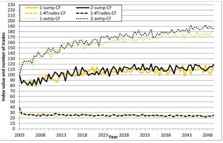
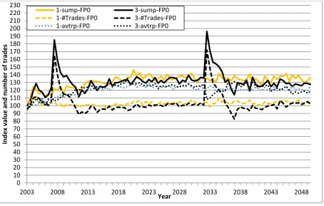
In this section, the results from the scenario simulations will be presented and analysed. Each scenario has been simulated with a total of 16 different random seeds , each representation of data will be the average of these 16 random seeds. The input parameters for each scenario are the same and can be found in appendix C2. For each scenario, four different flood zones are monitored, these are: the safe zone (FP0), the current 100 year floodplain without the coastal front properties (FP100noCF), the current 500 year floodplain (FP500), and the coastal front properties (CF). For each flood zone three statistics are monitored: the number of trades in each time step for every flood zone (#Trades), the total value of the trades in each time step for every flood zone (sump), and the average trade price in each time step for every flood zone (avtrp). Each result displayed here will be accompanied by a code to keep track of what it represents, these codes will be formatted as follows, ‘1-sump-FP100noCF’. The code is made up of three parts that are separated by a dash (-): the first part shows the scenario number, the second part the statistic being tracked, and the final part determines the flood zone at stake.

The properties in the current 100 year floodplain and the coastal front properties were separated from each other because the coastal front properties are on average 2 to 3 times more expensive than non-coastal front properties in the 100 year floodplain. By separating these two zones, it is possible to get a better representation of the development of property values in the 100 year floodplain.

All the figures showing results have been formatted in the same way, this makes comparison between graphs easier. The x-axis shows the time in the simulation and ranges from the year 2003 to the year 2050. The y-axis is uniform for all graphs with a range of 0 to 230. The y-axis has 2 meanings, first, for the total value of trades (sump) and the average trade price (avtrp) it shows indexed values, expressed as a percentage of the value of the first time step. Second for the number of trades (#Trades) it shows the number of trades.

5.2.1. The Impact of climate change on property values under perfect

information

In order to determine the effects of climate change on property values in Beaufort, scenarios 1 and 2 are compared. With both scenario 1 and 2 operating under perfect information (objective risk only) the results allow to visualize the effect of climate change without the influence of risk perception bias.

Quantifying the impacts of climate driven flood risk changes and risk perception biases on coastal urban property values ; A case study for the North Carolina coastal zone