Proceedings of the Institution of Civil Engineers
Geotechnical Engineering 161
June 2008 Issue GE3 Pages 137–149
doi:10.1680/geng.2008.161.3.137
Paper 700049
Received 03/08/2006 Accepted 05/09/2007
Keywords:
concrete structures/mathematical modelling/tunnels & tunnelling
Benoıˆt D. Jones
Engineering Manager, Morgan Est Plc, Rugby, UK
Alun H. Thomas
Senior Engineer, Mott MacDonald, Croydon, UK
Yu Sheng Hsu
Senior Geotechnical Engineer, Mott MacDonald, Croydon, UK
Matousˇ Hilar
Senior Tunnel Engineer, D2 Consult, Prague, Czech Republic (formerly of Mott MacDonald)
Evaluation of innovative sprayed-concrete-lined tunnelling
B. D. Jones
MEng, EngD, A. H. Thomas BA, PhD, CEng, MICE, Y. S. HsuBEng, PhD, ACGIand M. Hilar
MSc, PhD, CEng, MICEThe front-shunt tunnel was the first tunnel of the Terminal 5 project at Heathrow to be constructed, and was the first section of sprayed-concrete-lined (SCL) tunnel to be constructed using the method known as LaserShell. This innovation represented a significant deviation from the methods previously used in SCL construction. Therefore it was subjected to a careful examination before and during construction using sophisticated 3D numerical modelling and monitoring during construction. The paper presents typical results from surface settlement levelling,
inclinometers and extensometers, pressure cells and tunnel lining displacement measurements, and comments on the performance of the methods and instruments used. The paper then presents the methodology and typical results of the numerical modelling, and shows that the predictions of displacements and stresses compared well with the field measurements. In terms of the control of ground deformations and structural safety the tunnel performed well.
NOTATION
c cohesion of sprayed concrete
Ehtan horizontal tangent Young’s modulus
Ei initial tangent Young’s modulus of sprayed concrete
Evtan vertical tangent Young’s modulus
Gtan tangent shear modulus
Ktan tangent bulk modulus
p9 mean effective stress
r correlation coefficient
å current strain of the sprayed concrete
åa axial strain
åi strain in Cartesian directioni
åpk strain at peak strength of sprayed concrete
åv volumetric strain
Poisson’s ratio
ó stress
óc unconfined compressive strength of sprayed concrete
ót tensile strength of sprayed concrete
óy yeild stress
angle of friction of sprayed concrete
1. INTRODUCTION
The front-shunt tunnel, a 40 m long and 4.15 m internal dia. tunnel boring machine (TBM) launch chamber for the stormwater outfall tunnel (SWOT), was the first tunnel of the
Terminal 5 (T5) project at Heathrow to be constructed. More importantly, the frontshunt was the first section of sprayed concrete lined (SCL) tunnel to be constructed using the method known as LaserShell.
The method (described in detail by Williamset al.1) represented
a significant deviation from the methods previously used in SCL construction. The face was inclined at an angle of
approximately 708to the horizontal to provide a protective
canopy for operatives close to the face, and a laser surveying system was used to control the shape of the excavation and lining, obviating the need for operatives to enter the face to measure the excavation or install lattice girders (Fig. 1). Therefore the method was subjected to careful examination before and during construction. During the ‘definition design stage’ of the work the tunnelling contractor carried out a comprehensive programme of testing to identify the optimum
concrete mix and hone the construction methodology.2The
lead designer reviewed the detailed design provided by the
3 6 m– 1 m 1 m 1 m
Previous advances
75 mm initial layer
200 mm primary layer 50 mm finishing layer
Approx. 0·5 m Stagger of
joints: Layers of
sprayed concrete:
Primary layer
[image:1.595.310.553.486.757.2]Initial layer
contractor’s designer, and this review included advanced
numerical modelling using FLAC3D. The predictions of
behaviour provided by the numerical modelling, together with consideration of many other issues, led to this innovative method of construction being accepted by the client for use on all the SCL tunnels for the T5 project. The paper presents the methodology and results of this modelling.
Mott MacDonald’s role on site was to oversee technical compliance and safety. The paper presents typical results of monitoring during construction, which included surface settlement levelling, three-dimensional (3D) tunnel lining displacement monitoring, subsurface instruments
(extensometers and inclinometers), and tunnel lining pressure cells. The performance of the instrumentation is then discussed, and the results are compared with the results of the advanced numerical modelling.
2. LOCATION AND INSTALLATION OF INSTRUMENTS
The location and layout of instrumentation is shown in Fig. 2. Surface settlement was monitored using levelling points, and ground movements were monitored using inclinometers and extensometers grouted into boreholes. Tunnel lining displacements were monitored by 3D optical surveying of targets. Ground pressure on the tunnel lining was measured using radial pressure cells, and stresses in the sprayed concrete lining were measured using tangential pressure cells. Typical results and comments on the usefulness and accuracy of the instrumentation are presented below.
2.1. Surface settlement levelling points
The grid pattern of settlement points for the tunnel was extensive: it included 97 points (Fig. 2). Two arrays were installed adjacent to the shaft, and ten arrays of points were installed across the tunnel axis. The spacing of the settlement points was generally 7 m in the longitudinal direction (spacing between each transverse array) and 5 m in the perpendicular direction (spacing between the points in a transverse array). In
general, accuracy was in the range1 mm. The settlement
data were zeroed at the end of shaft construction, so the results presented show only the effect of the frontshunt tunnel construction. Shaft construction took eight weeks, and then there was a delay of a further four weeks before the frontshunt tunnel excavation began. During this four-week delay ongoing settlements continued for up to a week and then stabilised. Furthermore, there were no discernible ongoing settlements due to shaft construction at the points to the north-east, south-west and north-west of the shaft during frontshunt construction (see Fig. 2).
Surface settlements when the face was directly under each transverse array (1–6) are shown in Fig. 3. These show an approximately Gaussian settlement pattern; for comparison a curve for a volume loss of 0.28% and a trough width parameter
kof 0.5 (Peck3) has been added to Fig. 3. Array 1 showed a
slight heave rather than settlement, but this is within the accuracy of the surveying, and so all that can be concluded is that negligible movement occurred. As the tunnel moved further from the shaft, settlements increased, and by the time the face was under array 3—about 15 m or three tunnel
SWOT front-shunt tunnel
SWOT inlet shaft
Ar
ra
y 1
Ar
ra
y 2
Ar
ra
y 3
Ar
ra
y 4
Ar
ra
y 5
Ar
ra
y 6
Ar
ra
y 7
Ar
ra
y 8
Ar
ra
y 9
Ar
ra
y 10
ar
ra
y 1
Pressure cells
ar
ra
y 2
Pressure cells
5
55
5
5
10
7 7 7 7 7 7 7 7
5
5
10
6
6
2
6
8
8
3
8 5
5 5 4
Surface settlement monitoring point
Inclinometer
Combined extensometer/ inclinometer
2
46
47 43
44
45
48 01
8 6
[image:2.595.44.538.432.755.2]Site roads
diameters from the shaft—the settlements stabilised where the influence of the shaft was negligible.
The settlement trough for array 3 was skewed to the left (north of the tunnel centreline), with an anomalous large settlement at
10 m in Fig. 3, array 4 had a larger settlement over the
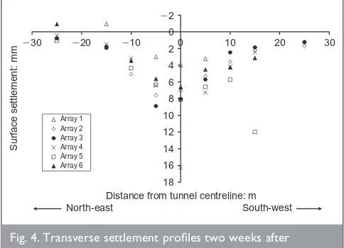
tunnel centreline than the other arrays, and array 5 had an unexpectedly large settlement of 10 mm at 15 m to the right (south) of the tunnel centreline. This phenomenon is also evident in Fig. 4, which shows the surface settlement at the same locations two weeks after construction of the frontshunt tunnel had finished. This was probably caused by the traffic of cranes and muck lorries over these locations. The plan in Fig. 2 shows that these points lay in the site road, so heavy traffic causing additional settlement would seem the most likely
explanation. The settlement point10 m from the tunnel
centreline in array 3 was damaged shortly after the reading in Fig. 3 was taken, and so no data were available for this point in Fig. 4.
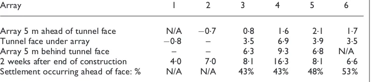
The centreline settlements when the tunnel face was under each settlement array, and the centreline settlements two weeks after construction had ceased (denoted ‘Final’ in Fig. 5), are shown in longitudinal section in Fig. 5. These data are summarised in Table 1, together with the settlements when each array was 5 m ahead of the tunnel face and 5 m behind
the tunnel face. Fig. 5 and Table 1 show that ahead of the face, even at 5 m distance, very little surface settlement was observed. The stabilised maximum settlement, ignoring the local effect that caused an anomalous reading at array 4, was approximately 8 mm. The percentage of settlement occurring ahead of the tunnel face for arrays 3 to 6 is shown in the last row of Table 1, found by dividing the cumulated settlement in the second row by the final cumulated settlement in the fourth row. Array 6 had the greatest value of 53% because the tunnel ended only 4 m beyond the array. The typical value for continuous tunnelling from array 3 to 5 was around 45%.
2.2. Inclinometers and extensometers
Two inclinometer boreholes and five combined inclinometer and extensometer boreholes were installed in the positions shown in Fig. 2.
Readings from inclinometer 48 are shown in Fig. 6. Since the base of the inclinometer was 7.6 m below the invert of the tunnel, it was assumed that the base was fixed. The average standard deviation of baseline horizontal movements measured by the total station surveying of the top of the instrument casing was 2.5 mm, implying a 95% confidence of repeatability
within5 mm, and no obvious movement either towards or
away from the face of the tunnel could be identified. Therefore whole-body translations and rotations of the inclinometer could not be estimated, but were probably of small magnitude relative to the horizontal movements at tunnel depth. Van der Berget al.4assumed that the top of the inclinometers installed at Heathrow Terminal 4 station in London Clay were fixed in
the longitudinal direction. Nyrenet al.5measured longitudinal
horizontal surface movements of up to 8 mm at St James’s Park, although this was in the context of much larger ground movements—approximately three times larger than at the SWOT. It is thought unlikely, therefore, that inclinometer 48 could have undergone a whole-body rotation such that the top of the instrument moved more than 3 mm horizontally.
Fixing the displacement at either the top or the base of the
inclinometer resulted in a scatter of the readings of2 mm at
the opposite end owing to accumulated errors along the length of the inclinometer. Therefore, in the interpretation, it was
assumed that the baseandthe top of the inclinometer were
fixed, in order to minimise these accumulated errors. Very little movement occurred until the tunnel face was less than 4 m
South-west North-east
⫺2 0 2 4 6 8 10 12 14 16 18
Distance from tunnel centreline: m
Surface settlement: mm
Face under array 1 Face under array 2 Face under array 3 Face under array 4 Face under array 5 Face under array 6 Gaussian curve
[image:3.595.59.297.41.206.2]⫺30 ⫺20 ⫺10 0 10 20 30
Fig. 3. Transverse settlement profiles when tunnel face was under array 1 to array 6. Gaussian curve based onVl¼0.28% andk¼0.5
⫺2 0 2 4 6 8 10 12 14 16 18
Distance from tunnel centreline: m
Surface settlement: mm
Array 1 Array 2 Array 3 Array 4 Array 5 Array 6
South-west North-east
[image:3.595.313.553.43.203.2]⫺30 ⫺20 ⫺10 0 10 20 30
Fig. 4. Transverse settlement profiles two weeks after construction
Chainage along centreline: m
Settlement: mm
Face at array 1 Face at array 2 Face at array 3 Face at array 4 Face at array 5 Face at array 6 Final ⫺2
0 2 4 6 8 10 12 14 16 18
0 5 10 15 20 25 30 35 40
Array 1 Array 2 Array 3 Array 4 Array 5 Array 6
[image:3.595.56.298.589.764.2]from the inclinometer. The recorded movements before this were indicative of the accuracy of the inclinometer, and were
generally within2 mm—similar to the accuracy reported by
van der Berget al.4The maximum horizontal movement was
11 mm when the last reading was taken and the face was 0.9 m from the inclinometer.
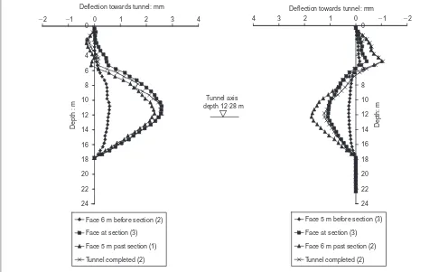
Readings from inclinometers 44 and 46, offset 6 m from the tunnel centreline, are shown in Fig. 7. The inclinometers were approximately 3.5 m from the extrados of the tunnel at its closest point. They measured very little horizontal movement in the ground—of the order of less than 3 mm. As mentioned
previously, the repeatability was approximately2 mm, and so
these movements were barely outside the accuracy of the instrument. The top of the inclinometer was assumed fixed but there may have been a small horizontal movement towards the tunnel at the surface. At the Heathrow Express trial tunnel,
Deane and Bassett6measured horizontal surface movements at
approximately 2.4 radii distance from the tunnel centreline (the
same number of radii distance as inclinometers 44 and 46) to be approximately 5 mm. This was 26% of the horizontal movement at the tunnel axis depth. Applying the same ratio to
inclinometers 44 and 46, the surface horizontal movement of the inclinometers would have been less than 1 mm.
The readings from extensometer 43 on the tunnel centreline are shown in Fig. 8. The extensometer data were adjusted
according to the settlement of the top of the instrument casing measured by precise levelling. The tunnel axis was at 12.13 m depth at this location. Very little subsurface movement occurred while the tunnel approached the instrument, although some was discernible in magnet B, which was located about 3.4 m above the crown of the tunnel. The instrument casing and surrounding grout were mined through as the tunnel passed, but the extensometer was removed just prior to this.
Figure 9 shows the subsurface vertical movements measured by extensometer 44, 6 m offset from the tunnel centreline. In this case, the extensometer could be continuously read as the tunnel passed, and vertical movements were greater than those measured by extensometer 43. The accuracy of the
extensometer measurement when the tunnel face was
substantially far away (.20 m) to influence the readings was
2 mm. The deepest magnets A and B showed no discernible
movement. Magnet C, located at about the same level as the tunnel axis, showed a downward vertical movement, as did magnets D and E between the tunnel crown level and the surface.
2.3. Convergence monitoring
Conventional monitoring of the lining was achieved using a 3D optical surveying technique to measure convergence of the lining. Seven arrays were installed approximately 5 m apart, each with five convergence targets (left knee, left shoulder, crown, right shoulder and right knee), shown in Fig. 10. During the driving of the tunnel there were continual problems with the placing of the targets, and many targets were damaged and had to be replaced. This resulted in a large amount of lost information. In general, measurements in the frontshunt tunnel
showed noise of2–3 mm, which, according to Bock,7is
typical for this method of surveying under these conditions.
2.4. Pressure cells
Twenty oil-filled pressure cells were placed in two arrays in the tunnel, the first 8 m into the tunnel and the second 28 m into the tunnel. In each array, pressure cells were placed in five positions: left knee, left shoulder, crown, right shoulder and
right knee, equally spaced with an angle of approximately 728
between them. At each position, two pressure cells were placed: a radial ‘earth’ pressure cell and a tangential ‘sprayed concrete’ pressure cell. Also, two tangential pressure cells were placed in
a 1000 mm31000 mm3300 mm test panel, which was
sprayed at the same time as array 2 and kept for the first month at the bottom of the SWOT inlet shaft. This meant it was
0
2
4
6
8
10
12
14
16
18
20
22
24
Deflection in direction of tunnel drive: mm
Depth: m
16·7 m (2)* 14·7 m (2) 12·7 m 8·7 m 4·7 m (3) 3·7 m 1·7 m 0·9 m (2) Distance from tunnel face to inclinometer:
Tunnel axis level
* Brackets denote number of readings averaged
[image:4.595.48.413.41.122.2]⫺15 ⫺10 ⫺5 0 5 10 15
Fig. 6. Readings from inclinometer 48 on tunnel centreline (positive deflection is away from the face)
Array 1 2 3 4 5 6
Array 5 m ahead of tunnel face N/A 0.7 0.8 1.6 2.1 1.7
Tunnel face under array 0.8 – 3.5 6.9 3.9 3.5
Array 5 m behind tunnel face – – 6.3 9.3 6.8 N/A
2 weeks after end of construction 4.0 7.0 8.1 16.3 8.1 6.6 Settlement occurring ahead of face: % N/A N/A 43% 43% 48% 53%
[image:4.595.43.279.180.506.2]exposed to the same environmental conditions as the tunnel pressure cells.
The array 2 radial pressure cell data are shown in Fig. 11. Cells 558 and 560, the crown and right knee radial pressure cells, have been omitted because the recorded pressures dropped below zero owing to temperature changes. Therefore they temporarily lost contact, and did not record pressure changes over a significant period of time. There was a period of approximately six months between late February and early September where no readings could be taken because the junction box was sited behind the conveyor installed for the TBM drive, and no automatic data acquisition system was provided.
0
2
4
6
8
10
12
14
16
18
20
22
24
⫺2
⫺1 0 1 2 3 4
Deflection towards tunnel: mm
Depth: m
Face 5 m before section (3)
Face at section (3)
Face 6 m past section (2)
Tunnel completed (2) 0
2
4
6
8
10
12
14
16
18
20
22
24
Deflection towards tunnel: mm
Depth : m
Face 6 m before section (2)
Face at section (3)
Face 5 m past section (1)
Tunnel completed (2)
⫺2 ⫺1 0 1 2 3 4
Tunnel axis depth 12·28 m
Fig. 7. Deflection of inclinometers offset 6 m from the tunnel centreline (positive deflection is towards the tunnel): (a) inclinometer 46 (offset to left); (b) inclinometer 44 (offset to right). (Brackets denote number of readings averaged; inclinometer head and base assumed fixed)
⫺10
⫺8
⫺6
⫺4
⫺2 0 2 4
0 5
10 15
20 25
Tunnel face distance from extensometer: m
V
e
rtical mo
v
ement: mm
Magnet A: 23·159 m depth Magnet B: 6·361 m depth Magnet C: 2·305 m depth NB: tunnel axis at 12·28 m depth
Fig. 8. Extensometer 43 movements as tunnel face approached
⫺10
⫺8
⫺6
⫺4
⫺2 0 2 4
⫺20
⫺15
⫺10
⫺5 0 5 10 15 20
Tunnel face distance from extensometer: m
V
e
rtical mo
v
ement: mm
Magnet A: 18·69 m depth Magnet B: 16·30 m depth Magnet C: 12·30 m depth Magnet D: 8·24 m depth Magnet E: 4·31 m depth
[image:5.595.56.552.42.343.2]NB: tunnel axis at 12·28 m depth
Fig. 9. Extensometer 44 movements (6 m offset from centreline) as tunnel face approached and passed
1
2
4
3
5
[image:5.595.60.551.382.773.2]On 12 February 2003 the radial pressure cells were crimped. Crimping involves crushing the crimping tube using a specially made crimping tool. This forces a fixed amount of hydraulic oil into the pressure cell cavity in order to prevent loss of contact between the pressure cell and the medium in which it is embedded. It is not clear whether radial pressure cells should be crimped at all. If they are well installed, there is no reason
why they should lose contact.8Also, crimping will effectively
jack the surface of the pressure cell against the London Clay. Since London Clay is a saturated porous medium, this will generate excess pore pressures and, in time, consolidation will occur. These crimping pressures were found to dissipate within two weeks and so have not been removed from the dataset.
The ground pressure acting on the sprayed concrete lining after nine months at array 2 was between 126 and 155 kPa at an
average temperature of 158C: that is, between 53% and 65% of
the hydrostatic full overburden pressure at tunnel axis level (239.9 kPa). The pressures in Fig. 11 are dependent on temperature, as expansion and contraction of the sprayed concrete ring increases and decreases the radial pressure between the ground and the sprayed concrete lining. Therefore the effect of temperature on radial pressure cells should not be removed, since it represents a true change in the ground pressure acting on the tunnel lining. These results were
presented in detail by Jones.9
The tangential pressure cell data are not presented in this paper owing to insufficient space; there is no technical reason for their omission.
3. NUMERICAL MODEL
The innovative construction method demanded the use of an explicit 3D numerical model, since the unique features of the construction method could not be represented in a semi-empirical 2D model or analytical solution and be differentiated from standard construction methods. Key concerns were the influence of early-age loading, the sloping face, and the
staggered joints. It was decided to use FLAC3Dbecause of the
ease with which non-linearity and plasticity of the soil and sprayed concrete could be implemented.
The numerical modelling results presented in this paper may be considered as a prediction, even though this particular analysis was undertaken after construction. The objective was not to change the ground parameters until the ground movements were perfectly predicted but to check the validity of the prediction with the as-built geometry. The original analyses used for the design were adjusted only in the following ways.
(a) The tunnel diameter was increased from 4.8 m to 5.0 m and
the primary lining thickness increased from 0.2 m to 0.275 m to take account of the over-excavation of at least 0.1 m observed during construction.
(b) The London Clay horizon and water table locations were
adjusted to the levels encountered during construction. The London Clay horizon was found at 4.44 m below the surface. The water table was found at 1.0 m below the surface.
(c) The depth to tunnel axis was increased from 11.8 m to
12.28 m.
(d) The advance rate was set to 3.3 m/day.
(e) The undrained shear strength profile was changed from the
design values, which represented a lower bound to the site investigation data, to a best fit of the site investigation data.
3.1. Tunnel geometry and excavation sequence
In order to model the construction method reasonably
accurately, the following steps were taken. The tunnel face was
inclined at an angle of 718to the horizontal (Fig. 12). The
sprayed concrete lining was placed in two layers: an initial layer 75 mm thick, which was installed up to 1 m from the face, followed by a primary layer 275 mm thick, installed to within 1.67 m of the face. The tunnel was circular, with an excavated diameter of 5.0 m. To reduce boundary effects an initial length of 32 m was excavated, 60% of the initial ground stress was allowed to dissipate at the tunnel perimeter, and the lining was installed. Subsequently the tunnel was excavated in 1 m advance lengths, with the lining installed after each advance.
0 50 100 150 200 250 300 350
Date
R
e
ad pressure: kP
a
0 5 10 15 20 25 30 35
T
e
mper
a
ture: °C
Cell 556 left knee Cell 557 left shoulder Cell 559 right shoulder Hydrostatic full overburden Cell 557 temperature
558 557 559
556 560
[image:6.595.43.282.37.271.2]04/02/03 05/04/03 04/06/03 03/08/03 02/10/03
Fig. 11. Radial pressure cells at array 2
London Clay
Terrace Gravel
72 m 57 m
Plastic zone
Primary layer Initial
layer
1 m 0·67 m 71°
60 m
[image:6.595.296.540.547.757.2]3.2. Ground properties
The geological profile adopted in the model comprised 4.44 m of Terrace Gravel overlying the London Clay, which extended to a depth of 60 m. The geotechnical parameters for each of the strata are listed in Table 2. The water table was taken to be 1 m below ground level, with a hydrostatic pore pressure
distribution through the Terrace Gravel and the London Clay.
Back-analysis of previous excavations at Heathrow has demonstrated that an anisotropic soil model with a higher stiffness in the horizontal plane best represents the behaviour
of the London Clay.10,11However, the anisotropic model
implemented in FLAC3Dwas purely elastic, and did not permit
yielding of the soil. Since plastic behaviour may be important when modelling the tunnel lining–ground interaction, an isotropic elastic perfectly plastic model was adopted for the London Clay within a tunnel radius distance of the periphery of the tunnel, and an elastic anisotropic model was adopted for the London Clay and the Terrace Gravel in the remainder of the
model. This approach was used by Scottet al.11and was found
to be effective. The pre-peak non-linearity of the Terrace Gravel and the London Clay was modelled broadly following
the method suggested by Jardineet al.,12as adapted by Scottet
al.11for isotropic and anisotropic materials in 3D using
effective stresses. The equations are given in Appendix 1.
During the analysis, the stiffness of both the isotropic and anisotropic soils was updated every ten calculation steps as a compromise between accuracy and calculation time. This
resulted in an error of5% when compared with updating the
stiffness at every step in a model that simulated triaxial compression and extension.
The initial in situ stress profile and the undrained shear strength profile for the London Clay applied in the model were based on the site investigation data, and are shown in Fig. 13.
TheK0value for the Terrace Gravel was taken to be 0.4. The
K0values used were obtained from suction probe
measurements on pushed thin-walled tube samples, as
described by Hightet al.13
3.3. Sprayed concrete properties
A programme of laboratory tests was carried out on the sprayed concrete mix to determine its full stress–strain curve at an age of less than one day. The results of this testing were
reviewed, and a curve based on the BS 8110 Part 214stress–
strain equation was fitted to the data, as shown in Appendix 2.
The design rate of unconfined compressive strength development is shown in Table 3.
A strain-hardening Mohr–Coulomb material model was used for the sprayed concrete. Thus the level of plastic strain was used to calculate the stress at every calculation step for values
of stress between the yield stressóyand the compressive
strengthóc. The yield stressóywas assumed to be equal to 0.4
times the compressive strength. Details of the Mohr–Coulomb model are given in Appendix 2.
Similarly, a curve was fitted to a graph of initial tangent Young’s modulus against compressive strength, and the values in Table 4 were obtained for use in the analysis.
Parameter Terrace
Gravel
London Clay
Bulk unit weight: kN/m3 19.5 20.0
Porosity: % 35 50
Cohesion: kPa 0 134 + 10z*
Friction: degrees 38 0
Dilation: degrees 0 0
[image:7.595.312.552.42.545.2]Young’s modulus: MPa Variable Variable Poisson’s ratio Variable Variable * Undrained shear strength for London Clay, wherezis depth from top of London Clay.
Table 2. Geotechnical properties
0
5
10
15
20
25
Depth: m
0 1 2 3
K0
(a)
0 100 200 300 400
cu: kPa
0
5
10
15
20
25
Depth: m
(b)
4. DISCUSSION
4.1. Surface settlement
The design prediction of surface settlements used the empirical
method based on a Gaussian curve.3The volume loss was
assumed to be 1.1%, and a trough width parameterkof 0.45
was used. This value of volume loss was based on an upper bound of volume losses measured during the construction of previous SCL tunnels in London Clay at Heathrow, in particular the Heathrow Express tunnels, and is shown in Fig. 14. The SWOT frontshunt tunnel had a considerably lower volume loss than this, and Fig. 14 shows that a curve based on a volume loss of 0.63% and a trough width parameter of 0.5 fits the data better, at least in terms of the maximum settlement over the
centreline. However, further away from the tunnel centreline the trough appears to be wider than the Gaussian curve predicts. Indeed, the volume losses calculated by direct trapezoidal integration of the settlement data were 0.97%, 1.09% and 1.10% for arrays 3, 4 and 5 respectively. In order to match these volume losses with a maximum settlement of 8 mm, a trough width
parameterkof between 0.8
and 0.9 would be required. The width of the trough may have been caused by ongoing local consolidation
settlements: less than a month before construction began at least 1 m of fill was placed over the whole site.
The numerical modelling overpredicted the maximum settlement, at 13.5 mm compared with 8 mm
measured in the field. The volume loss predicted by FLAC3D
was 1.47%. Although this volume loss may appear high, this was due largely to the width of the settlement trough predicted. The overprediction of maximum settlement may indicate that the stiffness of the soil was underestimated in the model, but the narrower settlement trough observed in the field indicates perhaps that some element of ground behaviour was not modelled correctly.
Comparing the longitudinal settlement profile with the FLAC3D
[image:8.595.42.411.41.150.2]analysis (Fig. 15) shows that the predicted pattern of settlements agrees reasonably well with the observed behaviour. The larger observed settlements over the tunnel centreline at array 4 are evident. These data were omitted from Fig. 14 since they were due to heavy traffic movements, and were not indicative. As noted before, the numerical analysis resulted in larger settlements over the excavated tunnel than were observed in reality at arrays 3, 5 and 6, and the final settlements when construction finished were also
overpredicted.
Prediction of surface settlement is often used as the main measure of success of a numerical model, although the key design parameter is the stress in the lining. Negro and de
Queiroz15reviewed 65 papers on numerical modelling of
tunnels. Of the 55 papers that compared predicted maximum surface settlement with measured values, 39 of the predictions,
corresponding to more than 70%, were within10% of the
measured values. Shirlaw and Wen16questioned the accuracy
of comparisons made between measured surface settlements and those predicted by numerical methods. They pointed out that the natural variations in settlements were generally much
higher than10%, and suggested that this contradiction may
exist because few people would publish cases where the
Age Sprayed concrete design strength,óc: MPa
Age Sprayed concrete design strength,óc: MPa
0 h 0.0 3 days 25.0
0.1 h 0.2 5 days 28.0
1 h 0.5 7 days 30.0
3 h 1.0 10 days 31.5
6 h 3.0 15 days 33.0
12 h 8.0 20 days 34.0
1 day 15.0 28 days 35.0
Table 3. Sprayed concrete design strength development
Unconfined compressive strength: MPa
Initial tangent Young’s modulus,
Ei: GPa
Unconfined compressive strength:
MPa
Initial tangent Young’s modulus,
Ei: GPa
0.10 0.003 2.56 2.5
0.15 0.008 3.84 4.0
0.22 0.022 5.77 5.4
0.34 0.060 8.65 7.0
0.50 0.150 13.00 8.5
0.76 0.350 19.50 10.5
1.14 0.800 29.20 12.0
[image:8.595.42.413.198.332.2]1.70 1.500 43.80 14.0
Table 4. Development of initial tangent Young’s modulus with compressive strength
30 20
10 0
⫺10
⫺20
0
2
4 6
8
10 12
14
16
⫺30
Distance from tunnel centreline: m
Surface settlement: mm
Array 3 Array 4 Array 5 Gaussian fit
0·63%, = 0·5
Vl⫽ k
Gaussian curve 1·1%, = 0·45
Vl⫽ k
FLAC3D
Fig. 14. Comparison of surface settlements from site two weeks after tunnel construction with FLAC3Dand empirical
[image:8.595.42.283.568.738.2]predicted and actual settlements were significantly different, or because ‘predictions’ may have been made after the event and adjusted to match performance. In addition, if settlements were measured at several locations, the ‘typical’ profile may have been selected carefully. With this in mind, the predictions presented in this paper were acceptable, given the small magnitudes of the settlements.
4.2. Subsurface ground movement
Figure 16 shows selected data from inclinometer 48 on the tunnel centreline compared with corresponding data from
FLAC3D. The inclinometer data have been adjusted to fit the
FLAC3Ddata at 1 m and 20 m depth, since whole-body
translations and rotations of the inclinometer could not be measured. For small movements, when the tunnel face was
about 5 m away from the inclinometer, the FLAC3Dpredictions
matched the measured behaviour reasonably well. However, closer to the tunnel face, where larger movements occurred, the numerical analysis overestimated the movements. This may have been caused by the isotropic model around the tunnel, which would have had a lower horizontal stiffness than the anisotropic London Clay has in reality. The patterns of deformations predicted were similar to those observed, except just below the invert level of the tunnel, where small
deformations towards the tunnel face were measured that were not predicted.
Figure 17 shows the data from inclinometers 44 and 46 offset 6 m from the tunnel centreline compared with corresponding
data from FLAC3D. The inclinometer data were adjusted for this
figure in the same way as for inclinometer 48 in Fig. 16. Since the variability of the field data, as illustrated by the difference between the movements of inclinometers 44 and 46, was relatively high, the numerical modelling cannot be expected to perfectly match the data. The numerical modelling did overpredict the magnitude of the movements, but the pattern of movements was replicated well. It is likely, given that the surface settlements were overpredicted by the numerical modelling, that the main reason for the discrepancy was a general overprediction by the model owing to the lack of anisotropy close to the tunnel.
Figure 18 shows the movements of magnet D of extensometer 44 offset 6 m from the tunnel centreline compared with the
numerical modelling prediction. Magnet D was approximately
1.5 m above the crown level of the tunnel, and the FLAC3D
data were taken from a gridpoint 1.3 m above the crown level, offset 6 m from the tunnel axis. The movements in front of the face were predicted well by the numerical modelling but the movements after the face had passed were overpredicted. This may also be seen in the surface settlements above the tunnel centreline shown in Fig. 15.
4.3. Tunnel lining deformations
The vertical movements of the tunnel crown at different locations are plotted in Fig. 19. Most of the movement occurred within the first seven days of the tunnel construction, and varied between 4 and 8 mm. The tunnel crown
displacements predicted by FLAC3Dwere calculated
immediately after the excavation. In reality, however, the first reading was taken some time after excavation because the sprayed concrete layer had to be applied before convergence targets could be installed. The first readings were usually taken within 12 h. Therefore initial movements were not recorded. To
account for this fact, the curve from the FLAC3Dprediction has
been adjusted by subtracting the initial displacements of the lining before the subsequent advance was excavated. Fig. 19 shows that the numerical modelling prediction was good. The prediction stopped at six days in Fig. 19 because of the limited length of the model.
Claytonet al.8have questioned the ability of lining
convergence measurements to give adequate warning of excessive stresses in an SCL. They recommended ensuring that
Array 6 Array 5
Array 4
5 6
40 35 30 25 20 15 0
2 4 6 8 10 12 14 16 18
10
Chainage along centreline: m
Settlement: mm
Face at array 3 Face at array 4 Face at array 5 Face at array 6 Final FLAC3D Array 3
3
4
[image:9.595.315.552.43.364.2]F
Fig. 15. Comparison of longitudinal FLAC3Dresults with settlements along centreline. For FLAC3Dresults, number denotes array under which face is located; F denotes final short-term settlement two weeks after construction
5 0
⫺5 –10
⫺15 0
2
4
6
8
10
12
14
16
18
20
22
24
⫺20
Deflection in direction of tunnel drive: mm
Depth: m
4·7 m (average of 3 readings) 0·9 m (average of 2 readings) FLAC3D5 m
FLAC3D1 m
Distance from tunnel face to inclinometer 48:
Tunnel axis level
Fig. 16. Adjusted inclinometer 48 data compared with FLAC3D; on tunnel centreline (positive deflection is away
[image:9.595.57.302.43.187.2]the accuracy of the measurement system is at least an order of magnitude less than the estimated convergence at compressive failure of the completed SCL ring. The measurement system employed at this site would have failed to provide this. Despite the shortcomings of convergence measurements in this type of
SCL tunnel, Claytonet al.8made the important point that
increasing convergence following ring closure would still indicate a manifestation of problems with the completed SCL, and therefore it remains important to record convergence measurements. The convergence measurements made at this site were appropriate for this purpose.
4.4. Tunnel lining loads
The radial pressure cells recorded radial stresses equal to 53– 65% of hydrostatic full overburden pressure. This range of values was broadly in line with the previous measurements of ground load on 4–5 m diameter segmentally lined tunnels in
London Clay17of 40–60% of the overburden pressure at one
year after installation. It was also broadly in line with previous radial pressure cell measurements in SCL tunnels: for instance in the Terminal 4 station platform tunnels of 30–50% of full
overburden pressure,18at Redcross Way of 30%,19and in the
Terminal 4 concourse tunnel of 34–78%.9
The low radial pressures and the concomitant low volume loss show that no benefit would have been gained from allowing the ground to deform more by delaying the closure of the tunnel lining at the invert. Previous tunnels in London Clay with higher volume losses have generally had much higher radial pressures.
The FLAC3Dmodel did not include the effects of temperature
changes on the sprayed concrete lining during hydration. This was the cause of the large discrepancy shown in Figs 20 and
21 during the first few days. In the long term, FLAC3D
underpredicted the radial stress, predicting 80–85 kPa (equal to 33–35% of hydrostatic full overburden pressure at tunnel axis level).
The pressure cell readings therefore revealed a phenomenon that had not been considered during the design: the effect of temperature changes—and hydration heat in particular—on the ground pressure acting on the lining. Immediate closure of the ring of sprayed concrete, although resulting in smaller volume losses, will also expose the sprayed concrete lining to the highest potential stresses at early age of up to 100% of the
0
2
4
6
8
10
12
14
16
18
20
22
24
0 2 4 6 8
Deflection towards tunnel: mm
Depth: m
Inclinometer 44 Inclinometer 46 FLAC3D
[image:10.595.296.540.42.334.2]Tunnel axis level
Fig. 17. Adjusted inclinometer 44 and 46 data compared with FLAC3D; 6 m offset from tunnel centreline after tunnel face
has passed section by at least 5 m
⫺8
⫺6
⫺4
⫺2 0 2 4
⫺20
⫺15
⫺10
⫺5 0 5 10 15 20
Tunnel face distance from extensometer: m
V
e
rtical mo
v
ement: mm
Magnet D: 8·24 m depth FLAC3D
Fig. 18. Extensometer 44 magnet D data compared with FLAC3Dprediction
25 20
15 10
5
⫺2
0
2
4
6
8
10 0
Time: days
Crown settlement: mm
[image:10.595.42.281.51.388.2]FLAC3D FLAC3Dadjusted Chainage 30 Chainage 35 Chainage 40
[image:10.595.41.283.451.588.2]hydrostatic overburden pressure. This occurred at 10–15 h after spraying. However, consideration of the interpolated design strength at 10 h (see Table 3) and the design thickness of 275 mm results in a factor of safety of 3 at this time, so the sprayed concrete lining was never overstressed.
4.5. Numerical modelling
Since many papers have been published on the subject of the behaviour of SCL tunnels in London Clay, and the authors’ organisation has been involved in the design and supervision of a large number of SCL and segmentally lined tunnels constructed in London Clay, the numerical modelling was informed by a large body of experience and previous back-analyses. The predictions of ground deformations made by the
FLAC3Dmodel were reasonable. The level of sophistication of
the model exemplified by the complexity of the constitutive models and the detailed geometry represent current best practice in the tunnelling industry, but did not require specialist computer hardware or excessive run times.
Even if great care is taken in the gathering and interpretation of field data, field measurements will be subject to variations, mainly because of the variability of the material properties and the accuracy of the instrument, and so predictions can never exactly match the field data at all locations. Many published papers quote comparisons between predictions and field data implying an accuracy that is better than this natural variability should allow.
In this case, the patterns of ground movement (at the surface and below ground), lining deformation and loading were predicted well by the numerical model, but there is scope for improvement. Most notably, ground movements close to the tunnel were overpredicted. However, it is noteworthy that a good agreement was achieved across the whole spectrum of ground and lining deformations and lining stresses.
5. CONCLUSIONS
The SWOT front-shunt was constructed using an innovative SCL method. To provide assurance of the suitability of this method, it was thoroughly investigated during the design phase using sophisticated 3D numerical models, and during
construction an extensive array of instrumentation was installed in and around the tunnel to record the behaviour of the tunnel and the ground. Despite some difficulties in the monitoring, a valuable set of data was obtained that was used to produce an informative case history. All the information gathered from the instrumentation was useful, providing the client with confidence in the ability of the method to control ground deformations and confirming that the design predictions were reasonable.
In general, the pattern of behaviour of the ground was consistent with observations of other SCL tunnels in London Clay. The performance of the tunnelling method in controlling ground movements, with a volume loss of 0.63%, was at the lower end of the range of previous experiences of SCL tunnelling in London Clay. The deformations of both the ground and the lining were small, and stabilised quickly. The tight control of deformations was achieved mainly by the relatively early ring closure in the full-face excavation.
The radial ground pressures on the tunnel lining stabilised quickly at a relatively low value, and showed no inclination to increase in the long term. In general, tunnels with higher volume losses in London Clay have also experienced higher radial pressures, so it should generally be considered good practice to keep deformations as small as possible in London
08/02/03 07/02/03
06/02/03 05/02/03
0 50 100 150 200 250 300 350
04/02/03
Time
R
adial stress: kP
a
0 5 10 15 20 25 30 35
T
emper
a
ture: °C
Cell 557 Cell 559
Hydrostatic full overburden FLAC3D
[image:11.595.57.297.38.322.2]Cell 557 temperature
Fig. 20. Radial pressures at shoulder level compared with FLAC3Dradial stresses
08/02/03 07/02/03
06/02/03 05/02/03
0 50 100 150 200 250 300 350 400
04/02/03
Time
R
adial stress: kP
a
0 5 10 15 20 25 30 35 40
T
emper
a
ture: °C
Cell 556 Cell 560 FLAC3D
Hydrostatic full overburden Cell 556 temperature
Fig. 21. Radial pressures at knee level compared with FLAC3D
[image:11.595.57.296.377.666.2]Clay. The pressure cells also revealed that hydration
temperatures may bring about the worst-case loading at early age in a shallow full-face SCL tunnel.
Opinion is sometimes divided about the merits of numerical modelling in design. In this case the 3D numerical model provided good predictions of behaviour explicitly: that is, without induction. Any other design method in this case would have comprised an empirical element and assumptions about behaviour or geometry that might or might not have been appropriate. The numerical model described in this paper achieved a good agreement with the field measurements in the ground and lining in terms of both deformations and stresses. Sophisticated modelling of both the ground and the sprayed concrete lining was essential to this success.
6. APPENDIX 1. SMALL-STRAIN STIFFNESS EQUATIONS
Ktan¼ p9 RþScosðºYÞ
SºY1
ln 10 sinºY
ð Þ
whereY ¼log10 åv
T 1
Gtan¼
p9
3 AþBcosÆX
ª
ð Þ BªÆXª
1
ln 10 sinÆX
ª
ð Þ
whereX¼log10 åa
C 2
whereR,S,T,º,,A,B,C,Æandªare constants, the values
of which are given in Table 5;Ktanis the tangent bulk
modulus;Gtanis the tangent shear modulus;p9is the mean
effective stress;åvis the volumetric strain; andåais the axial
strain. Since the original equations by Jardineet al.12were
based on an undrained triaxial test,åawas obtained from the
FLAC3DCartesian strain tensor using the relationship
åa¼ ffiffiffi 2 p
3 [(åxåy)
2þ(å
yåz)2þ(åzåx)2
þ6(å2
xyþå2yzþå2zx)] 1 2 3
The shear and bulk moduli reduce with shear and volumetric strains respectively.
The anisotropic model had five independent elastic parameters.
The vertical and horizontal Young’s moduli and the shear modulus varied with shear strain, as described by the following equations.
Evtan¼ p9 AþBcosðÆXªÞ
BªÆXª1
ln 10 sinÆX
ª
ð Þ
4
Ehtan¼1:6Evtan 5
Gvhtan¼ Evtan
2:4
6
hh¼0:2 7
hv¼0 8
7. APPENDIX 2. SPRAYED CONCRETE MODEL EQUATIONS
The stress–strain curve was based on the following equations
from BS 8110 Part 2.14
ó¼óc
k2
1þðk2Þ
" #
9a
¼ å åpk 9b
k ¼åpkEi óc 9c
whereEiis the initial tangent Young’s modulus,åpkis the
strain at peak strength,åis the current level of strain, andócis
the unconfined compressive strength.
The angle of frictionin the strain-hardening Mohr–Coulomb
model was taken to be 37.438, and the angle of dilation was
taken to be zero. The cohesion was related to the stress by the relationship
A B C Æ ª åamin åamax
Terrace Gravel 1100 1050 9.03106 1.22 0.75 9.03106 2.03103
London Clay 770 730 7.03106 1.338 0.684 7.03106 1.53103
R S T º åvmin åvmax
Terrace Gravel 275 225 2.83105 1.1 1.0 3.03105 7.03103
[image:12.595.44.541.637.755.2]London Clay 150 100 4.93105 2.0 1.0 5.03105 8.013104
c¼ó 1sin
2cos
10
A curve was fitted to the strain at peak strength data from the tests, and the following relationship was found with a
correlation coefficientr2¼0.81.
åpk¼0:0136ó0
:47
c 11
The sprayed concrete density was 2.4 Mg/m3. Poisson’s ratio
was assumed to remain constant at a value of 0.2. The tensile strength of the sprayed concrete was given by the relationship
ót¼0:3ó0
:67
c 12
ACKNOWLEDGEMENTS
The authors would like to acknowledge the kind permission of Ian Williams on behalf of BAA in permitting this paper to be published. They would also like to acknowledge the
contribution of many individuals, both on site and in the design office, to the successful construction of the tunnel and the gathering of the monitoring data. The analysis of the pressure cell data by Benoıˆt Jones was supported by the EPSRC and the University of Southampton, supervised by Professor Chris Clayton.
REFERENCES
1. WILLIAMSI., NEUMANNC., JA¨ GERJ. and FALKNERL.
Innovativer Spritzbeton-Tunnelbau fu¨r den neuen Flughafenterminal T5 in London (Innovative shotcrete tunnelling for London Heathrow’s new Terminal 5). Proceedings O¨ sterreichischer Tunneltag 2004, Salzburg, 2004, 41–61.
2. HILARM., THOMASA. H. and FALKNERL. The latest
innovation in sprayed concrete lining: the LaserShell
method.Tunel(Magazine of the Czech Tunnelling
Committee and the Slovak Tunnelling Committee ITA/ AITES), 2005, 4, 11–19.
3. PECKR. B. Deep excavations and tunnelling in soft ground.
Proceedings of the 7th International Conference on Soil
Mechanics and Foundation Engineering, Mexico, 1969,
State-of-the-art report, 225–290.
4. VAN DERBERGJ. P., CLAYTONC. R. I. and POWELLD. B. Displacements ahead of an advancing NATM tunnel in the
London Clay.Ge´otechnique, 2003,53, No. 9, 767–784.
5. NYRENR. J., STANDINGJ. R. and BURLANDJ. B. Surface
displacements at St James’s Park greenfield reference site
above twin tunnels through the London Clay. InBuilding
Response to Tunnelling: Case Studies from Construction of the Jubilee Line Extension, London. CIRIA, London, 2001, Vol. 1, pp. 387–400.
6. DEANEA. P. and BASSETTR. H. The Heathrow Express trial
tunnel.Proceedings of the Institution of Civil Engineers,
Geotechnical Engineering, 1995,113, No. 3, 144–156.
7. BOCKH. Geotechnical instrumentation of tunnels. In
Summerschool on Rational Tunnelling(KOLYMBASD. (ed.)).
Logos Verlag, Berlin, 2003, pp. 187–224.
8. CLAYTONC. R. I., HOPEV. S., HEYMANNG.,VAN DERBERG
J. P. and BICAA. V. D. Instrumentation for monitoring
sprayed concrete lined soft ground tunnels.Proceedings of
the Institution of Civil Engineers, Geotechnical Engineering,
2000,143, No. 3, 119–130.
9. JONESB. D. Measurements of ground pressure on sprayed
concrete tunnel linings using radial pressure cells.
Proceedings of Underground Construction 2005, London,
2005 (CD-ROM).
10. CHANGJ., SCOTTJ. M. and POUNDC. Numerical study of
Heathrow cofferdam.Proceedings of the 2nd International
Symposium FLAC and Numerical Modeling in
Geomechanics, Lyon, 2001, 163–169.
11. SCOTTJ. M., POUNDC. and SHANGHAVIH. B. Heathrow
Airside Road Tunnel: wall design and observed
performance.Proceedings of the International Conference
on Underground Construction, London, 2003, pp. 281–292.
12. JARDINER. J., POTTSD. M., FOURIEA. B. and BURLANDJ. B.
Studies of the influence of non-linear stress–strain
characteristics in soil–structure interaction.Ge´otechnique,
1986,36, No. 3, 377–396.
13. HIGHTD. W., GASPARREA., NISHIMURAS., MINHN. A.,
JARDINER. J. and COOPM. R. Characteristics of the London
Clay from the Terminal 5 site at Heathrow Airport. Ge´otechnique, 2007,57, No. 1, 3–18.
14. BRITISHSTANDARDSINSTITUTION.Structural Use of Concrete.
Code of Practice for Special Circumstances. BSI, London, 1985, BS 8110 Part 2.
15. NEGROA. andDEQUEIROZP. I. B. Prediction and
performance: a review of numerical analyses for tunnels. Proceedings of the International Symposium Geotechnical Aspects of Underground Construction in Soft Ground, Tokyo, 2000, pp. 409–418.
16. SHIRLAWJ. N. and WEND. Checking and reviewing the
output from numerical analysis.Proceedings Underground
Singapore 2005, Singapore, 2005, 241–249.
17. MAIRR. J. and TAYLORR. N. Theme lecture: Bored
tunnelling in the urban environment.Proceedings of the
14th International Conference on Soil Mechanics and Geotechnical Engineering, Hamburg, 1997,4, 2353–2385.
18. POWELLD. B., SIGLO. and BEVERIDGEJ. P. Heathrow
Express: design and performance of platform tunnels at
Terminal 4.Proceedings of Tunnelling ’97, London, 1997,
565–593.
19. KIMMANCEJ. P. and ALLENR.. The NATM and compensation
grouting trial at Redcross Way.Proceedings of the
International Symposium on Geotechnical Aspects of
Underground Construction in Soft Ground, London, 1996,
pp. 385–390.
What do you think?
To comment on this paper, please email up to 500 words to the editor at journals@ice.org.uk