cow-path problem with a non-optimal
seeker
G
abi
M
aduro
s
1101706
University of Twente [email protected],
April 6, 2018
1.
I
ntroduction
In computer science, search problems are extensively studied problems. A well-known search problem is thecow-path problem, which was first known as thelinear search problem. The cow-path problem was introduced by Richard Bellman(Bellman 1963), and independently studied by Anatole Beck(Beck 1964) and Wallace Franck (Franck 1965). It plays an important role in many applications of computer science and also comes up in artificial intelligence applications(Kao et al. 1996). The name of the cow-path problem comes from the following scenario: Somewhere on a line, referred to as the origin, there is a seeker: a cow, named Bessie. Bessie is searching for a special flower to eat, which is located somewhere on the line at distanced≥1 from the origin. To find this flower, Bessie is moving on the line and has the choice to walk either to the right or to the left, leading her off into unknown territory. The goal is to minimize the costs(in this case the distance Bessie has to walk before she finds the flower). Bessie is blind unfortunately and will only find the flower if she touches it. Bessie does not know how far away the flower is located and on which side it is located, but she knows it is somewhere on the line.
Previous work looked at the competitive ratio of algorithms used for the cow-path problem. The
competitive ratiois defined as the worst-case ratio of the distance travelled by the algorithm and the shortest possible distance to the goal. In different ways it is proven that the optimal deterministic strategy to solve the cow-path problem has a competitive ratio of 9. So when the hidden item is located at distancedfrom the origin, the distance travelled by the algorithm never exceeds 9d. Beck & Newman (1970), found this ratio of 9, looking at the cow-path problem from a game theory perspective. Baeza-Yates et al. (1993) proved that there is no better ratio than 9 and that their algorithm, which they named thelinear spiral search, is optimal for the deterministic case. With the linear spiral search the seeker alternates between going left and right and doubles the maximum distance to the origin after each iteration. Fuchs et al. (2003) look at a more general problem and give a different proof for the optimality of the competitive ratio of 9 for the cow-path problem. Gal (1974) looked at a more general variant of the cow-path problem, called thestar searchor the
w-lane cow-path problem. In the scenario described as abovew=2, where in thew-lane cow-path problem Bessie is standing at the crossroads ofwpaths which she can walk on to find the goal. Gal (1974) showed that it is optimal to visit each path periodically with monotonically increasing step sizes. Kao et al. (1996) came up with an optimal randomized algorithm for the original cow-path problem, giving a competitive ratio of 4.5911. Kao et al. (1996) show that this randomized algorithm is also optimal for thew-lane cow-path problem.
(2006) investigated the cow-path problem with turning costs for example. Jez & Łopusza ´nski (2009) investigated a 2d variant of the cow-path problem where Bessie has to find a fence that is either a horizontal or vertical line. This variant is different from the 4-lane cow-path problem, since the seeker is not restricted to search on 4 different paths, but can search anywhere in the 2d-plane. Another example is the research of Spieser & Frazzoli (2012), where several cows search for an object on the unit circle.
In spite of all this research, there has been done very little research on the second problem Richard Bellman stated in his article(Bellman 1963): What if the seeker misses the goal with a certain probablity p > 0? Searching with an non-optimal seeker will be the main topic of this paper. Heukers (2017) already took a look at this problem using the linear spiral search algorithm and later optimizing the algorithm. Instead of doubling the maximum distance to the origin after an iteration, (Heukers 2017) used a factora>1 to find the goal in the average-case scenario using a non-optimal seeker.
Now for small values of pit is intuitive that there must be better algorithms than multiplying the distance by a certain factor in the different direction compared to the origin after an iteration, because missing the hidden item means travelling a great distance before a chance of finding it again. In this paper we first continue on the work of Heukers (2017) looking for new algorithms in the average-case scenario, then we investigate the influence of the non-optimal seeker for the expected travel distance and finally there will be simulations, testing if the theoretic upper bounds for the expected travel distance match the outcomes of the simulations.
2.
T
he
A
verage
-
case scenario
As explained in the introduction, this paper studies a non-optimal seeker, searching for an item on a line. In this section two new algorithms are introduced, optimized and compared to known algorithms for the average-case scenario.
Definition 2.1. In the average-case scenario we assume that the seeker finds the item after hit-ting it for theEthtime, whereE=l1pm.
The distance from the origin to the item will be denoted by d ≥ 1. We try to minimize the distance travelled by the seeker. The seeker starts his search at a certain point, the origin. As soon as he hits the item, he will find it with probabilityp>0. Since we are interested in the number of times hitting the item before finding it, we use a geometric distribution. The expected number of times hitting the item until finding it is thenE= 1p. So, on average the seeker will find the item after hitting itEtimes. IfE∈/N,Eis rounded up to the nearest integer.
For the average-case scenario, we define an iterationjto end when the seeker returns to the origin and starts travelling in the opposite direction. To describe the distance travelled in an iterationj, the function fj =aj−1,∀j≥1,a>1 is used, where fj is the maximum distance to the origin in iterationj. Clearly,amust be greater than one, else the seeker only searches in the interval[−1, 1]. Heukers (2017) also looked at the average-case scenario and used an algorithm using the same function fj described as above. This algorithm will be called thestandard factoralgorithm in this paper and does the following: In every iteration the seeker will start at the origin. The seeker will then travel fj in the opposite direction(compared to the iteration before) and then back to the origin. Heukers (2017) showed that in the average-case scenario the competitive ratios for the standard factor algorithm are 2aa−E+11 −1 forEis even and 2aa−E+11 +1 forEis odd. The competitive ratios for the standard factor algorithm are optimal fora=1+pin the average-case scenario. With this algorithm the point where the item is located, is visited two times in a certain iterationj. Then it will visit this point again two times in iterationj+2, again without finding it ifEis large. Since the distance in each iteration gets larger each time by a factora>1 it seems more efficient to travel more back and forth in one iteration before returning to the origin. We define the interior of the interval visited after an iterationjas thesegmentcorresponding to iterationj. The interior of the visited interval is taken, because we want to say something general on how many times each point in segmentjafter an iteration jis visited. For the algorithms used in this paper, the borders of the visited interval will be visited substantially less than the points lying in the interior of the interval.
2.1.
Algorithm 4times
2.1.1 Competitive ratio 4times
Theorem 2.1. The competitive ratio of 4times for the average-case scenario is 4aE−a1−−12aE−3 −1if E is even and 4aE−a1−−21aE−3 +1if E is odd.
Proof. In the worst case, the distancedfrom the origin to the item is fi+e, where fi=ai−1and e>0 is some small number. Then the travel distance of algorithm 4times for the average-case scenario is:
2· i+E−2
∑
j=1
(2· fj−fj−2) + (−1)E+1d.
Thus, there are two cases to be distinguished: E is even andE is odd. If Eis even, the travel distance is:
2· i+E−2
∑
j=1
(2·fj−fj−2)−d=2·
i+E−3
∑
j=0
(2·aj−aj−2)−d
=4·a
i+E−2−1 a−1
−2·a
i+E−4−1 a−1
−ai−1−e
=4a
E−1−2aE−3 a−1 −1
·ai−1− 2 a−1−e
≤4a
E−1−2aE−3 a−1 −1
(fi+e)
=4a
E−1−2aE−3 a−1 −1
·d. IfEis odd, the travel distance is:
2· i+E−2
∑
j=1
(2·fj−fj−2) +d=2·
i+E−3
∑
j=0
(2·aj−aj−2) +d
=4·a
i+E−2−1 a−1
−2·a
i+E−4−1 a−1
+ai−1+e
=4a
E−1−2aE−3 a−1 +1
·ai−1− 2 a−1+e
≤4a
E−1−2aE−3 a−1 +1
(fi+e)
=4a
E−1−2aE−3 a−1 +1
·d.
So, the competitive ratio for the cow-path problem with a non-optimal seeker for the average-case scenario is 4aE−a1−−21aE−3 −1 ifEis even, and 4aE−a1−−21aE−3 +1 is odd.
2.2.
Algorithm Etimes
Visiting each point of segmentjat least four times can still be too little, ifEis large. Algorithm
Etimesis then introduced for a more general case. The idea of this algorithm is the same as the idea of algorithm 4times, only now every point on segment jhas been visited at leastEtimes. Note that when the seeker returns to the origin, every point in the segment, except, for the origin
must have been visited an even number of times. So when E is even this does not give any complications. However whenEis odd, we need to decide if we visit each point of segmentjat leastE−1 orE+1 times. For now, all three cases will be looked at, later in this paper both cases for whenEis odd will be compared.
Algorithm Etimes does the following in iteration j: First travel to fj in the opposite direction compared to the iteration before, travelE−2 times,E−1 orE−3 times back and forth between
fj−2and fj, depending on whetherEis odd or even, and finally return to the origin. 2.2.1 Competitive ratio Etimes
Theorem 2.2. The competitive ratio of Etimes for the average-case scenario is bounded by Ea3−a(E−1−2)a−1
if E is even, (1+E)aa3−−1(E−1)a −2a2+1if E is odd and the seeker visited each point of segment j at least E+1times and (E−1)aa4−−(E1 −3)a2 +1if E is odd and the seeker visited each point of segment j at least E−1
times.
Proof. In the worst case, the distancedfrom the origin to the item is fi+e, where fi=ai−1and e>0 is some small number. Then the travel distance of algorithm Etimes for the average-case scenario must be looked at for three different cases. Case 1,Eis even:
i+2
∑
j=1
2· fj+ (E−2)(fj−fj−2)
−d= i+1
∑
j=0
2·aj+ (E−2)(aj−aj−2)−ai−1−e
=E· i+1
∑
j=0
aj−(E−2) i+1
∑
j=0
aj−2−ai−1−e
=E·a i+2−1
a−1
−(E−2)·a i−1 a−1
−ai−1−e
=Ea
3−(E−2)a a−1 −1
·ai−1− 2 a−1−e
≤Ea
3−(E−2)a a−1 −1
(fi+e)
=Ea
3−(E−2)a a−1 −1
·d. IfEis odd and the seeker visits each point of segmentjat leastE+1 times: i+2
∑
j=1
2· fj+ (E−1)(fj− fj−2)
−(2fi+2−d) =
i+1
∑
j=0
2·aj+ (E−1)(aj−aj−2)−(2ai+1−d)
= (E+1) i+1
∑
j=0
aj−(E−1) i+1
∑
j=0
aj−2−(2ai+1−d)
= (E+1)a i+2−1
a−1
−(E−1)a i−1 a−1
−(2ai+1−ai−1−e)
=(1+E)a
3−(E−1)a a−1 −2a
2+1·ai−1− 2 a−1 +e
≤(1+E)a
3−(E−1)a a−1 −2a
2+1
(fi+e)
=(1+E)a
3−(E−1)a a−1 −2a
IfEis odd and the seeker visits each point of segmentjat leastE−1 times: i+3
∑
j=1
2· fj+ (E−3)(fj− fj−2)
+d= i+2
∑
j=0
2·aj+ (E−3)(aj−aj−2)+d
= (E−1) i+2
∑
j=0
aj−(E−3) i+2
∑
j=0
aj−2+d
= (E−1)a i+3−1
a−1
−(E−3)a i+1−1
a−1
+ai−1+e
=(E−1)a
4−(E−3)a2 a−1 +1
·ai−1− 2 a−1+e
≤(E−1)a
4−(E−3)a2 a−1 +1
(fi+e)
=(E−1)a
4−(E−3)a2 a−1 +1
·d.
So, the competitive ratio of Etimes for the average-case scenario is bounded by Ea3−a(E−1−2)a−1 ifE
is even, (1+E)aa3−−1(E−1)a−2a2+1 ifEis odd and the seeker visited each point of segmentjat least
E+1 times and (E−1)aa4−−(E1 −3)a2 +1 ifEis odd and the seeker visited each point of segmentjat leastE−1 times.
2.3.
Comparing the standard factor algorithm to 4times and Etimes
In this subsection the performance of the algorithms will be compared according to the competitive ratios calculated in the previous subsections. First is tried to optimize the competitive ratios according toa, such that the competitive ratios can be compared for different values ofp. For the algorithm Etimes there are two competitive ratios whenEis odd, depending on how often the seeker travels back and forth on the interval(fj−2,fj)in each iterationj. In this subsection will be shown for whichpwhich case of the algorithm is optimal and will be used.
2.3.1 Optimizing the algorithms for a
For all algorithms in this paper the distance function fj=aj−1,∀j≥1,a>1 is used to describe the distance travelled by the algorithms. For each algorithm a competitive ratio is calculated which is dependent on the factoraand on the probability p.
Heukers (2017) showed that for the standard factor algorithma=1+pis an optimal value fora. This leads to an optimal competitive ratio for the standard factor algorithm of 2(1+p)
1
p+1
p + (−1) 1
p+1 which is dependent on the probabilityponly.
In this research is tried to optimize the competitive ratios in the same way as Heukers (2017) did and compare the ratios for different values ofp. The competitive ratios of 4times and Etimes have been calculated in sections 2.1 and 2.2. To get an optimal value forafor these algorithms, the first derivative of the competitive ratios with respect toaneeds to be equal to 0. For an optimal competitive ratio, this optimal value ofamust then be substituted in the original expression of the competitive ratio, which gives us an optimal competitive ratio only dependant on the probability
p.
However, this gives some complications for all competitive ratios of 4times and Etimes. g(a)is defined to be the competitive ratio. If theng0(a) =0 is observed, for all cases of the algorithms
4times and Etimes a cubic equation needs to be solved. This still can be done analytical with the formula of Cardano. The results ars some very long expressions forawhich then also need to substituted intog(a). For this reason a table with the competitive ratios for different values ofp
will be shown in the end of this section for the standard factor algorithm, 4times and Etimes, to get an impression of the performance of the algorithms.
2.3.2 Etimes: comparing the cases for E is odd
WhenEis odd there are two different cases possible for Etimes , which are distinguished in section 2.2. The first case is that each point of segmentjhas been visited at leastE+1 times, which is now defined asEtimes odd+. In the other case, the algorithm has visited each point of segment jat leastE−1, this case is now defined asEtimes odd-.
To compare these two cases the optimal competitive ratios are determined in the matlabscript
solve_cubic.m, which is added in Appendix A.solve_cubic.msolvesg0(a) =0 with respect toafor
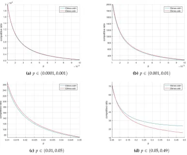
p∈(0.0001, 0.49)with stepsizes of 0.00001 forp. Figure 1 shows that for p∈(0.0723, 0.49)Etimes odd- has a better competitive ratio than Etimes odd+. Atp=0.0723 the competitive ratios are the same for both Etimes odd- and Etimes odd+ and for values ofp<0.0723 Etimes odd+ has a better competitive ratio. This is intuitive, because Etimes odd- needs one more iteration than Etimes odd+ to eventually find the item and whenpgets smaller, the distance travelled in one iteration gets larger, so an extra iteration will cost more. Also the differences between the competitive ratios become smaller whenpis tending to 0.
So, when using Etimes to solve the cow-path problem in the average-case scenario and whenEis odd, Etimes odd+ will be used whenp<0.0723 and otherwise Etimes odd- will be used.
2.3.3 Comparing the algorithms
In this subsection the standard factor algorithm, 4times and Etimes are compared for different probabilities pin the average-case scenario. In the matlabscriptcompetitiveratios.m(Appendix B) the optimal factorsaof the distance function fj=aj−1,∀j≥1,a>1 and the optimal competitive ratios are calculated for the three algorithms. The results are shown in Tables 1 and 2. The probabilities are expressed in the expected value to make a clear distinction between the odd and even cases.
For all algorithms the factor a converges to 1 when p is tending to 0. When p gets smaller the standard factor algorithm and 4times show almost equal values for the factors a and the competitive ratios. The competitive ratios of the odd expected values are slightly higher than those of the even expected values. This is the case, because the probabilities are slightly lower for the odd expected values. Whenptends to 0, these differences seem to become smaller.
(a)p∈(0.0001, 0.001) (b)p∈(0.001, 0.01)
[image:8.612.102.488.92.413.2](c)p∈(0.01, 0.05) (d)p∈(0.05, 0.49)
Figure 1:Optimal competitive ratios for algorithm Etimes when E is odd
factora
E= 1p standard factor algorithm 4times Etimes
E=103+1 1.0010 1.0010 1.0256
E=103 1.0010 1.0010 1.0256
E=102+1 1.0099 1.0099 1.0793
E=102 1.0100 1.0100 1.0796
E=101+1 1.0909 1.0959 1.1731
[image:8.612.97.538.439.548.2]E=101 1.1000 1.1066 1.2397
Table 1:Optimal values of a for the different algorithms and different values of p
Competitive ratios
E= 1p standard factor algorithm 4times Etimes
E=104+1 5.4374791·104 5.4374789·104 2.0499645·104
E=104 5.4367355·104 5.4367353·104 2.0491563·104
E=103+1 5.4457183·103 5.4456966·103 2.1648389·103 E=103 5.4382817·103 5.4382600·103 2.1565804·103
E=102+1 5.5280898·102 5.5259874·102 2.5945787·102
E=102 5.4537239·102 5.4516011·102 2.5063924·102
E=101+1 6.3500776·101 6.1830984·101 4.6805626·101
E=101 5.6062334·101 5.4247666·101 3.7109324·101
[image:8.612.85.543.582.716.2]3.
T
he expected travel distance
The average-case scenario is easy to use, because the seeker will find the item with probability
p=1, after having hit the itemEtimes. In the real world, the seeker will also find the item after hitting it on averageEtimes. However, in the real world the item can in theory never be found. This will give some different results for the expected travel distance.
Consider two scenarios where the seeker searches the item two times, with the item hidden at the same location each time andE=10. First the item is found twice after hitting itE =10 times. Then the same experiment is done again and the item is found for example after hitting the item 8 and 12 times. Now the item is found after hitting itEtims on average in both scenarios, however the distance travelled is different in both scenarios, because the distance gets larger with factora
after each iteration. From this perspective it is better to look at the expected travel distance instead of the average-case scenario.
In this section the average-case scenario will not be considered anymore, but there will be looked at the expected travel distance of the seeker. Since in this case not much is known yet, we will first investigate the competitive ratio of the standard factor algorithm. Later the competitive ratio of 4times will be compared to the competitive ratio of the standard factor algorithm.
To calculate the expected distanceE(D), the following formula is used, since we are dealing with a geometric distribution:
E(D) =
∞
∑
n=1
sn·p(1−p)n−1 (1)
Here,pis the probability of finding the item before hitting it andsn is the total distance travelled when hitting the item for thenthtime. In this section the same definition of the distance function
3.1.
The standard factor algorithm
3.1.1 Competitive ratio factor algorithm
Theorem 3.1. The competitive ratio of the standard factor algorithm for the expected travel distance with a non-optimal seeker is (a−1)(2papa−2 a+1)+2−pp.
Proof. In the worst case, the distancedfrom the origin to the item is fi+e, where fi=ai−1and e>0 is some small number. Then the expected travel distance is:
E(D) =
∞
∑
n=1
sn·p(1−p)n−1
= ∞
∑
n=1 2· i+n∑
j=1fj+ (−1)n+1·d
·p(1−p)n−1
= ∞
∑
n=1 2· i−1+n∑
j=0
aj+ (−1)n+1·d·p(1−p)n−1
= ∞
∑
n=0 2· i+n∑
j=0aj+ (−1)n·d·p(1−p)n
=
∞
∑
n=0
2· a
i+n+1−1
a−1 + (−1)
n·d·p(1−p)n
= 2p a−1 ·
∞
∑
n=0
(ai+n+1−1)(1−p)n+dp·
∑
∞ n=0(−1)n(1−p)n
= 2p a−1 ·
∞
∑
n=0
ai+n+1(1−p)n−
∞
∑
n=0
(1−p)n+dp·
∞
∑
n=0
(−(1−p))n
= 2p a−1 ·
ai+1
∞
∑
n=0
(a(1−p))n− 1 p
+dp· 1
2−p = 2p
a−1 ·
ai+1
pa−a+1− 1
p
+d· p
2−p , |a(1−p)|<1 =ai−1· 2pa
2
(a−1)(pa−a+1)
− 2
a−1+d·
p
2−p ≤d· 2pa
2
(a−1)(pa−a+1)+ p
2−p
So, the competitive ratio for the standard factor algorithm for the expected travel distance, with a non-optimal seeker is (a−1)(pa2pa2−a+1)+2−pp.
3.1.2 Optimizing the standard factor algorithm
The competitive ratio of the standard factor algorithm depend on both aand p, just as in the average-case scenario. Since a can be chosen, we want to find the value for a such that the competitive ratio (a−1)(2papa−2 a+1)+2−pp is minimal.
Theorem 3.2. For the f actor algorithm with a non-optimal seeker and general distance function fj=aj−1 the competitive ratio is minimal when a= 2−2p.
Proof. The functiong(a):= (a−1)(pa2pa−2 a+1)+2−pp needs to be minimized with respect toato obtain an minimal competitive ratio for this algorithm. Firstly, notice only a local minimum in the domaina∈ (1,1−1p)is necessary to improve the competitive ratio. Secondly, the function gis a polynomial function, sogis a differentiable real function. Therefore, the critical point can be found by determining where the derivative ofgis equal to zero:
g0(a) =− 2pa((p−2)a+2) (a−1)2((p−1)a+1)2 =0
This results in a critical point at a = 2−2p, which lies inside the domain 1 < a ≤ 1
1−p, since p∈(0, 1).
Looking at the derivative ofgright before the critical point, we see that it is negative there. Just after the critical point the derivative is positive. The condition that|a(1−p)|=|2pp−−22|<1 also holds, sincep∈(0, 1). Therefore, the functionghas a local minimum ata= 2−2p. So, the standard factor algorithm with a non-optimal seeker and general distance function fj has an minimal competitive ratio whena= 2−2p.
3.1.3 Minimizing the competitive ratio for the standard factor algorithm
Theorem 3.3. For the standard factor algorithm with a non-optimal seeker and general distance function fj=aj−1the minimal competitive ratio is 8p+
p
2−p for the optimal value a= 2−2p.
Proof. If we substitutea= 2−2p in the competitive ratio (a−1)(pa2pa2−a+1)+2−pp, we get the following:
2pa2
(a−1)(pa−a+1) + p
2−p =
2p 2−2p2
( 2−2p
−1)(p 2−2p
− 2
2−p
+1)+ p
2−p
=
8p (2−p)2 4(p−1) (2−p)2 +
2(2−p) (2−p) −1
+ p
2−p
= 8p (2−p)2 4(p−1) (2−p)2 +1
+ p
2−p
=
8p (2−p)2 4(p−1) (2−p)2 +
(2−p)2 (2−p)2
+ p
2−p
= 8p (2−p)2
p2 (2−p)2
+ p
2−p = 8
p + p
Whenp=1, this minimal competitive ratio for the standard factor algorithm is 9 and the optimal valuea=2, so it has the same optimal values as in the deterministic case. When pgets smaller the second term 2−pp tends to 0 and the first term grows to infinity. The value ofatends to 1 forp
tending to zero, just as in the average-case scenario.
3.2.
Algorithm 4times
In the last subsection the competitive ratio is determined and optimized for the standard factor algorithm. The aim is to do the same for 4times, such that both algorithms can be compared again. To determine the competitive ratio for 4times formula 1 from the beginning of this section is used.
sn is a bit harder to define in terms of sums for 4times as was done in the previous subsection for the standard factor algorithm. Forn≥4 this does not give any problems andsn can be written as follows:
sn=2· i+n−2
∑
j=1
(2fj−fj−2) + (−1)n+1·d (2)
Forn = 1, 2, 3 the distances can be written such that formula 2 is valid forn ≥ 1, but some additional terms must be added, because the first four times the seeker hits the item, it hits the item travelling a relative small distance compared to the iterations afterwards.s1,s2ands3are
defined as following:
s1=2·
i+n−2
∑
j=1
(2fj−fj−2) + (−1)n+1·d+2·(2fi+1+2fi− fi−1−fi−2)
s2=2·
i+n−2
∑
j=1
(2fj−fj−2) + (−1)n+1·d+2·(fi+2+2fi+1−fi−1)
s3=2·
i+n−2
∑
j=1
(2fj−fj−2) + (−1)n+1·d+2·(fi+2−fi)
To calculateE(D),sn is splitted fors1,s2ands3. Here the additional terms fors1,s2ands3must
be multiplied byp,p(1−p)and p(1−p)2respectively. For convenience, this part ofE(D)will be
defined asR, when calculating the competitive ratio for the algorithm.
R=2·(p(2fi+1+2fi− fi−1−fi−2) +p(1−p)(fi+2+2fi+1−fi−1) +p(1−p)2(fi+2−fi)) =p(4ai+1+8ai+2ai−1−4ai−2−2ai−3)−p2(6ai+1+4ai−4ai−1−2ai−2) +p3(2ai+1−2ai−1) =2ai−1 a2(p3−3p2+2p) +a(−2p2+4p) + (−p3+2p2+p) +a−1(p2−2p)−a−2p
3.2.1 Competitive ratio 4times
Theorem 3.4. The competitive ratio of 4times for the expected travel distance with a non-optimal seeker is
4p−2ap2
(a−1) (ap−a+1)+ p
2−p +2·(0.3849a
2+2a+2).
Proof. In the worst case, the distancedfrom the origin to the item is fi+e, where fi=ai−1and e>0 is some small number. Then the expected travel distance is:
E(D) =
∞
∑
n=1
sn·p(1−p)n−1
= ∞
∑
n=1 2· i+n−2∑
j=1
(2fj−fj−2) + (−1)n+1·d
·p(1−p)n−1+R
= ∞
∑
n=1 2· i+n−3∑
j=0
(2aj−aj−2) + (−1)n+1·d·p(1−p)n−1+R
=
∞
∑
n=1
4·a
i+n−2−1 a−1 −2·
ai+n−4−1
a−1 + (−1)
n+1·d·p(1−p)n−1+R
=
∞
∑
n=1
4ai+n−2−2ai+n−4−2
a−1 + (−1) n+1·d
·p(1−p)n−1+R
=
∞
∑
n=0
4ai+n−1−2ai+n−3−2
a−1 + (−1)
n·d·p(1−p)n+R
= 2p a−1·
∞
∑
n=0
(2ai+n−1−ai+n−3−1)(1−p)n+dp·
∑
∞ n=0(−1)n(1−p)n+R
= 2p a−1·
∞
∑
n=0
2ai+n−1(1−p)n−
∞
∑
n=0
ai+n−3(1−p)n−
∞
∑
n=0
(1−p)n+dp·
∞
∑
n=0
(−(1−p))n+R
= 2p a−1·
2ai−1
∞
∑
n=0
(a(1−p))n−ai−3
∞
∑
n=0
(a(1−p))n−1 p
+dp· 1
2−p +R = 2p
a−1·
2ai−1−ai−3
pa−a+1 − 1
p
+d· p
2−p +R , |a(1−p)|<1 =ai−1· 4p−2pa
−2
(a−1)(pa−a+1)
− 2
a−1 +d·
p
2−p+R ≤d· 4p−2pa
−2
(a−1)(pa−a+1)+ p
2−p
+R
≤d· 4p−2pa
−2
(a−1)(pa−a+1)+ p
2−p+
2· a2(p3−3p2+2p) +a(−2p2+4p) + (−p3+2p2+p) +a−1(p2−2p)−a−2p
≤d· 4p−2pa
−2
(a−1)(pa−a+1)+ p
2−p +2·(0.3849a
So, the competitive ratio for 4times for the expected travel distance, with a non-optimal seeker
is 4p−
2p a2
(a−1) (ap−a+1)+ p
2−p +2·(0.3849a
2+2a+2).
3.3.
Comparing the standard factor algorithm and 4times
For the standard factor algorithm it is known that the optimal value ofais equal to 2−2p and that the minimal competitive ratio is 8p+2−pp. For the competitive ratio of 4times determined in the last subsection, it is harder to find the optimal value foraand hereby also the minimal competitive ratio. Therefore the optimal value ofais determined by only optimizingafor 4p−
2p a2 (a−1) (ap−a+1),
assuming thatawill tend to 1 for smallp, 2(0.3849a2+2a+2)depending onawill not affect the competitive ratio too much.
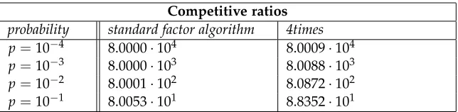
This strategy seems to work quite good. As an example we takep=0.1. The difference between the minimal competitive ratio and the competitive ratio determined in the way stated in the last paragraph is only of the order of 10−4, while these competitive ratios are of the order 102. In Tables 3 and 4 the values ofaand the competitive ratios are shown for the standard factor algorithm and 4times for different values ofp. The value ofafor 4times is tending to the same value as for the optimal value ofafor the standard factor algorithm and hereby tends to go to 2−2p as well for smallp.
Just as for the average-case scenario, the differences between the competitive ratio of these algorithms get smaller forptending to 0. Only now the standard factor algorithm has a better competitive ratio than 4times. The values ofaand the competitive ratios in Tables 3 and 4 are calculated in the matlabscriptcompetitiveratios2.m(Appendix C).
factora
probability standard factor algorithm 4times
p=10−4 1.000050003 1.000050003
p=10−3 1.000500250 1.000500251
p=10−2 1.005025126 1.005025627
[image:14.612.146.468.449.529.2]p=10−1 1.052631579 1.053154469
Table 3:optimal values of a for the different algorithms for different values of p
Competitive ratios
probability standard factor algorithm 4times p=10−4 8.0000·104 8.0009·104
p=10−3 8.0000·103 8.0088·103
p=10−2 8.0001·102 8.0872·102
p=10−1 8.0053·101 8.8352·101
Table 4:Optimal competitive ratios for the different algorithms for different values of p
[image:14.612.146.468.581.660.2]3.4.
Simulation of the standard factor algorithm
Now the theoretical competitive ratios for the cow-path problem with a non-optimal seeker are determined for the standard factor algorithm and 4times. To see how tight these bounds are, the problem has been simulated in the matlabscriptcowpath.m(Appendix D). The seeker searches with the same probability for 100.000 times and the item is hidden at the same place each time. The standard factor algorithm is used to solve the cow-path problem, because until now this is the best algorithm and the easiest algorithm to implement.
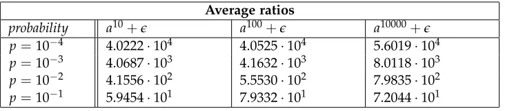
In Table 5 the average ratios are shown. Theaverage ratiois the total distance travelled divided by the number of searches and this value divided bydthe distance to the item.
For smaller values of pthe ratios are relatively smaller compared to the calculated competitive ratios in most cases. This is because when p is smaller a = 2−2p is automatically also smaller. This means that the item is lying closer to the origin, which means that it is easier to find. This is also the reason why fora10000+ethe average ratio for p= 10−4 is smaller compared to the calculated competitive ratios than the average ratios for the other probabilities, because in this case the item is still only hidden around 150 in distance from the origin. For all values ofp, the average ratio grows when the item is hidden further away from the origin. In one case the average ratio even exceeds the competitive ratio. This is because the competitive ratios are determined for the expected distance. When the seeker would do more searches the average ratio would converge to this expected value which must be less or equal to the competitive ratio.
Average ratios
probability a10+e a100+e a10000+e
p=10−4 4.0222·104 4.0525·104 5.6019·104
p=10−3 4.0687·103 4.1632·103 8.0118·103
p=10−2 4.1556·102 5.5530·102 7.9835·102
[image:15.612.125.491.348.429.2]p=10−1 5.9454·101 7.9332·101 7.2044·101
4.
C
onclusion
This paper started with looking at the average-case scenario for the cow-path problem with a non-optimal seeker. Two new algorithms were introduced and show better competitive ratios than the ratio of the known standard factor algorithm. Etimes is by far the best algorithm for the average-case scenario, with a competitive ratio converging to 2p forptending to 0. The standard factor algorithm and 4times seem to find the item in equal time whenpis tending to 0, with both a competitive ratio of around 5.4366p . This means that for ptending to 0, the search distance is tending to infinity for all discussed algorithms.
The average-case scenario was investigated to get some feeling for the cow-path problem with a non-optimal seeker, but it shows only a few similarities compared to the expected travel distance. In both cases we do see that the factoraof the distance function f converges to 1 and that the competitive ratios grow to infinity forptending to 0. An intuitive explanation foratending to 1 whenptends to 0 would be that if pgets smaller the item would be harder to find, so the seeker does not want to take the risk of travelling far away when already searching on the interval of where the item is hidden.
However, the average-case scenario is not the same as the real situation, where we look at the expected travel distances for the algorithms. It is more interesting to do more research for the expected travel distance only, since the average-case scenario is a scenario which will less likely be used.
For the expected travel distance, investigated in the second part of this paper, 4times performs worse than the standard factor algorithm. It might still be interesting to look at the competitive ratio for Etimes, but it is impossible to find this ratio in the same way as for the standard factor algorithm and 4times, because then additional terms have to be taken into account fors1untilsE−1
whereEcan be infinitely large. A competitve ratio might be found by looking at the algorithm
E-periodically.
For the standard factor algorithm we found an elegant competitive ratio of 8p+2−pp which is exactly 9 for p =1 just as the competitive ratio for cow-path problem without a non-optimal seeker. For p tending to 0 this ratio goes to 8p which is a higher ratio than the ratios for the algorithms in the average-case scenario. In the simulations the differences between the competitive ratio of 8p+2−pp and the simulated average ratio get smaller when the item is hidden further away. For the items were hidden relatively close to the origin we even found average ratios better than the competitive ratio of the average-case scenario for the standard factor algorithm. Therefore, it might be interesting to look at upper bounds for the cow-path problem depending on where the item is hidden.
Since 4times performs worse than the standard factor algorithm and the competitive ratio grows linearly forptending to 0, there might not be a better algorithm than the standard factor algorithm for this problem. This research contradicts the intuitive claim made in the introduction, that it seems that for ptending to 0 there must be better algorithms seeking more often further away from the origin. Therefore, it is interesting for further research to investigate whether the standard factor algorithm is an optimal algorithm for the cow-path problem using a non-optimal seeker. Besides this, many other things can be investigated for further research. In this paper there is only looked at the worst case ratio. Algorithms might perform differently looking at lower bounds for example or finding the item in only a certain percentage of the cases. It is also interesting to see how the non-optimal seeker influences thew-lane cow-path problem whenw6=2.
R
eferences
Baeza-Yates, R. A., Culberson, J. C. & Rawlins, G. J. E. (1993), ‘Searching in the Plane’,Information and Computation106(2), 234–252.
URL:http://www.sciencedirect.com/science/article/pii/S0890540183710540
Beck, A. (1964), ‘On the linear search problem’,Israel Journal of Mathematics2(4), 221–228.
Beck, A. & Newman, D. J. (1970), ‘Yet more on the linear search problem’, Israel Journal of Mathematics8(4), 419.
Bellman, R. (1963), ‘Problem 63-9, an optimal search’,Siam Review5(3), 274.
Demaine, E. D., Fekete, S. P. & Gal, S. (2006), ‘Online searching with turn cost’,Theoretical Computer Science361(2-3), 342–355.
Franck, W. (1965), ‘An Optimal Search Problem’,Siam Review7(4), 503–512.
Fuchs, B., Hochstättler, W. & Kern, W. (2003), ‘Online Matching On a Line’,Electronic Notes in Discrete Mathematics13(1), 49–51.
Gal, S. (1974), ‘Minimax Solutions for Linear Search Problems’,SIAM Journal on Applied Mathematics
27(1), 17–30.
Heukers, F. (2017), Searching with Imperfect Information, Technical report, University of Twente.
Jez, A. & Łopusza ´nski, J. (2009), ‘On the two-dimensional cow search problem’, Information Processing Letters109(11), 543–547.
Kao, M. Y., Reif, J. H. & Tate, S. R. (1996), ‘Searching in an Unknown Environment: An Optimal Randomized Algorithm for the Cow-Path Problem’,Information and Computation131(1), 63–79. Spieser, K. & Frazzoli, E. (2012), The Cow-Path Game: A competitive vehicle routing problem,in
A.
solve
_
cubic
.
m
1 %SOLVE_CUBIC solves the real root of g'(a) for Etimes odd+/-, which is 2 %greater than 1 for each p element of the interval (0.0001,0.49), to 3 %obtain the optimal competitive ratio. This root is then substituted into 4 %the competitive ratios, which are plotted on different intervals for 5 %Etimes odd+ and Etimes odd-.
6
7 clear all
8 k=1; 9 l=1;
10 y= zeros(1,48991); %preallocation arrays of optimal a's 11 z= zeros(1,48991);
12 y2= zeros(1,48991); %preallocation arrays of optimal competitive ratios 13 z2= zeros(1,48991);
14
15 %Calculating optimal a's and competitive ratios for Etimes odd+ 16 for p= 0.0001:0.00001:0.49
17 a=2*p-2;
18 b=3-5*p;
19 c=4*p; 20 d=-1+p;
21 x = roots([a b c d]);
22 y(k)=x(imag(x)==0 & real(x)>1); %array of roots for each p
23 y2(k)= (((1/p)+1)*y(k)^3-((1/p)-1)*y(k))/(y(k)-1)+2*y(k)^2+1; %array of ... competitive ratios for each p
24 k=k+1;
25 end 26
27 %Calculating optimal a's and competitive ratios for Etimes odd-28 for p= 0.0001:0.00001:0.49
29 a=3*p-3; 30 b=4-4*p;
31 c=1-3*p;
32 d=6*p-2;
33 x = roots([a b c d]);
34 z(l)=x(imag(x)==0 & real(x)>1); %array of roots for each p
35 z2(l) = (((1/p)-1)*z(l)^4-((1/p)-3)*z(l)^2)/(z(l)-1)+1; %array of competitive ... ratios for each p
36 l=l+1;
37 end 38
39 g= 0.0001:0.00001:0.49; %defining x-values plot 40
41 %making four plots on different intervals to compare Etimes odd+ and Etimes odd-42 figure
43 hold on
44 grid on
45 xlabel('p')
46 ylabel('competitive ratio')
47 axis([0.0001 0.001 2000 20000])
48 plot(g,y2)
49 plot(g,z2,'r')
50 legend('Etimes odd+', 'Etimes odd-')
51 hold off
52
53 figure
54 hold on
55 grid on
56 xlabel('p')
57 ylabel('competitive ratio')
58 axis([0.001 0.01 250 2000])
59 plot(g,y2)
60 plot(g,z2,'r')
61 legend('Etimes odd+', 'Etimes odd-')
62 hold off
63
64 figure
65 hold on
66 grid on
67 xlabel('p')
68 ylabel('competitive ratio')
69 axis([0.01 0.05 70 270])
70 plot(g,y2)
71 plot(g,z2,'r')
72 legend('Etimes odd+', 'Etimes odd-')
73 hold off
74
75 figure
76 hold on
77 grid on 78 xlabel('p')
79 ylabel('competitive ratio')
80 axis([0.05 0.5 10 75])
81 plot(g,y2)
82 plot(g,z2,'r')
83 legend('Etimes odd+', 'Etimes odd-')
B.
competitiveratios
.
m
1 %COMPETITIVERATIOS calculates the different optimal values of a and the 2 %different optimal competitive ratios for the standard factor algorithm, 3 %4times and Etimes for a given value of p in the average-case scenario. 4
5 clear all
6 format long
7 p= 1/100000001; %probability finding the item 8
9 %competitive ratio for standard factor algorithm
10 standardfactor = (2*(1+p)^(1/p+1))/(p)+ (-1)^(1/p+1) %competitive ratio 11 aF = 1+p %optimal factor for standard factor algorithm
12
13 %competitive ratio for 4times 14 a=4*p-2;
15 b=2-2*p;
16 c=1-4*p;
17 d=3*p-1;
18 x4= roots([a b c d]);
19 a4=x4(imag(x4)==0 & real(x4)>1) %optimal value of a
20 times4 = (4*a4^(1/p-1)-2*a4^(1/p-3))/(a4-1)+(-1)^(1/p+1) %competitive ratio 21
22 %competitive ratio for Etimes
23 if rem((1/p),2)==0 %depending on whether E is even or odd
24 a=2;
25 b=-3;
26 c=0;
27 d=-2*p+1;
28 xE= roots([a b c d]);
29 aE=xE(imag(xE)==0 & real(xE)>1) %optimal value of a
30 Etimes = ((1/p)*aE^3-(1/p)*aE+2*aE)/(aE-1)-1 %competitive ratio 31 elseif p<0.0723
32 a=2*p-2;
33 b=3-5*p;
34 c=4*p;
35 d=-1+p;
36 x = roots([a b c d]);
37 aE=x(imag(x)==0 & real(x)>1) %optimal value of a
38 Etimes= (((1/p)+1)*aE^3-((1/p)-1)*aE)/(aE-1)+2*aE^2+1 %competitive ratios for ... each p
39 else
40 a=3*p-3;
41 b=4-4*p;
42 c=1-3*p;
43 d=6*p-2;
44 x = roots([a b c d]);
45 aE=x(imag(x)==0 & real(x)>1) %optimal value of a
46 Etimes = (((1/p)-1)*aE^4-((1/p)-3)*aE^2)/(aE-1)+1 %competitive ratio 47 end
C.
competitiveratios
2.
m
1 %COMPETITIVERATIOS2 calculates the different optimal values of a and the 2 %different optimal competitive ratios for the standard factor algorithm 3 %and 4times for a given value of p for the expected travel distance. 4
5 clear all
6 format long
7 p= 0.0001; %probability finding the item 8
9 %competitive ratio for standard factor algorithm 10 standardfactor = 8/p + p/(2-p); %competitive ratio 11 aF = 2/(2-p);
12
13 %competitive ratio for 4times 14 a=4*p-4;
15 b=4-2*p;
16 c=4-4*p;
17 d=3*p-6;
18 e=2;
19 x4= roots([a b c d e]);
20 a4=x4(imag(x4)==0 & real(x4)>1) %optimal value of a
21 %%times4 = (4*p-(2*p)/a4^2)/((a4-1)*(a4*p-a4+1))+2*(a4^2*(2*p^3+5*p^2+3*p) 22 %-p^3+a4*(2*p^2+4)-2*p^2+(-p^2-2*p)/a4-p/a4^2+p)+p/(2-p); %lower bound 23 times4 = ((4*p-(2*p)/a4^2)/((a4-1)*(a4*p-a4+1)))+0.7698*a4^2+4*a4+4+(p/(2-p))
D.
cowpath
.
m
1 %COWPATH solves the cow-path problem with a non-optimal seeker using the 2 %standard factor algorithm with optimal a. It lets the seeker search N 3 %times for the item hidden at the same position and calculates the average 4 %distance travelled. The average ratio is then determined by dividing the 5 %average distance by d
6
7 clear all 8 format long
9
10 n=0; %initialization for i, j, n, avgdistance and avgj 11 i=1;
12 j=1;
13 avgdistance = 0;
14 avgj = 0;
15 p= 0.1; %probability seeker finds object
16 a= 2/(2-p); %factor of distance, element of the interval (1,2) 17 x= a^10000+0.0001; %place object is hiding
18 N = 100000; %number of searchings 19 %js = zeros(N, 1); %initialization 20
21
22 %finding a^n, so when the seeker will first hits the object 23 while a^n< abs(x)
24 n=n+1;
25 end 26
27 if x<0 & rem(n,2)==1 | x>0 & rem(n,2)==0
28 n=n-1; 29 else
30 n=n;
31 end 32
33 for i= 1:N %number of searchings
34 while rand(1)>p %j is number of times not finding the object,...
35 %when hitting it
36 j=j+1;
37 end
38
39 if rem(j,2)==0 %determining the travelled distance, depending on if...
40 %j is even or odd
41 distance = 2*((a^(n+j)-1)/(a-1))-abs(x);
42 else
43 distance = 2*((a^(n+j)-1)/(a-1))+abs(x);
44 end
45
46 avgdistance = ((i-1)*avgdistance+distance)/i; %determining the ...
47 %average distance
48 %js(i) = j; %vector with all values for j 49 j=1; %setting back value for j
50 end 51 52
53 avgdistance;
54 compratio = avgdistance/x %average ratio from simulation 55 standardfactor = 8/p + p/(2-p) %theoretic ratio