Interfaces of topological insulators and superconductors

(1)

䄀甀最甀猀琀

㄀　Ⰰ

㈀　㄀㠀

䴀愀猀琀攀爀ᤠ

猀

吀栀攀猀椀

猀

䄀瀀瀀氀

椀

攀搀

倀栀礀猀椀

挀猀

☀

䄀瀀瀀氀

椀

攀搀

䴀愀琀栀攀洀愀琀椀

挀猀

䤀渀琀

攀爀昀愀

挀攀猀

漀昀

琀漀瀀

漀氀漀

最椀挀

愀氀椀

渀猀甀

氀愀琀漀

爀猀愀

渀搀

猀甀瀀

攀爀挀

漀渀搀

甀挀琀

漀爀猀

䰀椀渀

搀攀

䄀⸀䈀

⸀ 伀

氀搀攀

伀氀琀

栀漀昀

䜀爀愀搀甀愀琀椀

漀渀挀漀洀洀椀

琀琀攀攀

䄀瀀瀀氀

椀

攀搀倀栀礀猀椀

挀猀

倀爀漀昀

⸀

搀爀⸀

䄀⸀

䈀爀椀

渀欀洀愀渀

䐀爀⸀

䜀⸀

䠀⸀

䰀⸀

䄀⸀

䈀爀漀挀欀猀

䐀爀⸀

䌀⸀

䰀椀

䈀⸀

搀攀

刀漀渀搀攀Ⰰ

䴀⸀

匀挀⸀

䄀瀀瀀氀

椀

攀搀䴀愀琀栀攀洀愀琀椀

挀猀

䄀瀀瀀氀

椀

攀搀䴀愀琀栀攀洀愀琀椀

挀猀

(2)

Abstract

At every interface with a superconductor, there is a probability that an incident electron is reflected as a spin-flipped hole, which is known as Andreev reflection. In certain geometries consisting of a topological insulator and ans-wave superconductor, Andreev reflection can lead to the formation of a Majorana bound state (MBS). Since a MBS obeys non-Abelian statistics, it can serve as a build-ing block for topological quantum bits in future devices. In this thesis, we investigate interfaces of topological insulators and superconductors, both theoretically and experimentally.

The transport through topological Josephson junctions has a sub-harmonic gap structure as a result of multiple Andreev reflections. Oscillations in the current occur when an electron can overcome the energy gap after performingn−1 Andreev reflections. We show that in a two dimensional topo-logical Josephson junction, this energy gap depends on the Fermi surface mismatch between the superconductor and the topological insulator. This implies that the full spectrum shifts according to the mismatch, although this is hardly visible after angle averaging the current. Furthermore, we show that in the absence of an applied voltage, a bound state can exist with the same energy as seen in chiralp-wave superconductors.

(3)

(4)

a

Introduction

Our technology is quickly developing, but our conventional transistor-based computers cannot keep up. The operating frequency of our computers is restricted, they dissipate large amounts of heat and the limit of downscaling the physical size is almost reached. We are in need of a new technology that can outperform the conventional computer in terms of operating frequency. A promising candidate is the so-called quantum computer.

a A conventional, transistor-based computer uses bits that can only represent the values 0 and 1. It returns 0 if the transistor is “off” and 1 if it is “on”. A quantum computer utilizes the quantum properties of superposition, which means that a quantum bit (qubit) can be in both states at the same time. It adapts the values 0 and 1 simultaneously and therefore, it is twice as fast. Two qubits hold four values at once: 00, 01, 10 and 11. The number of values as a function of the number of bits in a conventional computer scales asn, while in a quantum computer, it scales as 2n_{, implying}

that it is exponentially faster. Only 20 qubits are needed to take over a million values. [1, 2]

a The idea of the quantum computer was initially proposed by Richard Feynman in 1981. He stated that accurate and efficient simulation of a quantum mechanical system is impossible on a conventional computer. They cannot handle the complexity and the exponentially growing amount of data that is inherent to quantum systems. A quantum computer, on the other hand, “is built of quantum mechanical elements which obey quantum mechanical laws” and should therefore be able to do the job. [3] Besides being used for fundamental quantum physics simulations, other applications are in, e.g., information theory, engineering of molecules, cryptography and language theory. [4] Moreover, the quantum computer will most likely have an even bigger impact than we can imagine. The conventional computer was first built solely to simulate Newtonian mechanics. In the 1950s, people could not imagine why anyone would want a computer in their home. A quantum computing expert at MIT claims that replacing our conventional computers with quantum computers will have the same huge impact as the conventional computer originally had; it is going to be a milestone in technology. [5]

a At the moment, quantum computers have been realised at a proof of concept scale, but there are still many challenges to overcome. [6] One of the greatest challenges is protecting the qubits from noise from the surroundings that perturb the quantum states. [4] Current quantum computers can hold their quantum states for only a fraction of a second before becoming too seriously perturbed. IBM’s 50 qubit computer that was built in 2017 is able to hold a quantum state for only 90 microseconds. [7]

(9)

[image:9.595.208.369.113.212.2]

2 Introduction

Figure 1: The order of interchanging results in a different state, such that the final states ofAandB are different. From [9].

The quantum state is obtained by the process of interchanging MBSs, which is not very likely to happen as a result of noise. Therefore, a quantum computer based on MBSs is more robust against environmental noise. [8]

a This concept is very appealing, but a lot of work still has to be done. MBSs and their non-Abelian statistics are exotic phenomena and not easy to realise. In order to obtain them, a very specific symmetry of the materials is required. It turns out that this can, for example, be realised by bringing a superconductor into contact with a topological insulator. The goal of this thesis is to investigate the existence of MBSs in systems of topological insulators and superconductors, both theoretically and experimentally.

(10)

a

A note on notation

The use of symbols in mathematics and physics is not always consistent. Two symbols that have very different meanings in both fields are ∆ and∗. Therefore, we will introduce them here separately, to avoid any confusion.

In physics, the Laplacian, or Laplace-operator, is usually denoted by∇2_{. What is actually meant} here is∇2₌_∇·∇_{. In mathematical textbooks, the Laplacian is often denoted by the symbol ∆. This} is very confusing for physicists, since in physics, ∆ corresponds to a property of superconductors. In literature, it is referred to as the energy gap, pair potential or superconducting order parameter, just to name a few.

Another point of confusion is the notation used to describe transpose and conjugate matrices. The symbol ∗ has a different meaning, depending on if we are reading a text on quantum mechanics (physics) or on linear algebra (mathematics). An overview of the notation:

Physics Mathematics

Matrix A A

a11 a12

a21 a22

Transpose matrix AT AT or A0

a11 a21

a12 a22

Conjugate matrix A∗ A¯

a∗11 a∗12

a∗21 a∗22

Conjugate transpose A† A∗

a∗

11 a∗21

a∗ 12 a∗22

(11)

(12)

1

a

Introducing physical concepts

1.1 Quantum mechanics

1.1.1 Classical mechanics vs. Quantum mechanics

Classical mechanics consists mostly of the physics prior to the 20th_{century. It accurately describes} most “normal” systems; systems that are a “normal” size (larger than a molecule and smaller than a planet) and are moving at a “normal” speed (significantly less than the speed of light). [10] Only when one of these “normal” parameters is violated, a different theory is needed.

Quantum mechanics gradually arose to explain experiments that did not match the classical de-scriptions anymore. A famous example is the “ultraviolet catastrophe”, i.e. in classical mechanics, black bodies can emit an infinite amount of energy. [11] This was solved by Planck’s law in 1900 and Einstein’s 1905 paper on the photoelectric effect (explaining the correspondence between energy and frequency) [12]. A couple of years later, in 1927, the famous double slit experiment took place, in which a coherent light source (e.g. a laser) is emitted towards two slits. The resulting interference pattern behind the slits revealed that the light splits into two waves and then combines again, just like a wave would do. This gave rise to the particle-wave duality of light. [13] In the mid-1920s, Schr¨odinger, Heisenberg and Born developed the mathematical formalisms, which we know today as quantum mechanics. [14] It describes nature on the energy smallest scales of energy levels and considers subatomic particles.

There are three major differences in which quantum mechanics differs from classical mechanics. First of all, since quantum mechanics considers small scales and individual particles, the energy, momentum and other quantities of a system may be restricted to discrete values. This is called “quantization” and is what quantum mechanics is named after. Secondly, objects have characteris-tics of both particles and waves (particle-wave duality). Thirdly, classical mechanics assumes that an object has definite, knowable attributes, such as its position and momentum. In quantum me-chanics on the other hand, there can be limits to the precision with which quantities can be known (uncertainty principle). [14]

(13)

6 CHAPTER 1. INTRODUCING PHYSICAL CONCEPTS

denoted byψ(x). The wave function can be interpreted as a complex-valued probability amplitude. More concretely, [14]

Z b

a

|ψ(x)|2_dx_{= probability of finding the particle between}_a_and_b.

The wave function can be obtained via the Schr¨odinger equation; the most famous equation of quantum mechanics. The time-independent Schr¨odinger equation is an eigenvalue equation that is known as

Hψ=Eψ, (1.1)

whereHis the Hamiltonian, which is mathematical representation of the physical phenomena in the system. The wave functionψis the eigenfunction of the Hamiltonian. The eigenvalueEcorresponds to the energy of the system. We will see that the Hamiltonian is a function of momentumk, which makes the energy momentum dependent as well, i.e. E =E(k). The relation between E and kis called the dispersion relation.

a The Schr¨odinger equation is just an example. In fact, all observables in quantum physics can be written as the real eigenvalues of Hermitian operators. [14]

1.1.2 Electrons and holes

In particle physics, every particle has a corresponding antiparticle. The antiparticle has the same mass, but has the opposite charge. We will focus on electrons (the particles). In solid state physics, the antiparticle of an electron is called a hole (a positron in particle physics). The electron charge is defined as−e, such that a hole has charge +e.

A hole is usually considered as a missing electron. This can be interpreted by second quantization operators. The creation operator ˆc†_k creates a particle in quantum statek, whereas the annihilation operator ˆck removes it (or, equivalently, creates the corresponding antiparticle). Since a hole is a

missing electron, the creation of a hole the same is as the annihilation of an electron.

The final property of electrons and holes we will discuss here is their dispersion relation. The notion of treating a hole as a missing electron turns out to be very important here. In the sim-plest case of a normal metal (a metal which does not have any special properties), the Schr¨odinger equation for electrons in one dimension is given by [14]

Hψ=

−~

2

2m ∂2 ∂x2 −µ

ψ=Eψ, (1.2)

where the first term describes the kinetic energy, with~the reduced Planck constant andmis the

mass. The second term, µ, is the chemical potential, which can be considered as just a constant offset to the energy. Assuming a simple propagating wave, i.e. ψ(x) =eikx_{, we find that the energy}

(and therefore, the dispersion relation) is given by

E= ~ 2_k2

2m +µ. (1.3)

We can do the same for holes in which case we find the same result with a minus sign (this will be explained in more detail further on). Hence, we have two parabolic dispersionsE ∼ ±k2. The Fermi levelEF is the energy level of interest. For convenience, we takeEF =µ(which we can do

(14)

1.1. QUANTUM MECHANICS 7

electron as a solid circle and a hole as a open circle. The arrows connected to these circles represent the direction of the group velocity.

In the simple case we have considered so far, it then follows that the wave function of the particle and antiparticle are related by complex conjugation. For example, consider a propagating electron described by ψ(x) = eikx_{. The corresponding hole has the wave function} _ψ∗₍_x_{) =} _e−ikx_{. This}

property is known as “time-reversal symmetry” and will play an important role throughout this work. Note that in many cases time-reversal symmetry is broken, most notably, by a magnetic field.

E

k

[image:14.595.291.484.240.339.2]

EF

Figure 1.1: Parabolic dispersion.

electron hole particle anti-particle

charge −e +e

creation ˆc†_k cˆk

annihilation ˆck cˆ†_k

energy E −E

momentum k −k

wave function ψ ψ∗

Table 1.1: Properties of electrons and holes.

In order not to get confused, note that we have two ways of considering electrons in a system: the “ordinary picture” and the “particle-hole picture”. Recall that the states up to the Fermi level are filled. This is called the ground state. In the ordinary picture we are concerned with these electrons. Exciting an electron leaves an empty state behind. In the particle-hole picture, we do not consider the electrons up to the Fermi level. This has the consequence that exciting electrons requires us to consider missing electrons, i.e. holes. The ordinary picture and particle-hole picture are sketched in Fig. 1.2. Throughout the rest of this work, we will mainly focus on the particle-hole picture.

Figure 1.2: Two ways of considering non-interacting Fermi systems. Image from [15].

1.1.3 Bosons, fermions, anyons

Suppose we have two particles. In the simple case of classical mechanics, we could say that particle 1 is in state ψa(x) and particle 2 is in stateψb(x). In that case, the total wave function would be

simply given by [14]

(15)

This assumes that we can tell the particles apart, otherwise it would not make any sense to give the particles number 1 and 2. In quantum mechanics, this is not the case. Particles are indistinguishable and we have to take this into account in the wave function. Two possible ways to do so are

ψ±(x1, x2) = 1

√

2[ψa(x1)ψb(x2)±ψb(x1)ψa(x2)], (1.5) where 1/√2 is just a normalization factor. [14] These two ways describe two kinds of particles:

bosons (corresponding to the + sign) and fermions (the − sign). Some examples: photons are

bosons, electrons are fermions. [14]

An important concept related to this topic isspin. Particles carry two types of angular momentum: orbital angular momentum and spin angular momentum (or, in short, spin). Spin is quantized and can either have integer or half-integer values. It turns out that all particles with integer spin are bosons, while all particles with half-integer spin are fermions. [14] In non-relativistic quantum mechanics, this is taken as an axiom. It follows naturally from the unification of quantum mechanics and special relativity, [16, 17] but this goes beyond the scope of this work. It turns out that there is a connection between the spin and statistics of bosons and fermions. This becomes evident when we try to put two particles in the same state, i.e. ψa=ψb. For bosons, this is not a problem at all.

In the case of fermions, however, the full wave function becomes zero, which means that this is not possible. This is known as thePauli exclusion principle; two identical fermions cannot occupy the same state. [14]

More generally, the wave functions (1.5) have different symmetries. Interchanging two particles (i.e.

x1→x2,x2→x1), we find

bosons ψ(x1, x2) =ψ(x2, x1), fermions ψ(x1, x2) =−ψ(x2, x1),

or in words, the wave function for bosons is symmetric, while the fermion wave function is anti-symmetric. [14] There is, however, one other option:

ψ(x1, x2) =eiφψ(x2, x1), (1.6)

where i =√−1 and φ∈ R is a phase. This type of particle is called an anyon. Note that since

the probability is related to|ψ|2_{, these different types of symmetry are not observable. However, it} turns out to be very relevant, as will be elaborated on in Section 1.4.1.

1.2 Superconductors

Superconductivity has been a hot topic (or perhaps “a cold topic” is more appropriate in this case) since its discovery in 1911. In the early years, only the macroscopic phenomena were known. The basic concept of superconductors is explained in Section 1.2.1.

a Only 46 years later, in 1957, a microscopic theory on superconductivity was postulated by Bardeen, Cooper and Schrieffer.[18] Their theory is now known as theBCS theory(named after the three of them). They received the Nobel Prize in 1972 for their theory. We will briefly touch upon some of the key concepts of their theory in Section 1.2.2.

(16)

1.2. SUPERCONDUCTORS 9

1.2.1 Macroscopic view

A superconductor is a special type of material that has two phases: a superconducting state and a normal state. In order to become superconducting, two properties have to be fulfilled. Firstly, when a superconductor is cooled down below its critical temperature Tc, the electric resistance

suddenly drops to zero. This was discovered by H. Kammerlingh Onnes in 1911, who showed that if mercury is cooled below 4.1 K, it loses all electrical resistance. [21] The lack of electrical resistance allows an electric current flowing through a loop of superconducting wire to last indefinitely. [22] Secondly, a superconductor has a characteristic way of behaving in a magnetic field. [23] There are two types of superconductors. A type I superconductor has a single critical field Hc. If the

applied magnetic field is lower than Hc and the temperature is lower thanTc, the superconductor

excludes the magnetic field, which is called the Meissner effect. [23] A type II superconductor has two critical fields Hc1 and Hc2. In between them, the magnetic field can partially penetrate the superconductor in the form of vortices. BelowHc1, the type II superconductor behaves the same as a type I superconductor. [22] If the temperature is aboveTcor if the applied magnetic field is higher

than Hc (type I) orHc2 (type II), the superconductor behaves like a normal metal. Considering both the critical temperature Tc and the critical field(s), Hc for type I and Hc1, Hc2 for type II, we can construct a phase diagram for the superconductor, as shown in Fig. 1.3. The property of

Superconducting state

Normal state

H Hc

T Tc

(a) Type I

Meissner state

Normal state

H

Hc2

T

Tc

Vortices

Hc1

(b)Type II

Figure 1.3: Phase diagrams of superconductors.

indefinite current and zero resistance makes superconductors very appealing candidates for future electronics, which is why its an interesting type of materials to study. However, the goal of this work is not to look into the details of possibilities for new electronics. We are much more interested in the microscopic phenomena that are going on in superconductors.

1.2.2 Microscopic view

(17)

[image:17.595.100.239.107.320.2]

Table 1.2: Examples of phase transitions from a normal state to a condensed state. From [15].

Figure 1.4: Schematic diagram of a Cooper pair; a pair of electrons with opposite momen-tum (+k and−k) and opposite spin (↑and ↓). The axeskxandkydenote 2D momentum space. The Fermi surface represents the 2D equivalent of the Fermi level EF. Inside, states are filled. The Cooper pair is located just above the Fermi level. Image from [24].

Cooper pairs are pairs of electrons, but not just any two electrons. In the simplest case (and the only case that we consider here), they are pairs of electrons with opposite spin and opposite momentum. This is illustrated in Fig. 1.4

a To explain why they have opposite momentum, a simplified picture is sometimes used. [24] A right-going electron state (momentum +k) looks like ψR ∼eikx, while a left-going state

(momen-tum−k) can be written as ψL ∼e−ikx. Making a pair gives a superposition of these states, i.e.

ψC = (ψR+ψL)/

√

2, whose probability distribution has the form |ψC|2 ∼cos2(kx). This means

that combining electron states with +kand−kresults in a probability distribution that has a static spatial pattern. This spatial pattern slightly distorts the lattice, bringing positively charged ions closer together and therewith lowering the Coulomb energy. This is sketched in Fig. 1.5.

Figure 1.5: Lowering the Coulomb energy by pairing +kand−kstates. Image from [24].

However, the pairing of these two electron states does not go on indefinitely (like a cosine). It has a finite size, which is known as the coherence lengths,ξ. This acts as an envelope around the electron density, as shown in Fig. 1.6. Hence, pairing up states with opposite momentum is a clever way of lowering the energy. Recall that we are looking for the ground state, which has the lowest energy of all possible states.

[image:17.595.307.429.133.232.2]

(18)

[image:18.595.224.394.554.640.2]

Figure 1.6: Picture of a Cooper pair with finite sizeξ. Image from [24].

This can be fulfilled by considering opposite spin. Define the spins assands0 wheres, s0∈ {↑,↓}. Under the assumption of opposite spin, the wave function gives ψ(s, s0) = ↑↓ − ↓↑ = −ψ(s0, s), which is exactly what we were after. 1

a To summarize, a Cooper pair consists of two electrons with opposite momentum and opposite spin. Hence, the momentum of the Cooper pair itself is k−k = 0 and its spin is ↑ + ↓ = 0. Therefore, a Cooper pair has integer spin, which means it is a boson (see Section 1.1.3). Bosons all occupy the same ground state, which is exactly what is happening in the condensate.

So then what is the exited state? When adding one extra electron to a superconductor in the ground state, we increase the energy by at least ∆. Therefore, the spectrum of excited states is separated from the ground state energy by ∆. For this reason, ∆ is called the energy gap. It is sketched in Fig. 1.7. The value of ∆ lies in the range 1 to 10 meV, depending on the material. When we want to break a Cooper pair, we have to excite both of the electrons (an unpaired electron cannot occupy the ground state), for which we need 2∆. Therefore, ∆ is also referred to as thepair

potential. Following [25], we find that it is originally defined as

∆ =−ghcˆk,↑ˆc−k,↓i, (1.7)

whereg is a so-called interaction constant (which is negative because of the attractive interaction). In Section 1.1.2, we defined ˆck as the annihilation operator of an electron in statek. The brackets

denote the expectation value. Hence, hck,↑c−k,↓i can be understood as the expectation value of the annihilation of two electrons with opposite momentum and opposite spin, i.e. the creation of a Cooper pair.

a To envision ∆, recall the other condensates that we considered at the beginning of this section. In the case of ferromagnets, the relevant order parameter is magnetization, while in solids, it is the lattice constant. In superconductors, the order parameter is ∆ as well.

Figure 1.7: The energy gap ∆ separates the excited states from the ground state (the energy level of electron pairs in the condensate). Image from [26].

1_{There also exist other combinations where the electrons have the same spin. In this case, the spin part of the}

(19)

In the previous section, we have discussed the macroscopic picture. We saw that superconduc-tivity breaks down if the temperature and/or the magnetic field becomes too high. Up until now, this might seem unrelated to the Cooper pairs that we have just discussed, but in fact, these prop-erties can be explained by the existence of Cooper pairs.

a In a normal metal, in the absence of Cooper pairs, electrons repel each other, inducing electrical resistance. In a superconductor, however, the electrons form pairs which results in the disappear-ance of the resistdisappear-ance. The pairing energy of two electrons is quite weak (∼ 10−3 _{eV). Thermal} energy can easily break the pairs, which is the reason why Cooper pairs can only exist at low tem-peratures. [22]

a Secondly, a Cooper pair exists of two electrons with opposite spins. Spins tend to align with the direction of an applied magnetic field. But since electrons with opposite spin are paired, it is not possible to align a Cooper pair with a magnetic field. Hence, a strong magnetic field breaks down the Cooper pair. [22]

a Finally, breaking down the Cooper pairs means that we no longer have a condensate, but just a normal metal, as shown in Table 1.2.

1.2.3 Bogoliubov-de Gennes formalism

In this section, we will focus on the mathematical description of superconductors, which is done by the so-called Bogoliubov-de Gennes (BdG) formalism. Recall the dispersion relation for a normal metal, which is shown again in Fig 1.8a. In a superconductor, a gap ∆ is introduced, as shown in Fig 1.8b. This causes the electron and hole band to mix.

E

k

EF

(a) Dispersion of a normal metal.

EF

E

k

2∆

(b) Dispersion of a superconductor.

Figure 1.8: Dispersion relations. Electron and hole bands are depicted by solid and dashed lines, respectively.

As a result of the mixing of the electron and hole bands, the particles change as well. Electrons and holes become electron-like and hole-like quasi particles; particles that are part electron and part hole. This can be envisioned as follows: consider a horse galloping in a desert in a western movie. Around him, a cloud of dust starts to form as a result of interaction with the horse’s surroundings (the desert). What is left is a galloping cloud of dust - a quasi horse. The same happens with particles in a superconductor. This is illustrated in Fig. 1.9. If the original particle is an electron, we call it electron-like and if it is a hole, we refer to it as hole-like. We will now consider the mathematical formalism to see what this implies. We first look at the case of the normal metal, which we will then compare to the superconductor.

In Section 1.1.2 we already came across the most basic Schr¨odinger equation for electrons. By partially integrating it twice and substituting some relations between the particles, it can be shown thatH_hole=−H∗

(20)

Figure 1.9: Concept of quasi particles. Image from [15].

for electrons and holes become

electrons −~ 2 2m ∂2

∂x2 −µ

ψ=Eψ, (1.8)

holes

~2

2m ∂2

∂x2 +µ

ψ=Eψ. (1.9)

It is common to write this in matrix notation, i.e.

    −~ 2 2m ∂2

∂x2−µ

0 0 ~2 2m ∂2 ∂x2 +µ

    ψe ψh =E ψe ψh , (1.10)

where ψeand ψh correspond to the electron and hole contributions of the eigenvector (wave

func-tion), respectively. The off-diagonal elements of the matrix correspond to the interactions between particles and holes, which is absent in this case. Hence, the particles and holes are strictly separate, such that the corresponding eigenvectors are orthogonal and given by

ψ_electron=

1 0

, ψ_hole=

0 1

. (1.11)

In the case of the superconductor, we are dealing with quasi particles which are part electron and part hole. This implies that they are no longer orthogonal. Hence, we define the eigenvectors as

ψ_{electron-like}=

u v

, ψ_hole-like=

−v∗ u∗

. (1.12)

We say that the quasi particles in superconductors have a weightu in the electron channel and a weight vin the hole channel, withu2₊_v2_{= 1. Another way to think of}_u_and_v_{are as amplitudes} of the electron and hole wave function. The Schr¨odinger equations for electrons and holes are now coupled via the superconducting energy gap ∆. Together, they are called the Bogoliubov-de Gennes equations, which are given by

electron-like quasi particles

−~

2

2m ∂2

∂x2 −µ

u+ ∆v=Eu, (1.13)

hole-like quasi particles

~2

2m ∂2 ∂x2 +µ

v+ ∆∗u=Ev, (1.14)

or, in matrix notation,

    −~ 2 2m ∂2

∂x2 −µ

∆ ∆∗ ~2 2m ∂2 ∂x2 +µ

(21)

Note that if we set ∆ = 0, we will obtain the normal metal case again. This is exactly what happens when a superconductor transitions from the superconducting state to the normal state: the gap will gradually close.

We have now introduced the BdG formalism; the basis for most of the theory on superconductivity. The attentive reader might have noticed that there are no Cooper pairs in the BdG formalism. Where did they go? Recall the ordinary and hole picture from Fig. 1.2. In the particle-hole picture, Cooper pairs simply form a “background” that we leave out. The Cooper pairs are, however, hidden in the equations. In Eq. (1.7) we showed that ∆ originates from the existence of Cooper pairs. Hence, the Cooper pairs still exist in the BdG formalism, although they are not taken into account explicitly.

We will revisit the topic of quasi particles in Section 1.4, where we will introduce a very special type of particle. For now, we will first discuss a few consequences of the properties of superconductors, i.e. flux quantization and Andreev reflection.

1.2.4 Flux quantization

In the Aharanov-Bohm experiment, a beam of electrons (or a single electron) is split into two (ψ1 ∼ eikx1 and ψ2 ∼ eikx2) and sent past two different sides of a solenoid. The two beams travel the paths C1 and C2 and after passing the solenoid, the beam is recombined, resulting in an interference pattern. In the absence of a magnetic field, the interference only depends on the difference between the travelled paths of the two beams, i.e. ∆Φ =k(x2−x1). [14]

Figure 1.10: Aharonov-Bohm effect. Picture from [14].

We now consider the case where we turn on a magnetic field. The total magnetic flux through the solenoid Φmis determined by the applied magnetic fieldB~ and the area of the solenoidS. We can

express this in terms of the vector potentialA~ via one of the Maxwell equations (B~ = ∆×A~). By subsequently applying Stokes theorem, we obtain

Φm=

Z

S

~ B·d ~S=

Z

S

(∇ ×A~)·d ~S= I

~

A·d~r. (1.16)

In the presence of a magnetic field, the wave functions acquire an additional phase (sayg1 andg2) and become of the formψ0₁=eig1_ψ

1andψ20 =eig2ψ2. These phases can be written in terms of the vector potential asg(~r) =e/~RA(~r)·d~r. The interference pattern is now given by [14]

∆Φ =g1−g2=

e

~

Z

C1

~ A·d~r−

Z

C2

~ A·d~r

= e

~

I

C1∪C2

~

A·d~r= e

~

(22)

In a normal metal, the wave functions ψ1 andψ01 have the same physical properties. In supercon-ductors, this is in general not the case, since type II superconductors can be partially penetrated by the magnetic field by means of vortices (see Section 1.2.1). All of these vortices carry a a quantized unit of flux

Φ0=

h

2e, (1.18)

where 2e (instead of juste) comes from the fact that Cooper pairs consist of two electrons. The quantity Φ0 is refered to as theflux quantum.

a If we consider one full circle, the wave function picks up the phase ψ0 ₌ _ei∆Φ_ψ_{. Since we} want the wave function to be single-valued, we requireei∆Φ_{= 1. Making use of Eq. (1.17) with the} altered electron charge e→2e, we find that

Φm=

h

2em= Φ0m, m∈Z. (1.19)

Hence, the flux is quantized in a superconductor. This will be an important notion for the experi-ments that we will discuss in Chapter 4.

1.2.5 Andreev reflection

Suppose a superconductor is brought into contact with a normal metal. Remember that the charge carriers in a normal metal are electrons, whereas in a superconductor they are pairs of electrons. We consider an incident electron at a normal metal/superconductor (N/S) interface. We assume the electron has spin up and momentum k. The electron can only enter the superconductor if it finds another single electron with spin down and momentum −k to form a Cooper pair with. However, single electrons are not available in the superconductor. Therefore, the pairing electron must originate from the normal metal, leaving a hole behind with spin down and momentum −k. This process is called Andreev reflectionand is illustrated in Fig 1.11. Andreev reflection relies on the properties of Cooper pairs and is therefore a unique feature of superconductors.

[image:22.595.242.370.483.549.2]

Normal metal Superconductor

Figure 1.11: Andreev reflection. Black and white circles denote electrons and holes, respectively. The horizontal arrows represent the momentum, while the vertical arrows correspond to the spin.

We consider a superconductor with kinetic energy ξ and energy gap ∆ (not to be confused with the Laplacian operator). The physics in a superconductor can be described by the Bogoliubov de Gennes (BdG) equation. The BdG equation is an eigenvalue equation. In its simplest form, it can be written as

ξ ∆

∆ −ξ

u v

=ε

u v

.

The components of the eigenvector,uandv, represent the amplitudes of the electron and hole wave function, respectively. The eigenvalueεcorresponds to the energy and is equal to

(23)

From this, we can also derive that the kinetic energy of the superconductor can then be written as

ξ=±√ε2₋_∆2 ₍_±_{for electrons and holes, respectively). Plugging}_ξ _{back into the BdG equation} and solving for the eigenfunctions, we obtain

u v

=

1

a(ε)

with a(ε) = 1 ∆

(

ε−sgn(ε)√ε2₋_∆2 _|_ε_|_>_∆_,

ε−i√∆2₋_ε2 _|_ε_|_<_∆_. (1.20) wherea(ε) can be interpreted as the Andreev reflection amplitude of a particle with energyε. Andreev reflection happens at every interface with a superconductor. Hence, if we have two super-conductors, particles start bouncing back and forth in between them. If the two superconductors are at the same level, the particle keeps reflecting back and forth. This is called an Andreev bound state (figure 1.12a). However, if we apply a voltageeV, the superconductors are shifted with respect to each other. The particle will scatter to higher (or lower) energies and can eventually escape the bound state. This concept is known as multiple Andreev reflections (figure 1.12b) and section 2 will revolve around this topic.

Δ

Δ Superconductor Superconductor

E

k

(a) eV = 0, Andreev bound state.

Δ

Δ Superconductor Superconductor

E

k

(b) eV 6= 0, multiple Andreev reflections.

Figure 1.12: Reflections in between two superconductors. Solid (open) circles represent electrons (holes).

Up until now, we have not said anything about the layer in between the two superconductors. In the conventional cases, a normal metal or an insulator is placed in between them, depending on the application. In Chapter 2, we will consider a special type of material instead: the topological insulator. This type of material is also starring in the experimental results that we will discuss in Chapter 4.

1.3 Topological insulators

(24)

1.3. TOPOLOGICAL INSULATORS 17

discuss the concept of spin-orbit coupling, a physical phenomenon that will turn out to be important in this research.

1.3.1 Topology

Topology is a branch of mathematics that deals with properties that are preserved under contin-uous deformations. For illustration, we consider three unhealthy foods: a pizza, a doughnut and the popular Dutch “oliebol” (deep-fried raisin bun). We can transform the “oliebol” into a pizza by flattening it (and adding some tomato sauce, cheese, etc.). This is a continuous deformation and therefore, we say that the “oliebol” and pizza are topologically equivalent. Transforming an “oliebol” into a doughnut, however, requires puncturing a hole in the dough, which is not a smooth deformation. Therefore, we call them topologically distinct. We can label the foods by their integer topological invariant, the so-calledgenus,g. Loosely speaking, the genus is the number of punctures. The pizza and “oliebol” have g = 0, while the doughnut hasg = 1. By definition, integers cannot change continuously into one another.

We can now apply this to band structures of actual materials. Recall the parabolic band structure in a normal metal from Fig. 1.1. The top band (a) is called the conductance band, while the bot-tom band (b) is referred to as thevalence band. A normal insulator has the same parabolic band structure, but with a gap in between the two bands. The Fermi level lies inside the gap, such that there is no electrical conductance. This is shown on the far left in Fig. 1.13. A normal insulator has topological invariant g= 0.

a In a topological insulator, the bandsaandb are inverted as a result of strong spin-orbit cou-pling (more on this in the next section). Therefore, its topological invariant is g = 1, making it topologically distinct from the normal insulator. We note that the topological insulator still has an energy gap (with the Fermi level inside it), so it is still insulating. This is depicted on the far right of Fig. 1.13.

a When bringing a normal metal into contact with a topological insulator, the bands of the two materials have to connect to each other,atoaandbtob. But the band order is inverted, so what happens at the interface?

Figure 1.13: Brining a normal insulator (left) and a topological insulator with inverted bands (right) into contact results in a band crossing at the interface. From [29].

(25)

distinct topological band structures are connected at the interface: a band crossing occurs. The bands cross the Fermi level, which means there is electrical conduction at the interface. We go from

g = 0 (sphere) to g = 1 (thorus). At the interface, a hole is punctured in the sphere in order to obtain the thorus. This is illustrated in the middle of Fig. 1.13.

Figure 1.14: The Flipper bridge, which was proposed to connect Hong Kong to the mainland of China. If two materials with different topological ordering are connected, a band crossing occurs. From [30].

1.3.2 Spin-orbit coupling

At the interface of a normal insulator and a topological insulator, the bands are connected. It was experimentally observed that the bands at the interface are connected. [31, 32] Therefore, the Hamiltonian to describe them is linear in momentum as well, i.e.

H=α~k·σ,ˆ (1.21)

where α is the coupling strength (depending on the material), ~k is the momentum vector and ˆ

σ= (σx, σy, σz), which contains the Pauli matrices

σx=

0 1

1 0

, σy=

0 −i i 0

, σz=

1 0

0 −1

. (1.22)

These matrices are used to calculate properties related to the spin of the particles. What is most important about Eq. (1.21) is that the momentum (orbit contribution) and the spin are connected via the inner product. In quantum mechanics, the inner product is defined as~k·σˆ=kxσx+kyσy+kzσz.

From this equation, it follows immediately that the momentum of the eigenstates is coupled to the spin. This is known as spin-orbit coupling (SOC).

a In materials with strong SOC (i.e. large α), the spin is coupled to the momentum, which is referred to as spin-momentum locking. It has important implications for charge transport in a topological insulator. Two states with opposite spin are orthogonal, i.e. they cannot interact. Because the momentum is coupled, this implies that particles with the opposite momentum cannot interact either. We say thatbackscatteringis not possible in a topological insulator. This is exactly why they are stable, as discussed in the introduction.

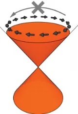
Solving Hψ = Eψ with H from Eq. (1.21), we obtain the dispersion relations E = ±α|~k|. In two spatial dimensions, this looks like a cone, the so-called Dirac cone.2 _{The Dirac cone and an} interpretation of the spin-momentum locking are illustrated in Fig. 1.15. The absolute value in

2_{The name comes from Paul Dirac.} _{He proposed the relativistic version of the Schr¨}_{odinger equation, which}

(26)

1.3. TOPOLOGICAL INSULATORS 19

E=±α|~k|is crucial here. The top cone has energyE=α|~k|, while the bottom cone has dispersion

E =−α|~k|. We note that this is fundamentally different from a dispersion without the absolute value, which describes to intersecting lines. Hence, at a fixed energy (e.g. the Fermi energy), we only have particles with one type of spin. 3

Figure 1.15: Schematic illustration of a Dirac cone. The black arrows denote the spin-momentum locking. Backscattering is not allowed. This is illustrated with the big grey arrow. From [29].

As already mentioned, the band inversion is a result of strong spin-orbit coupling. How are these two concepts related? The conduction and valence bands of a material can split for many different reasons. From a mathematical point of view, all these contributions are off-diagonal terms in the Hamiltonian. The largest contributions come from chemical bonds and crystal-field splitting (not relevant here). Finally, the much smaller contribution of the spin-orbit coupling pushes the levels closest to the Fermi level towards each other, reversing the two bands. This is illustrated schematically in Fig. 1.16. Hence, a topological insulator is the result of several splitting effects, of which strong spin-orbit coupling (strong enough to make them cross) is the most important one.

a

b

Splitting from other effects Splitting from SOC

[image:26.595.269.349.169.285.2]

E_F Band_inversion

Figure 1.16: Schematic representation of effects leading to the band inversion of the conductance band (a) and the valence band (b) in a topological insulator.

3_{Although this is usually referred to as “chirality” instead of spin. The chirality can be}_±_{1, depending on whether}

(27)

1.3.3 Weak antilocalisation

There are three types of electronic transport in solids, which can be classified by three characteristic lengths: `, `φ andL. The mean free path ` is the average distance an electron can travel before

being scattered by impurities. The phase coherence length `φ is the average distance the electron

travels before losing its phase coherence. Finally, the sample sizeLis the distance the electron has to travel. [33]

a If`L, electrons can pass through the sample without scattering, which we call it ballistic transport. The opposite case, when ` L, is known as diffusive transport. Usually we assume

`φ < `, such that phase does not play a role. However, if `φ `, electrons can maintain a phase

even after many scattering events. This is calledquantum diffusivetransport. [33]

Figure 1.17: Three types of electronic transport. From [33].

In the quantum diffusive regime, an electron can scatter around and come back to a location where it was before. Weak (anti)localisation is a correction as a result of electrons interfering with themselves after scattering off impurities in the material and returning to the initial position (i.e. after completing a closed loop). This interference can be both constructive or destructive. The former is called weak localisation and the latter is referred to as weak antilocalisation. In the case of topological insulators, we have weak antilocalisation which results from the strong spin-orbit coupling that we discussed in the previous section.

a Electrons travelling clockwise and counter-clockwise have opposite momentum, and because of spin-momentum locking, opposite spin as well. Hence, back-scattering (scattering to the direction where the electron came from) is suppressed, which leads to weak antilocalisation. [33]

1.4 Majorana particles

A Majorana particle is a particle that is its own antiparticle. This was hypothesized by Ettore Majorana in 1937. He suggested that some neutral (i.e. zero charge) spin-1₂ particles might be described by a real wave function. Since the wave functions of a particle and its antiparticle are related by complex conjugation, the two wave functions are identical. We note that the fact that they are neutral (i.e. zero charge) is crucial, since particles and antiparticles have opposite conserved charges (see Section 1.1.2). Put in second quantization operators, for a Majorana particle we have

ˆ

ck= ˆc†k. (1.23)

Expressed in words, removing a Majorana particle in statekis equal to creating a Majorana particle in state k. Recall that the antiparticle of an electron is a hole. We can think of a Majorana as an equal superposition of an electron and a hole. Since an electron has energyEand an hole is located

−E, we have

ˆ

(28)

1.4. MAJORANA PARTICLES 21

Hence, a Majorana particle is always located at zero energy. Since Majorana particles are part electron and part hole, a natural starting point to look for Majorana particles is in systems where both electron and hole quasi particle excitations occur; for example, in superconductors.

In an s-wave superconductor (that is, the standard superconductor that we have discussed so far), Cooper pairs consist of electrons with opposite spin. The annihilation operator of such an electron pair is

b=uc†_↑+vc↓, (1.25)

wherec†_↑ is the creation operator for a spin up particle andc↓is the annihilation operator for a spin down particle. The coefficients uandv can be interpreted as the weights in the electron and hole channel, respectively (see Section 1.2.3). Obviously,b6=b†. We slightly change the expression to

γ=uc†_σ+u∗cσ, σ∈ {↑,↓}. (1.26)

The quasi particle described by γ has equal electron and hole components, which have the same spin direction. We find thatγ=γ† and therefore,γ describes a Majorana particle.

1.4.1 Non-Abelian statistics

It turns out that Majorana particles always form pairs of the form

f = γ1+iγ2

2 , f

† ₌γ1−iγ2

2 . (1.27)

These pairs are constructed by means of a Kitaev chain [34] (which we will not discuss here), which results in two properties: they are degenerate and highly non-local. [35, 36] The first property, the degeneracy, implies that they always come in pairs (f andf†). This makes sense, since a Majorana particle is half electron and half hole, but “half an electron” does not exist. Having two of them solves this problem. The second property of being highly non-local implies that the pair of Majorana particles is spatially separated. Therefore, they are protected from local changes that only affect one of them, which implies that they are protected from decoherence. This causes the Majorana particles to be insensitive to environmental noise and suitable for quantum computing, as already touched upon in the Introduction.

We now consider exchanging the two particles in a pair. Quantum mechanically, we need to include all possible ways to do. The probability amplitude is given by the sum over all possible paths from one space-time point to another,

A= X

paths

exp

i Z t2

t1

L[~r1(t), ~r2(t)]dt

, (1.28)

where the integral represents a particular path. Most of these paths destructively interfere with each other. What remains is a contribution that can be written as a phase factor to the wave function, just like we already saw in Section 1.1.3:

(29)

Suppose we have N degenerate Majorana pairs. We can describe this state by the column vector

ψ= [ψ1 ψ2 . . . ψN]T. If we exchange two particles, the vector undergoes a linear transformation

(a rotation of the form of Eq. (1.6)) and arrives in another state in the same degenerate space, i.e.

ψ → U ψ, where U is an N ×N unitary matrix. If we interchange two other particles, we have the rotation ψ → V ψ, with V another unitary matrix. Since U and V do not commute (which usually is the case with matrix multiplication), the order of interchanging the particles determines the final state that we arrive in. [35] Say we have three particles, 1-2-3, and we want to get the state 2-3-1. If we first interchange 1-2 and then 2-3, this gives a different final state then if we were to interchange 1-3 and then 1-2 (see Fig. 1). This property is callednon-Abelian statistics and is crucial for applications in quantum computers, as already explained in the Introduction.

a Note that, in order to have non-Abelian statistics, we need to have at least 2 degenerate states (4 Majorana particles). Otherwise, the space is one-dimensional and therefore all linear transformations commute.

1.4.2 Two- and three-dimensional space

We can consider the probability amplitude from Eq. (1.28) in two or three dimensions and these will give quite different results. We consider three possible phases of the wave function in the cases of no exchange (A), single exchange (B) and two exchanges (C).

a We start with the three dimensional case as shown in Fig. 1.18a. Path A is closed and does not involve any exchange. Therefore, it can be shrunk to a point, which implies that the wave function cannot pick up a phase. Path B, with one exchange, has two different endpoints and cannot be shrunk to a point. This means that path B can result in a phase, which we callη. Path C contains two exchanges that form a loop. We can compare this with a string tied around a sphere, which we can also shrink into a point by tightening the string. Hence, two exchanges is equivalent to no exchange it all. This implies thatη2= 1, such thatη=±1. In three dimensions, we can only get bosons (η= 1) or fermions (η=−1), but no anyons.

A

B

C

(a) Three dimensional space.

A

B

C

(b) Two dimensional space.

Figure 1.18: Three types of paths. A: no exchange. B: single exchange. C: two exchanges.

(30)

1.4. MAJORANA PARTICLES 23

cannot be shrunk into a point. Therefore, we have a phaseη after one exchange, a phaseη2 after two exchanges, a phase η3 after three exchanges, and so on. Hence, the phase has to be η =eiφ, which explains why we can only get the anyon wave function in two dimensions.

a The mathematical crux lies in the study of the topology of these space, as already introduced in Section 1.3.1. The sphere in three dimensions has genus g = 0 (it is similar in shape to an “oliebol”), or, in mathematical terms, we can say that it is simply connected. Two dimensional space is not simply connected. This makes it possible to define paths that wind around the origin, resulting in the anyon behaviour. A full discussion on these spaces using homotopies (i.e. continuous deformations from pizzas to “oliebollen”) from three dimensions toZ2and from two dimensions to

Zis given in [35].

a The reason why we went through the hassle of relating Majorana behaviour to the topology of two and three dimensional space, is that it will turn out to be an important issue in the experiments that we will discuss in Chapter 4.

1.4.3 Superconductor / topological insulator junctions

We have now established the construction and importance of Majorana particles. The question that arises is, what kind of system supports their existence? From Eq. (1.26) it follows that we are looking for a superconductor where pairing between electrons with the same spin happens. This type of pairing is known as triplet pairing.4 _{Moreover, the structures of} _f _and_f† _{are (}_∼_γ

1±iγ2) are crucial here as well. The most obvious candidate to fit these two criteria is a chiral p-wave superconductor. In the superconductors we have considered so far, the ∆ parameter was a constant (see Section 1.2.3). In a chiralp-wave case, it is momentum dependent and has the structure

∆(~p) = ∆(px±ipy) = ∆e±iφ, (1.29)

where px and py are the momentum components in the xand y direction, respectively, and φ=

tan(py/px). This structure implies that the pair potential ∆ is rotating as a function of momentum.

The direction of the rotation can be either ±, which is called thechirality.

The most well known chiral p-wave superconductor is Sr2RuO4. However, it is very difficult to realise this material experimentally. Besides that, the actual pair potential remains a point of discussion and it is still not proven that Sr2RuO4 has indeed the pairing symmetry described by Eq. (1.29). [37]

a There are, however, other ways to induce triplet pairing in materials. A well known way to do so is using nanowires, which we will discuss in Section 4.1.1. Another possibility, which is the topic of interest here, is bringing a standards-wave superconductor (with a constant ∆ and Cooper pairs with opposite spin) in combination with a topological insulator.

When we first introduced the Majorana particle at the beginning of this section, we considered it as a particle that is half electron/half hole and that is located at zero energy. As discussed in Sec-tion 1.2.5, two superconductors with another material in between them can host an Andreev bound state (see Fig. 1.12a). If this bound state is located at zero energy, does that turn the Andreev bound state into a Majorana bound state? Almost.

a In the conventional case, the material in between the two superconductors is a normal metal, which has the parabolic dispersion relation that was shown in Fig. 1.8a. If the interfaces are abso-lutely perfect, an electron (without hole component) reflects as a hole (without electron component) and there is no interaction between the two bands. Therefore, there are states at zero energy, so in principle, this should work. In reality, however, the interfaces are not perfect. The two bands

4_{The name “triplet pairing” comes from the fact that there are three ways to pair electrons that are symmetric}

(31)

interact and a gap in the dispersion opens, comparable to the dispersion shown in Fig. 1.8b. The zero energy level lies inside this gap and therefore, it is impossible to have a Majorana bound state in this system. [29, 38]

a If we replace the normal metal in the middle by a topological insulator, this problem is solved. Recall that a topological insulator has spin-momentum locking (see Section 1.3.2) and therefore, backscattering is not possible. Hence, a particle inside the topological cannot go back; it can only go into the superconductor. Therefore, the transmission is equal to 1. We will see in Section 4.4.2 that this is a crucial property to host a Majorana particle.

a It can be shown mathematically that the spin-momentum locking of Eq. (1.21) with induced superconductivity results in the same energy spectrum as thepx+ipy superconductor. This idea

(32)

2

a

Modelling multiple Andreev

reflections

There are several ways to detect a Majorana particle. The most common ones are the use of nanowires and the 4π periodic current-phase relation. These two methods will be explained in Chapter 4, when we look at the experimental aspects of detecting a Majorana particle. In this chapter, we focus on yet another method, which considers multiple Andreev reflections (MAR).

a The concept of MAR was explained in Section 1.2.5. MAR occur in junctions with two super-conductors with a different material in between them. A superconductor/normal metal/superconductor (S/N/S) junction is called aconventional Josephson junction. If we replace the normal metal with a topological insulator, we have a superconductor/topological insulator/superconductor (S/TI/S) junction, which is referred to as atopological Josephson junction.

In Section 2.1, we will first discuss the rather simple resistively shunted junction model that has been used to model S/N/S junction. This model does not take MAR into account. The current through a one dimentional S/N/S junction as a result of MAR was first modelled by Averin-Bardas in 1995. Their model is discussed in Section 2.2. As a next step, we are interested in a junction with a topological insulator (TI) in the middle. When a TI is brought into contact with a superconductor, its surface becomes superconducting as well via the proximity effect. This combination of spin-momentum locking and superconductivity allows symmetry protected surface states to host Majorana particles; which has been a hot topic for the past decades. The one dimensional S/TI/S junction and its relation to Majorana particles were considered by Badiane, Houzet and Meyer in 2011. A brief review of their work is given in Section 2.3.

a The S/TI/S model showed a phenomena that is fundamentally different from the S/N/S junction. This is very interesting, however, it is not directly applicable to experiments. The reason is that experimental junctions cannot be considered one dimensional. The current can also flow through the junction under an angle, which makes the system two dimensional. The experimentally obtained result then corresponds to the current averaged over all possible angles. We expanded the existing one dimensional model to two dimensions to make an actual experimental prediction. By going to two dimensions, we are able to take the length of the TI, as well as the chemical potentials of both materials into account. Our expanded model is shown in Section 2.4.

(33)

26 CHAPTER 2. MODELLING MULTIPLE ANDREEV REFLECTIONS

is similar to the bound state in chiralp-wave superconductors.

2.1 The resistively shunted junction model

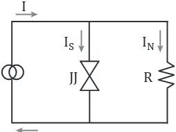
A frequently used tool to model S/N/S junctions is the resistively shunted junction (RSJ) model. In the RSJ model, a resistor (R) is put parallel to the S/N/S junction (J J), such that the current can be modelled as the sum of the supercurrentIS (the current in the absence of an applied voltage)

and the normal state currentIN (Ohmic behaviour). This is shown in Fig 2.1.

JJ R

IN

IS

[image:33.595.225.352.248.343.2]

I

Figure 2.1: Resistively shunted junction model.

The supercurrent has amplitudeIc (the critical current) and oscillates as a function of the phase

difference between the two superconductorsφ. In this simple model, the voltageV is given by the magnetic flux quantum (_~/2e) times the phaseφ. Summing the two contributions, we obtain

IRSJ=IS+IN =Icsinφ+ ~

φ

2eR. (2.1)

Because of its simplicity, this model is popular among experimentalists. However, it can only explain the experimental observations to some extent. The RSJ model does not take many physical aspects of the S/N/S junction into account. Especially the quantum properties are left out. For example, whereas the RSJ model gives a smoothI/V curve, experiments show an oscillating sub-harmonic gap structure (i.e. oscillations foreV <∆, where V is the applied voltage and ∆ is the superconducting gap).

a The main phenomenon that is responsible for the current in S/N/S junctions is the effect of multiple Andreev reflections (MAR), which will be the main topic of this chapter.

2.2 The S/N/S junction in 1D

Averin and Bardas [40] modelled the current through a S/N/S junction. They start by defining two additional regions I and II inside the superconductors, close to the interface (Fig 2.2). These regions represent the parts of the contact regions that are separated by the scattering region, where the motion of the quasi particles is possibly diffusive. The current through the junction is determined by the interplay of two effects: Andreev reflection at the interfaces with the superconductors, and scattering in the middle region. A short review of the work done by Averin and Bardas is discussed in this section.

We assume an incoming electron-like quasi particle from the left superconductor, which we model as J δn0. There is only one source at n= 0, which is why we use the Kronecker δ-function. The amplitude is given by J =p1−a2

(34)

[image:34.595.236.381.108.186.2]

2.2. THE S/N/S JUNCTION IN 1D 27

Figure 2.2: Schematic diagram of S/N/S junction. Image from [40].

there are four possible processes:

1. Reflection as an electron-like particle (normal reflection) Bn

2. Reflection as a hole-like particle (Andreev reflection) An

3. Transmission as an electron-like particle Cn

4. Transmission as a hole-like particle Dn

The letters behind these processes are the probabilities assigned to the occurrence of each pro-cess. After one of these processes has taken place, there will be a new particle approaching an interface and the same four processes can happen again. This is why we introduced the subscript

n. From Fig 1.12b, it becomes clear that in the case of Andreev reflection, the particle goes to a different energy level. This is taken into account by the Andreev coefficientan, which is defined as

an =a(ε+neV), wherea is given by Eq. (1.20). The full process that takes place in the S/N/S

junction is illustrated in Fig 2.3.

eV

E

S

N

N’

N

a0A0 a2A1

a4A2 B2

B1

B0 J

a2B0

C2

C1

C0 a1D0

a3D1 a5D2

Δ

-Δ ε

-ε ε + 2eV

ε + 4eV

-ε - 4eV

-ε - 2eV

ε + eV

ε + 3eV

ε + 5eV

-ε + eV

-ε - eV

-ε - 3eV

[image:34.595.138.480.431.688.2]

(35)

28 CHAPTER 2. MODELLING MULTIPLE ANDREEV REFLECTIONS

2.2.1 Wave functions

We are interested in the wave functions for holes and electrons in the regions I and II. We first consider the electrons in region I.

a2nAn J Bn

In this region, we have the source termJ, which is a right-going particle with momentumk. Since we assume a propagating particle, we multiply the source term byeikx. The reflected electron-like particleBngoes in the opposite direction,−k, hence, it is multiplied bye−ikx. To take all reflected

electron-like particles into account, we sum over n. After an even number of Andreev reflections, we get another right-going electron-like particle with amplitudea2nAn and momentumk.

What we discussed until now are all position dependent contributions to the wave function. However, the differential equation that we are dealing with also has a time derivative. Since the position dependent part and the time dependent part can be separated, we write the solution asψ(x, t) =

ψ(x)ψ(t). For the most standard form of the Schr¨odinger equation, the time dependent part is

e−iEt/~_{, where}_E _{is the energy and}_t_{denotes the time. In this case, every Andreev reflection shifts}

the energy level. The energy of an electron is increased by eV each time it passes through the channel from left to right. The energy of holes increases in the opposite direction; from right to left. Taking this together, we obtain the energy difference 2eV. Hence, the electron and hole wave functions are sums of components with different energies shifted 2eV. Taking all of these aspects into account, the electron wave function in region I can be written as

ψeI(x, t) =

X

n

(a2nAn+J δn0)eikx+Bne−ikx

e−i(ε+2neV)t/~_. _(2.2)

We can do the same for hole-like quasi particles in region I.

An

a2nBn

We have the Andreev reflected hole-like particlesAn that are propagating in the−k direction. If

a particle that was originally reflected as an electron (Bn) is then Andreev reflected at the next

interface, we obtain the right-going hole-like particlea2nBn. Similar to the previous case, the wave

function is given by the sum over all Andreev levelsn, multiplied by the same time dependent part. The wave functions becomes

ψ_hI(x, t) =X

n

Aneikx+a2nBne−ikx

e−i(ε+2neV)t/~_. _(2.3)

We move on to the electrons in region II.

Cn a2n+1Dn

If the source particle J is normally transmitted, it ends up in region II as a right-going electron-like particle with amplitude Cn. An Andreev reflected hole at the right interface ends up as an

electron-like particle in region II as well. This particle is denoted by a2n+1Dn. Because of the

energy difference eV in the middle (as seen in Fig 2.2), we now have to take the odd Andreev coefficientsa2n+1. This is also taken into account in the time dependent part. The electron wave function in region II is given by

ψ_eII(x, t) =X

n

Cneikx+a2n+1Dne−ikx

Interfaces of topological insulators and superconductors

䄀甀最甀猀琀

㄀ Ⰰ

㈀ ㄀㠀

䴀愀猀琀攀爀ᤠ

猀

吀栀攀猀椀

猀

䄀瀀瀀氀

椀

攀搀

倀栀礀猀椀

挀猀

☀

䄀瀀瀀氀

椀

攀搀

䴀愀琀栀攀洀愀琀椀

挀猀

䤀渀琀

攀爀昀愀

挀攀猀

漀昀

琀漀瀀

漀氀漀

最椀挀

愀氀 椀

渀猀甀

氀愀琀漀

爀猀 愀

渀搀

猀甀瀀

攀爀挀

漀渀搀

甀挀琀

漀爀猀

䰀椀渀

搀攀

䄀⸀䈀

⸀ 伀

氀搀攀

伀氀琀

栀漀昀

䜀爀愀搀甀愀琀椀

漀渀 挀漀洀洀椀

琀琀攀攀

䄀瀀瀀氀

椀

攀搀 倀栀礀猀椀

挀猀

倀爀漀昀

⸀

搀爀⸀

䄀⸀

䈀爀椀

渀欀洀愀渀

䐀爀⸀

䜀⸀

䠀⸀

䰀⸀

䄀⸀

䈀爀漀挀欀猀

䐀爀⸀

䌀⸀

䰀椀

䈀⸀

搀攀

刀漀渀搀攀Ⰰ

䴀⸀

匀挀⸀

䄀瀀瀀氀

椀

攀搀 䴀愀琀栀攀洀愀琀椀

挀猀

䄀瀀瀀氀

椀

攀搀 䴀愀琀栀攀洀愀琀椀

挀猀

Contents

Introduction

㄀　Ⰰ

㈀　㄀㠀

愀氀椀

爀猀愀

漀渀挀漀洀洀椀

攀搀倀栀礀猀椀

攀搀䴀愀琀栀攀洀愀琀椀

攀搀䴀愀琀栀攀洀愀琀椀