ISSN Online: 1947-3826 ISSN Print: 1949-2421
DOI: 10.4236/cn.2018.103005 Jul. 18, 2018 51 Communications and Network
Coarse Graining Method Based on Noded
Similarity in Complex Network
Yingying Wang, Zhen Jia
*, Lang Zeng
College of Science, Guilin University of Technology, Guilin, China
Abstract
Coarse graining of complex networks is an important method to study large-scale complex networks, and is also in the focus of network science to-day. This paper tries to develop a new coarse-graining method for complex networks, which is based on the node similarity index. From the information structure of the network node similarity, the coarse-grained network is ex-tracted by defining the local similarity and the global similarity index of nodes. A large number of simulation experiments show that the proposed method can effectively reduce the size of the network, while maintaining some statistical properties of the original network to some extent. Moreover, the proposed method has low computational complexity and allows people to freely choose the size of the reduced networks.
Keywords
Complex Network, Coarse Graining, Node Similarity, Statistical Properties
1. Introduction
Many complex systems in reality can be abstracted into complex networks [1] for research. Complex network has been one of the most active tools for the study of complex systems. It has important applications in many fields such as biology, economics and finance, as well as society, electricity, transportation and so on.
Since the similar topological properties of real-world complex networks, it is a hot topic to study the commonness of networks and the universal methods to deal with them [2]-[9]. However, many networks are known to exhibit rich. It is not enough to study the dynamic properties of small-scale networks, which may only reflect some local information of large-scale networks, while direct research on large-scale networks is computationally prohibitive. For example, the World-Wide-Web produces new web links every day. If the pages on the How to cite this paper: Wang, Y.Y., Jia, Z.
and Zeng, L. (2018) Coarse Graining Me-thod Based on Noded Similarity in Com-plex Network. Communications and Net-work, 10, 51-64.
https://doi.org/10.4236/cn.2018.103005
Received: May 24, 2018 Accepted: July 15, 2018 Published: July 18, 2018
Copyright © 2018 by authors and Scientific Research Publishing Inc. This work is licensed under the Creative Commons Attribution International License (CC BY 4.0).
DOI: 10.4236/cn.2018.103005 52 Communications and Network World-Wide-Web are thought of as the nodes and the hyperlinks between them as edges, then the World-Wide-Web is a huge complex network and continues growing. It is difficult to deal with this kind of large-scale networks, coarse graining of complex networks is the latest way to overcome such difficulty in the world. Given a complex network with N nodes and E edges, which is considera-bly large and hard to be delt with, the coarse-graining technique aims at map-ping the large network into a mesoscale network, while preserving some topo-logical or dynamic properties of the original network. This strategy is based on the idea of clustering nodes with similar or same nature together.
In the past decade, some well-known coarse-graining methods have been proposed [10]-[21]. Historically, these methods can be classified into two cate-gories: one is based on the eigenvalue spectrum of the network. Its main goal is to reduce the network size while keeping some dynamic properties of the network. For example, D. Gfeller et al. proposed a spectral coarse-graining algorithm (SCG) [11] [12], Zhou and Jia proposed an improved spectral coarse-graining algorithm (ISCG), Zeng and Lü proposed a path-based coarse graining [13] [14]. All these coarse-graining methods are developed to maintain the synchronization ability. Another coarse-graining method is based on topological statistics of the network, for instance, the k-core decomposition [10], the box-counting techniques [15] [16], the geographical coarse-graining method introduced by B. J. Kim, et al. in 2004. And referring to literature [18], the network reduction is related to seg-menting the central nodes by impleseg-menting the k-means clustering techniques, etc. These methods can well maintain some of the original networks. In 2018, our research team proposed a coarse-graining method based on the generalized degree (GDCG) [19]. Specifically, the GDCG approach provides an adjustable ge-neralized degree by parameter p for preserving a variety of significant properties of the initial networks during the coarse-graining processes.
DOI: 10.4236/cn.2018.103005 53 Communications and Network small-world networks, SF networks reveal that the proposed algorithms can ef-fectively preserve some topological properties of the original networks.
2. Definition of Node Similarity
Consider a complex network G=
(
V E,)
consisted of N nodes, where V is theset of nodes and E is the set of edges. The adjacency matrix A a=
( )
ij describes the topology of the network. In general,a
ij=
1
indicates the presence of an edge, whilea
ij=
0
stands for the absence of edges. For an undirectedun-weighted network, whose adjacency matrix A must be symmetric matrix, i.e.
ij ji
a a
=
and the sum of the i’th row (or the i’th column) elements of the matrix A is exactly the degree ki of the node i. Here we use the Jaccard similarity in-dex to calculate the similarity between node pairs. The similarity between any node i and node j in the network is defined as:( )
( )
( )
( )
, ij i j s i jΓ ∩ Γ
=
Γ ∪ Γ (1) Let Γ
( )
i denote the set of neighbor nodes of node i, Γ( )
i is the cardinali-ty of the set Γ( )
i . Mathematically, Γ( )
i =ki. Γ( )
i ∩ Γ( )
j is the common neighbor node set of node i and j,Γ( )
i ∪ Γ( )
j is the union of the neighbor nodes of node i and j. By Equation (1),s
ij=
s
ji, it shows that the similarity with the node i itself is 1. And if the node i and the node j have no common neighbor nodes, then their similarity is zero, i.e.,s
ij=
0
,so0
≤ ≤
s
ij1
. Becauses
ij de-scribe the degree of local structure similarity between the node i and j. We treatij
s
as the local similarity index.The similarity between the node i and other nodes in the network can be ex-pressed by a Ndimension vector si =
(
s si1, , ,i2 siN)
T. The larger the value1
N ij j= s
∑
is, the more nodes in the network are locally similar to the node i. There-fore, we extend the Equation (1), the global similarity index for node i in the network is defined as follows:1 . N i ij j gs s =
=
∑
(2)
The larger gsi is, the more likely the node i will be the cluster center of some similar nodes.
3. Noded Similarity Coarse-Graining Scheme
It is noted that coarse-graining methods have to solve two main problems: one is the emergence of nodes, that is, to determine which nodes should be merged; And the second is how to update the edges in the process of coarse graining. In the following content, the noded similarity coarse-graining scheme is introduced from these two sides.
3.1. Nodes Condensation Based on Similarity Index
DOI: 10.4236/cn.2018.103005 54 Communications and Network one with N (N N < ) nodes. First, we need to select N cluster center, per-form the clustering algorithm to get the corresponding N cluster, then merge nodes in the same cluster.
In order to select N suitable nodes as the cluster centers, it is necessary to ensure that the extracted cluster centers have as much high global similarity as possible (with as many nodes as possible in the network). It is also required that the local similarity between the two clustering centers should not be too high (otherwise, they may belong to the same cluster, only one of them could be the clustering center).
The detailed steps for selecting N clustering are shown as follows.
Step 1: Get the local similarity and the global similarity of each node in the network. The sequence gs gsv1, v2, , gsvN of the generalized degree of N nodes has been sorted in decrease order.
Step 2: Set VS be the set of cluster centers. Firstly, put the node v1 which
cor-responding to the maximum global similarity gsv1 into VS, denoting VS =
{ }
v1 .Secondly, pick the node v2 corresponding to the second largest global similarity
2
v
gs , if
1 2
v v N s
N β
< × (N and N are the size of the coarse-grained networks and original networks respectively, β is an adjustable parameter). It indicates that the node v2 and v1 are not in the same cluster, so v2 could be the
second cluster center. Push v2 into VS, denoting VS =
{
v v1, 2}
. Otherwise, if1 2
v v N s
N β
≥ × , which means that the local similarity between the node v2 and
1
v is too high and these two nodes may belong to the same cluster. Then v2 cannot be put into VS as a new cluster center. Continue to select the cluster centers in the order of gs gsv1, v2, , gsvN, the new cluster center node vi has to satisfy: v vi j
N s
N β
< × ,
v V
j∈
S. In this way, stop selecting the new cluster centersuntil the number of VS reaches N, denoting VS =
{
v v1, , ,2 vN}
.Step 3: Take
v v
1, , ,
2
v
N as the cluster centers respectively, theircorres-ponding clustering sets are described as
M M
1,
2, ,
M
N. And then cluster theremaining N N− nodes in the network (the collection of the remaining nodes is represented as:
V V V
S= −
S). In order to find the clustering setM
j that the node vi of theV
S belong to, our objective is to find:2
min i j
j S i S v v
v V v V∈
∑
∈ s −s (3) where, svi (svj) is corresponding to the local similarity of the node vi (v
j) with other nodes in the network. svi−svj 2 is the L2 norm between nodesi
DOI: 10.4236/cn.2018.103005 55 Communications and Network
3.2. Updating Edges of the Reduced Networks
N clustering sets have been obtained from the section 3.1, merge nodes in each cluster and get N coarse-grained nodes. To keep the connectivity of the re-duced network, the following step is to update edges, the detailed content is as following:
Definition of weight. The set of nodes in ith cluster is defined as Mi (Mi is also the ith node in coarse-grained networks). We re-encode the weight, specifi-cally:
, , , 1,2, , , ,
i j
i j
M M ij
i M j M
W a i j N i j
∈ ∈
=
∑
= ≠ (4)where,
a
ij is the element in the adjacency matrix A a=( )
ij of the original network. And WM Mi j is the weight of the edge between node Mi andM
j.Definition of edge. The edge eM Mi j between nodes Mi and
M
j is defined by:(
)
0 max ,
1 otherwise i j
i j
M M i j
M M
N
W M M
e N < =
(5) , i j
M M separately represent the number of the nodes in ith, jth cluster. As presented above, the framework can preserve the edges between the clusters (each cluster corresponds to a coarse-grained node) that are closely related to each other in original networks. Moreover, it can prevent the network from re-ducing into a fully connected network. And removing the weight of the edges, only displaying the topology structure of the coarse-grained networks, is condu-cive to keep some statistical properties of the original networks. In particular, if the network becomes disconnected after deleting the edge eM Mi j, then recon-nect the edge eM Mi j in order to ensure the connectivity of the network. Now we can create an undirected unweighted network after two steps as described above.
3.3. A Toy Example
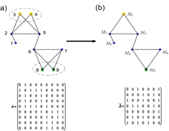
To better illustrate the algorithm we proposed, this section will apply the noded similarity coarse-graining scheme on the small toy network, as shown in Figure 1.
A 9-node toy example is shown in Figure 1(a). Here, we use the noded simi-larity coarse-graining method to reduce the network into 7 nodes, and β =0.7
to meet the required coarse-grained network size. First of all, calculate and sort the global similarity of nodes in decrease order as
3, 4, 8, 9, 5, 6, 1, 7, 2
gs gs gs gs gs gs gs gs gs . It can be found that: gs3=gs4=3.1 and
8 9 2.65
gs =gs = . Intuitively, the two yellow circular nodes like the two green diamond nodes have totally equal topological roles. According to step 2 of sec-tion 3.1, put the largest global similarity node 3 into the set VS, namely, node 3 is the first cluster center corresponding the clustering set M1. Then take the
node 4 to compare with the cluster center node 3. From the Equation (1),
( )
3( ) { }
4 2,5Γ = Γ = , 34 1 7 0.7 9
DOI: 10.4236/cn.2018.103005 56 Communications and Network
Figure 1. A toy example based on the node similarity coarse-graining method. (a) A 9-node simple network with adjacency matrix A; (b) The reduced network with adjacency matrix A.
cluster center into to the set VS . And so on, the set of cluster center
{
3,8,5,6,1,7,2}
S
V = with the collection of the remaining nodes VS =
{ }
4,9 canbe obtained, while each element in VS corresponds to the clustering sets:
1, 2, 3, 4, 5, 6, 7
M M M M M M M . It is not difficult to calculate
4 3 9 8
2 2
0
v v v v
s −s = s −s =
∑
∑
according to Equation (3). The distance betweenthe node 4 and the cluster center node 3 is the smallest one, so the node 4 should be merged with the cluster center node 3 together. They belong to the same clustering set M1; akin to the node 4, the node 9 and the cluster center node 8
belong to the same clustering set M2. At this point, seven coarse-grained nodes
have been obtained. There are only 0, 1 or 2 three kinds of weight between the coarse grained nodes. So take the node M M5, 7and node M M1, 3 as an
exam-ple to update edges. By Equation (4), WM M5 7 =1, WM M1 3 =2, following the
definition in Equation (3), WM M5 7 =1>79max
(
M5 ,M7)
=97,(
)
1 3 1 3
7max , 14
9 9
2
M M M M
W = > = , so eM M5 7 =1, eM M1 3 =1. For the nodes
that are not connected in the original network, their edge weight are still set to 0 in the coarse-grained network. Then we can create the coarse grained network with adjacency matrix A, as shown in Figure 1(b).
4. Numerical Demonstrations
[image:6.595.194.538.62.327.2]DOI: 10.4236/cn.2018.103005 57 Communications and Network the average path length, average degree and clustering coefficient. Recently, the average path length, average degree and clustering coefficient are the three most concerned topological properties in the research of complex networks. They de-scribe more explicit information about the various aspects in the networks. Spe-cifically, we will give a clearer definition in the following sections. And for sim-plicity, we main consider three typical networks (the ER random networks, the WS small-world networks and the SF scale-free networks). To better illustrate the effect of the proposed method on these topological properties. We investi-gate our method with different values of β. On the other hand, under the op-timal β, we further investigate the effect with the structural parameters of dif-ferent networks. For simplicity, we consider the ER random networks with con-necting probability p=0.01, 0.02, 0.03, 0.04, 0.05. The WS small-world net-work algorithm is proposed by Newman and Eatts in 1998, which is obtained by randomly rewiring each edge of the original networks on the basis of the near-est-neighbor coupled networks. We adjust the rewiring probability with
0.1, 0.2, 0.3
p= and coordinator number K=4, 6, 8. In terms of SF networks, the degree distribution follows the power-law distribution. When the power-law exponent
γ
increases from small to large, the power-law networks change from the highly heterogeneous networks to the highly homogeneous networks. Sinceγ
typically lies between 2 and 3 for many real-world systems. We main consider the cases with γ =2.05, 2.25, 2.5, 2.75, 3.Additionally, for each type of the artificial complex networks, we fix the size of these networks as N=1000, and for each type of the typical complex net-works, we consider N =1000, 900, 800, 700, 600, 500, 400, 300, 200,100. The results of all the illustrated experiments are the average of ten independent si-mulation runs.
4.1. Average Path Length
The average path length L between two nodes is defined by:
(
)
1 21 i j N ij
L d
N N ≤ < ≤ =
−
∑
(6) where N is the size of the network,
d
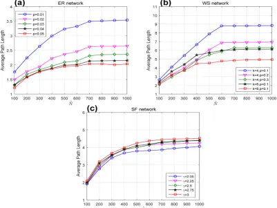
ij is the shortest path length from i to j.Figure 2 & Figure 3 show the evolution of the average path length of the above mentioned networks with noded similarity coarse-graining method. From Figure 2(a), one can see that for the ER networks the average path lengths are almost the same with the adjustable parameter β varying from 0.1 to 0.6. It means that the value of β does not have a great impact on the ER networks. Therefore, we randomly pick β=0.6 to get the results shown in Figure 3(a).
Under each p, the average path length can be well preserved, especially for
700
N ≥ . For the WS networks, when 600≤N ≤800, the larger β is, the better effect of maintaining the average path length will be. And the curve with
1.1
DOI: 10.4236/cn.2018.103005 58 Communications and Network
Figure 2. Evolutions of the average path length under different β. (a) ER network; (b) WS networks; (c) SF networks.
[image:8.595.98.500.401.702.2]DOI: 10.4236/cn.2018.103005 59 Communications and Network different rewiring probability p and coordinator number K. For the SF networks under optimal β =0.5, the average path length is better maintained with
2.75,N 700
γ
≥ > as shown in Figure 3(c).4.2. Average Degree
Average degree k is a critical index to weigh the relatively connectedness of the whole network. Given the adjacent matrix A of a network, the corresponding
k is given by:
1 1
N N
i ij ji
i i
k A A
= =
=
∑
=∑
(7)1 1 N
i i
k k
N =
=
∑
(8)
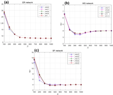
The evolutions of average degree k versus the parameter β with the node similarity coarse-graining processes for the three types of networks are shown in Figure 4. Similar to the phenomenon exists in Figure 2, ER random networks are not sensitive to different values of β. For the WS networks, the curves under β=0.9,1,1.1 are obviously better than β=0.7, 0.8 in
[image:9.595.140.531.371.699.2]preserv-ing the clusterpreserv-ing coefficient of the original networks with 200≤N ≤600. And the effect of keeping the clustering coefficient is better with a relatively smaller
DOI: 10.4236/cn.2018.103005 60 Communications and Network β in the SF networks.
As displayed in Figure 5, the average degree can be preserved in three kinds of coarse-grained networks with the optimal β. In ER networks, the curve of average degree is approximately linear with p=0.01,N>500. With the
in-crease of p, the volatility of the curve increases, but it also roughly keeps the av-erage degree. From Figure 5(b), the average degree for all WS networks can be well preserved regardless of the structural parameters. In SF networks, the node similarity algorithm can better keep the average degree of the original networks with the increase of
γ
. Moreover, the average degree of the coarse grained net-works is within 1 degree relative to the average degree of original netnet-works even the size of the original networks is reduced to half. As you can see, the SF networks are superior to the above two networks in maintaining the average degree.4.3. Clustering Coefficient
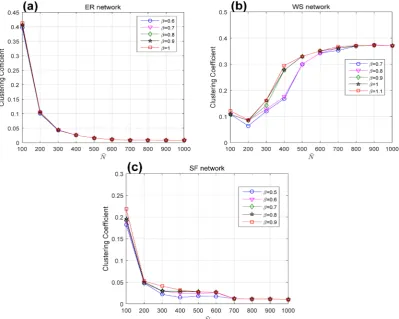
[image:10.595.148.540.324.691.2]The clustering coefficient measures the edge connection probability between the neighbor nodes in a network. The clustering coefficient Ci of node i with the
DOI: 10.4236/cn.2018.103005 61 Communications and Network average degree ki is defined as:
(
2 i 1)
ii i
E C
k k
=
−
(9)
where Ei gives actual number of edges between ki neighbor nodes of node i. The overall level of clustering in a network is measured as the average of the clustering coefficients of all nodes:
1 1 N
i i
C C
N =
=
∑
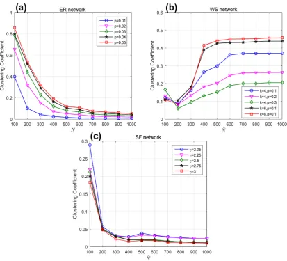
(10) [image:11.595.122.522.380.699.2]The result shows that the optimal parameter β corresponding to the best performance on preserving different statistical properties is the same. From the result shown in Figure 7(a), when the connecting probability p increase, the ef-fect of maintaining the clustering coefficient in ER networks becomes more prominent. Whenp>0.03,N =100, the clustering coefficient of coarse-grained networks are in the range of 0.8 which agree with the plan of updating edges. The WS networks are typically with high clustering coefficient. The curves tend to decrease sharply with the increase of K and the decrease of the rewiring proba-bility p. When N is less than the threshold value 200, all curves turn to rise. But in general, the clustering coefficient of the original networks can be effectively maintained of certain structural parameters. In Figure 7(c), different curves
DOI: 10.4236/cn.2018.103005 62 Communications and Network
Figure 7. Evolutions of the clustering coefficient under different structural parameters. (a) ER network; (b) WS networks; (c) SF networks.
coincide with each other especially N >500. Which indicate that the clustering coefficient property can be well preserved in the SF networks.
5. Conclusions and Discussions
DOI: 10.4236/cn.2018.103005 63 Communications and Network
Acknowledgements
This project is supported by National Natural Science Foundation of China (61563013, 61663006) and the Natural Science Foundation of Guangxi (No. 2018GXNSFAA138095).
References
[1] Watts, D.J. and Strogatz, S.H. (1998) Collective Dynamics of “Small-World” Net-works. Nature, 393, 440-442. https://doi.org/10.1038/30918
[2] Barabási, A.L. and Albert, R. (1999) Emergence of Scaling in Random Networks. Science, 286, 509-512. https://doi.org/10.1126/science.286.5439.509
[3] Barabási, A.L., Albert, R. and Jeong, H. (1999) Mean-Field Theory for Scale-Free Random Networks. Physica A: Statistical Mechanics and Its Applications, 272, 173-187. https://doi.org/10.1016/S0378-4371(99)00291-5
[4] Pan, Z.F. and Wang, X.F. (2006) A Weighted Scale-Free Network Model with Large-Scale Tunable Clustering. Acta Physica Sinica-Chinese Edition, 55, 4058-4064. [5] Li, H., Li, Z.Y. and Lu, J.A. (2006) Weighted Scale-Free Network Model with
Evolving Local-World. Complex Systems and Complexity Science, 3, 36-43. [6] Dörfler, F., Chertkov, M. and Bullo, F. (2013) Synchronization in Complex
Oscilla-tor Networks and Smart Grids. Proceedings of the National Academy of Sciences, 110, 2005-2010. https://doi.org/10.1073/pnas.1212134110
[7] Qin, J., Gao, H. and Zheng, W.X. (2015) Exponential Synchronization of Complex Networks of Linear Systems and Nonlinear Oscillators: A Unified Analysis. IEEE Transactions on Neural Networks and Learning Systems, 26, 510-521.
https://doi.org/10.1109/TNNLS.2014.2316245
[8] Tang, L., Lu, J. and Chen, G. (2012) Synchronizability of Small-World Networks Generated from Ring Networks with Equal-Distance Edge Additions. Chaos: An Interdisciplinary Journal of Nonlinear Science, 22, 023121.
https://doi.org/10.1063/1.4711008
[9] Zhou, T., Zhao, M. and Wang, B.H. (2006) Better Synchronizability Predicted by Crossed Double Cycle. Physical Review E, 73, 037101.
https://doi.org/10.1103/PhysRevE.73.037101
[10] Alvarez-Hamelin, I., Dall’Asta, L., Barrat, A. and Vespignani, A. (2005) K-Core Decomposition: A Tool for the Analysis of Large Scale Internet Graphs. cs. NI/0511007.
[11] Gfeller, D. and De Los Rios, P. (2007) Spectral Coarse Graining of Complex Net-works. Physical Review Letters, 99, 038701.
https://doi.org/10.1103/PhysRevLett.99.038701
[12] Gfeller, D. and De Los Rios, P. (2008) Spectral Coarse Graining and Synchroniza-tion in Oscillator Networks. Physical Review Letters, 100, 174104.
https://doi.org/10.1103/PhysRevLett.100.174104
[13] Zhou, J., Jia, Z. and Li, K.-Z. (2017) Improved Algorithm of Spectral Coarse Grain-ing Method of Complex Network. Acta Physica Sinica, 66, 060502.
[14] An, Z. and Lv, L.Y. (2011) Coarse Graining for Synchronization in Directed Net-works. Physical Review E, 83, 056123. https://doi.org/10.1103/PhysRevE.83.056123
[15] Song, C., Havlin, S. and Makse, H.A. (2005) Self-Similarity of Complex Networks. Nature, 433, 392-395. https://doi.org/10.1038/nature03248
DOI: 10.4236/cn.2018.103005 64 Communications and Network
Complex Networks. Physical Review Letters, 96, 018701.
https://doi.org/10.1103/PhysRevLett.96.018701
[17] Kim, B.J. (2004) Geographical Coarse Graining of Complex Networks. Physical Review Letters, 93, 168701. https://doi.org/10.1103/PhysRevLett.93.168701
[18] Xu, S. and Wang, P. (2016) Coarse Graining of Complex Networks: A K-Means Clustering Approach. 2006 Chinese Control and Decision Conference (CCDC), Yinchuan, 28-30 May 2016. https://doi.org/10.1109/CCDC.2016.7531703
[19] Long, Y.S., Jia, Z. and Wang, Y.Y. (2018) Coarse Graining Method Based on Generalized Degree in Complex Network. Physica A Statistical Mechanics & Its Applications. https://doi.org/10.1016/j.physa.2018.03.080
[20] Chen, H., Hou, Z., Xin, H. and Yan, Y. (2010) Statistically Consistent Coarse-Grained Simulations for Critical Phenomena in Complex Networks. Physical Review E, 82, 011107. https://doi.org/10.1103/PhysRevE.82.011107