Measuring management practices
Manthos D. Delis, Mike G. Tsionas
PII: S0925-5273(18)30095-1
DOI: 10.1016/j.ijpe.2018.02.006
Reference: PROECO 6956
To appear in: International Journal of Production Economics
Received Date: 22 August 2017 Revised Date: 13 January 2018 Accepted Date: 8 February 2018
Please cite this article as: Delis, M.D., Tsionas, M.G., Measuring management practices, International Journal of Production Economics (2018), doi: 10.1016/j.ijpe.2018.02.006.
M
AN
US
CR
IP
T
AC
CE
PT
ED
Measuring Management Practices
February 10, 2018
Manthos D. Delis
Montpellier Business School, 2300 Avenue des Moulins, 34080 Montpellier, France, [email protected]
Mike G. Tsionas
M
AN
US
CR
IP
T
AC
CE
PT
ED
Measuring Management Practices
Abstract
Good management practices are remarkably difficult to robustly measure, especially when unique
data on firms and their managers are not available. We propose a new model estimated with
Bayesian techniques that requires only the usual accounting data on inputs and outputs and thus
can be applied to any firm. We show that our management practices estimates are more than
90% correlated with existing state-of-the-art measures from a very specialized data set by Bloom
and Van Reenen (2007). We also obtain very high correlations when conducting an extensive
Monte Carlo analysis. Finally, we show that frontier-based methods previously used to estimate
management practices do not provide good approximations.
M
AN
US
CR
IP
T
AC
CE
PT
ED
1
Introduction
The robust quantification of good management practices (also termed managerial quality, skill, ability,
or simply management) is an indispensable tool of empirical research in management, economics,
fi-nance, and other social sciences. Measuring management practices poses well-known difficulty, mainly
due to the scarcity of relevant disaggregated data and the mere nature of the concept, and the relevant
literature goes back to Mundlak (1961), Lucas (1978), and Rosen (1981), who note that differences in
firm productivity must be related to the so-called firm fixed effect of managerial quality. In more recent
endeavors, Bloom and Van Reenen (2007; 2010) use survey data to assess good management practices
of firms, while Demerjian et al. (2012; 2013) and Bonsal IV et al. (2016) use data envelopment
anal-ysis (DEA)-based methods. Other studies use either measures of inventory buffers of manufacturing
firms (e.g., Lieberman et al., 2005) or corporate governance characteristics related to experience (e.g.,
Custódio et al., 2017).
Relative to this literature, the contribution of our study is twofold. First, we propose a new method
to thoroughly measuregeneral management practices and show, through several validation methods,
that we have come the closest yet to their approximation. Second, our method can be applied to any
firm without posing restrictions on data availability, besides the usual output and inputs of production
that can be derived from simple financial statements. This is highly important because our approach
can be applied to all firms for which conventional accounting data are available.
Our method relies on the estimation of a simple cost efficiency model, where management is an
input of production. This approach is consistent with a broad definition of management practices,
which includes human and intellectual capital, conceptual and technical skills, and entrepreneurial
and human-resource abilities that lead to better management of the traditional inputs and superior
productivity (Katz, 1974; Bloom et al., 2017). Thus, this broad set of management practices
encom-passes virtually all other inputs, besides labor and capital, used by firms to achieve their objectives.
The novel element of our research is that management is an unobserved (latent) variable (input of
production) to be estimated from the data. The drawback of our approach is the somewhat more
involved statistical procedure, as we must use Bayesian econometrics due to the presence of several
latent variables in our model.
Our model yields a system of five equations to be simultaneously estimated. The first two equations
are a translog cost function and one of the share equations that is related to unobserved management
practices. The share equation is used to allow identification of management from the cost-share
system. The third and fourth equations estimate the determinants of the unobserved managerial price
(compensation) and management practices, respectively. These latent variables are approximated only
M
AN
US
CR
IP
T
AC
CE
PT
ED
technical efficiency, which is allowed to depend on latent management. This is important from a
theoretical viewpoint because management quality must be a significant part of technical efficiency.
We systematically explore the internal validity of our model using (i) a unique data set previously
employed to robustly measure management practices and (ii) 1,000 simulated data sets generated from
a production function. First, in a series of milestone papers for the measurement of management
practices, BVR (2007; 2010) and Bloom et al. (2012) use a rigorous interview-based evaluation tool
that examines the basic managerial practices covering all relevant processes of firms. This yielded
the World Management Survey (WMS), which is an international research initiative to measure the
differences in management practices across organizations and countries. In summary, the WMS’s
methodology is to obtain and conduct interviews with senior managers across a number of dimensions
in firm performance, ensure the collection of accurate responses through several procedures, and
eval-uate management practices across operations management, performance monitoring, target setting,
leadership management, and talent management.1 To the best of our knowledge, the WMS produces
the most detailed and scientifically-based measure of management practices, albeit for a limited number
of medium-sized firms.
In addition to the measurement of management practices, BVR report data on the usual inputs
(capital and labor) and output (sales) of firms. This data set allows us to conduct an experiment to
validate our estimates. We first estimate our model using data only on firms’ output and inputs from
BVR (2007) and obtain estimates for management practices. Subsequently, using a simple bivariate
regression, we compare our estimates with the BVR scores and find that our estimates explain about
92% of the BVR scores.
In turn, we examine whether this high correlation holds in other samples by conducting a Monte
Carlo study. To make the environment relatively unfavorable to our model and more favorable to
existing frontier-based methods for the measurement of management practices, we generate panels from
a production function with simulated information on inputs and their prices, output, and management
practices. We use different sizes of the cross-sectional dimension (firms) and a constant time dimension,
as well as different assumptions regarding availability of data for the input prices. We show that as the
cross-sectional dimension of the sample increases (eventually reaching a maximum of 2,500 firms over
10 years), the rank correlations between our model’s estimates and simulated management scores are
between 0.83 and 0.91, depending on whether information on the two input prices is available (larger
values observed when data on both input prices are available). Thus, our two validation procedures
show that we have come very close to a robust measure of management practices.
As a final exercise, we check how the measurement of management practices from Data Envelopment
M
AN
US
CR
IP
T
AC
CE
PT
ED
Analysis (DEA) fares when applied to the data set of BVR (2007). The application of a
DEA-based method to measure management is currently the most common approach in the literature (e.g.,
Demerjian et al., 2012). The premise of that literature is that management is part of the efficiency
component, which is estimated using DEA. Management can then be derived as a residual from the
regression of DEA scores on variables that managers cannot affect (e.g., firm size, market share, firm
age, etc.). This technique has gained momentum despite the fact that it involves regressing the DEA
scores on covariates, a practice that biases results in unknown magnitude and direction (as highlighted
in the seminal paper of Simar and Wilson, 2007).
We first apply the usual DEA approach (Demerjian et al., 2012; 2013; Bonsal IV et al., 2016) to
the same output and inputs from BVR (2007) and use as management practices either these scores
or the residuals from the regression of the DEA scores on firm size, firm age, etc., as management
practices. Subsequently, we compare the DEA-based management scores with those from BVR. We
find that DEA-based measures are statistically significant determinants of the BVR scores but never
explain more than 5% of these scores.
Besides the work by BVR (2007; 2010) and Bloom et al. (2012; 2017), our paper relates to several
strands of literature in a multidisciplinary context. The common aim of these strands is to identify
sources of productivity differences of firms and sources of managerial quality (e.g., Sáenz-Royo and
Salas-Fumás, 2014) and, to this end, it is important to have a robust measure of management practices
that can be applied to any firm. Unless there is access to unique and specialized data, the unobserved
(stochastic) nature of management unavoidably leads to some sort of econometric/mathematical
anal-ysis.
The literature (predominantly the management literature) stresses quite graphically the
impor-tance of validation of any new measure of management practices. Only indicatively, Schriesheim et
al. (1993) identify deficiencies in the measurement of management practices and suggest that any new
method requires some sort of validation based on good benchmark data. Schilke and Goerzen (2010)
conceptualize and operationalize alliance management capability, and contribute to the performance
effects of alliance structures and alliance experience based on survey data from 204 firms. Richard et
al. (2009) focus on measuring organizational performance and conclude with a call for research that
examines triangulation using multiple measures, longitudinal data, and alternative methodological
formulations as methods of appropriately aligning research contexts with the measurement of
organi-zational performance.” Even more recently, Hermalin and Weisbach (2017) discuss the importance of
managerial ability and its assessment in firms’ corporate governance.
Our paper proceeds as follows. In Section 2 we present our model and estimation approach. In
M
AN
US
CR
IP
T
AC
CE
PT
ED
directions for future research.
2
Unobserved management
2.1
Model
We consider a production model of the firm in which management practices, x∗
J, is an unobserved
(latent) input of production. The recent work of Bloom et al. (2017) motivates the modeling of
management as a factor of production. We aim to model x∗
J using a cost-share system, plus two
equations that allow the identification of management practices and their price, respectively, from
their latent dynamics and other observed variables. We also add a fourth equation to the model to
allow for a firm inefficiency component and its dependence on management and other variables (e.g.,
Sáenz-Royo and Salas-Fumás, 2014).
An important question is whether management is the only unobserved input of production. If it is
not, thenx∗J will capture other inputs unrelated to managementper se. There are two main reasons
backing our assumption, the first theoretical and the second driven by our empirical results. First,
management science broadly defines management practices to include human and intellectual capital,
conceptual and technical skills, and entrepreneurial and human-resource abilities leading to better
management of the traditional inputs and superior firm productivity (Katz, 1974; many others since
then). Indeed, the coordination of the rest of the inputs involves precisely these broadly defined skills
to gather, allocate, and distribute economic resources or consumer products to individuals and other
businesses in the economy. This definition is also fully aligned with standard microeconomic theory,
which assumes that there is a third factor of production besides labor and capital (including land).
Specifically, all modern economic textbooks list human capital, entrepreneurship, or a similar notion
as a factor of production (e.g., Samuelson and Nordhaus, 2009). Management practices, as defined
here, encompass all of these notions and, thus, it should be only this “best management practices”
component missing from the list of firms’ inputs in the estimation of production relations.
Second, our empirical results essentially back our assumption that management is the main (if not
the only) unobserved input of production. Our key validation approach compares our estimates from
the model below to the state of the art measure of management practices developed by BVR (2007).
The approach of this study is to obtain unique survey data on a specific sample of firms for which
best management practices are well-defined and measured. This approach has nothing to do with
the estimation of a production relation, so that identifying a close relation between our estimates of
management practices and those of BVR constitutes a strong indication that what we indeed measure
M
AN
US
CR
IP
T
AC
CE
PT
ED
We begin with a cost function of the form:
C=C(w1, ..., wJ−1, w∗J, y) = min x∈RJ
+
: w′x,s.t. F(x, y) = 1, (1)
wherew= [w1, ..., wJ−1, wJ∗] ′
is the vector of input prices,y is the vector of outputs,xis the vector of
inputs, andF is a transformation function. Here, we consider the case of one output (the log of sales),
and two observed inputs, namely labor (the log of employees) and capital (the log of capital stock) as,
for example, in Bloom and Van Reenen (2007) and Chen et al. (2015). The choice of a cost function is
in line with the premise that managers seek to achieve a given level of output by minimizing costs. Also,
w∗
J is the (usually) unobserved (latent) management price (average managerial compensation across
firms) of management practices,x∗
J, andC=w1x1+...+wJ−1xJ−1+wJ∗x∗J ≡T Cx+wJ∗x∗J, where
T Cxdenotes the input cost excluding management cost (cost of labor and capital). For simplicity, let
w= [w1, ..., wJ−1]′be the vector of input prices besides management price (i.e., the prices of labor and
capital). We treat all input prices as parameters of inputs to be estimated and thus constant across
firms.2
We have the following share equations and, as in similar modeling frameworks (e.g., McElroy, 1987;
Hijzen et al., 2005), we can drop the second one:
wjxj
T Cx+w∗
Jx∗J =
∂logC(w,w∗
J,y)
∂logwj , ∀j= 1..., J−1,
w∗
Jx∗J
T Cx+w∗
Jx∗J =
∂logC(w,w∗
J,y)
∂logwJ .
(2)
For simplicity, and without loss of generality, let us consider the case of one output and two inputs
(J = 2), the second of which is management practices. Using a translog specification, which is the
preferred in many empirical exercises due to its flexibility and linearity in parameters (Greene, 2008),
we have:
log C
w1 =βo+β1(logw
∗
2−logw1) +12β2(logw∗2−logw1)2+
+β3logy(logw∗2−logw1) +β4logy+12β5(logy)2.
(3)
The share equation corresponding to management is:
S2∗=β1+β2(logw∗2−logw1) +β3logy. (4)
Thus, we haveC=w1x1+w∗2x∗2 andS2∗= w∗
2x∗2
w1x1+w∗2x∗2 = 1−S1.
In (4) the dependent variable corresponding to managerial share will always be observed asS∗ J =
1−PJ−1
j=1Sj. Further,w∗2 can be identified through the nonlinearity in (3) and the joint appearance
2Despite the fact that some databases (e.g., BoardEx) report managerial salaries or the price of capital, we are
M
AN
US
CR
IP
T
AC
CE
PT
ED
ofw∗
2 in (3) and (4). The technical problem, however, is thatx∗2 appears also inC and thus we need
assumptions on predetermined variables that identifyx∗
2 andw∗2 to be stated in additional equations
below.
For all firms and time periodsJ−1, the econometric (stochastic) form of the cost function and the
first share equation is as follows:
Cit=C wit, wJ,it∗ , yit;β+v1,it+uit, wj,itxj,it
T Cx
it+w∗J,itx∗J,it
=∂logC(wit,w∗J,it,yit;β)
∂logwj,it +vj,it, ∀j= 1..., J−1,
(5)
whereβis the parameter vector to be estimated,vit= [v1,it, ..., vJ+1,it]′is the vector of error terms, and
uit≥0 represents technical inefficiency. The addition of the error terms in our model follows standard
practice in the estimation of stochastic production relations (e.g., Coelli et al., 2005; Kumbhakar and
Lovell, 2000). This essentially implies decomposing the stochastic term to the inefficiency component
and the remainder disturbance, which captures random shocks outside the control of firms. For the
error terms in (5), we assume vit ∼ NJ(O,Σ), ∀i = 1, ..., n, t= 1, ..., T.As is also standard in the
same literature,vitis independent fromuit, and we impose concavity in input prices and monotonicity
(e.g., Kumbhakar and Lovell, 2000; Coelli et al., 2005).
Technical inefficiency comes, as usual, from the result that cost inefficiency is related to
input-oriented inefficiency (Kumbhakar, 1997). To impose linear homogeneity with respect to prices, we
express all prices relative to the first one. Besides the variables reflecting output and inputs, we use
country and industry dummies in the cost equation, as we find that these improve the precision of our
management practices estimates relative to our validation benchmarks.
For the measurement of the latent variables, we assume that
logw∗Jt=µ1(1−ρ1) +ρ1logw∗J,t−1+x′tα1+εt1, ∀t= 1, ..., T, (6)
logx∗J,it=µ2i(1−ρ2) +ρ2logx∗J,i,t−1+x′itα2+εit,2, ∀i= 1, ..., n, t= 1, ..., T. (7)
In equations (6) and (7) µ1, µ2 and ρ1, ρ2 are, respectively, location and persistence parameters for
the variables involved. Ifρj = 1 then the intercept µj disappears. Separate identification is possible
because (i)µ2andρ2appear in the denominator of the left hand side of (7) and (ii) there is a separate
first order condition (equation 7), which involves onlyw∗
Jt in the right hand side of (6). In equation
(6) we keep, for simplicity, managerial compensation equal across all firms (as we do for the rest of the
input prices) and only allow it to vary with time.3 This does not affect our estimates but considerably
eases estimation. In contrast, management practices in equation (7) varies with both firm and time,
M
AN
US
CR
IP
T
AC
CE
PT
ED
as this is the main focus of our analysis.
Importantly, equations (6) and (7) allow the identification of our two main variables from observed
characteristics and a dynamic latent variable (i.e., unobserved persistence of management practices
and their price). As is usual the case with panel data, the degree of persistence is expected to be
‘large’; thus we do not consider this a strong assumption. In essence, we place more structure on
management practices and their price to come up with well-identified posterior measures.4 This is also
well-justified theoretically because learning-by-doing processes, personnel and director experience,
la-bor immobility, restrictive regulations and wage stickiness, etc., create important sources of persistence
in the management practices of firms.5
Symmetrically withw∗
Jt, we havext=n−1Pni=1xit. In the vectorsxandx, of equations (6) and
(7), we include firm size (measured by the log of fixed assets),6 its squared term to capture potential
non-linear effects due to diseconomies of scale, the principal component of prices on labor and capital
and its square, and the interaction of firm size with the principal component. We allow management
and managerial compensation to depend on these variables and especially the principal component of
the price of labor and capital because part of an effective management is to determine the right input
prices. Of course, the alternative would be to have both prices in each specification. Unfortunately,
adding more latent variables in the model yields convergence problems. With the principal component,
the model runs and yields the results reported in the paper. Of course, the “success” of our analysis
is outcome-driven: we use this approach because results are closer to Bloom and Van Reenen and the
ones produced in our Monte Carlo exercise.
For the error terms in (6) and (7), we assumeεt1∼ N 0, σ2ε1
, εit,2∼ N 0, σε22
,∀i= 1, ..., n, t=
1, ..., T. The multivariate normality assumptions, along with the relevant ones in equation (5), are
standard practice in the econometric literature (e.g., Coelli et al., 2005; Kumbhakar and Lovell, 2000).
A final key element of our model is that we allow the technical inefficiency component to depend
on management practices, as follows:
uit∼ N+ a0+a1x∗Jt+a2ui,t−1+a′zit, σ2u
, ∀i= 1, ..., n, t= 1, ..., T. (8)
4Surely, we have distributional and parametric assumptions, which, however, we believe are reasonable based on prior
grounds. Also, their validity should be considered in light of the evidence we provide. If the validation procedures showed that our estimates of management practices were questionable, we would have had to think again about the entire specification. For example, non-persistent managerial ability estimates would make us wonder why this is so and our attention would turn to the specification of the model. As the results on persistence are highly significant and our management scores are a very good fit to the scores of BVR and the scores from the Monte Carlo simulations, we proceed with the simplest assumptions possible that are also in line with existing literature.
5Bloom and Van Reenen (2010) show that management practices persist and attribute this persistence to the reasons
we highlight. For implications of persistence of managerial quality within a framework of innovation, see Custódio et al. (2017). Wage stickiness and its causes is analyzed in a big economics literature (e.g., Goette et al., 2007; references therein).
6For firm size, we would optimally require the total firms’ assets, but as these are not available, we use fixed assets.
M
AN
US
CR
IP
T
AC
CE
PT
ED
Equation (8) is a fundamental model in efficiency and productivity analysis, since at least the work of
Kumbhakar et al. (1991) and Battese and Coelli (1995), who consider the role of external determinants
of inefficiency. From a theoretical viewpoint, Bloom et al. (2017) discuss the role of efficiency in the
production function, noting the role of dynamics in this component. The dependency of the
ineffi-ciency component on management practices is intuitive from a theoretical viewpoint as management
is considered to be part of the overall firm efficiency (e.g., Demerjian et al., 2012; 2013; Koester et
al., 2016). The difference here is that management quality is a (latent) variable to be estimated and
thus the relation between management and inefficiency is testable in our context (i.e., whethera1 is
significant). In the vector,z, which denotes the variables affecting firm inefficiency, we include firm
size and its square, a time trend and its square to capture trends in efficiency, as well as interactions
of size with trend and ui,t−1. Note that we also allow for dynamic inefficiency, which is important
given the high persistence of inefficiency within firms for reasons similar to persistence in management
practices and compensation (also see, Bloom et al., 2017).
In a nutshell, our complete model to be estimated includes equations (5) to (8). As in the inefficiency
literature, we also provide definitions of managerial and cost-inefficiency elasticities (even though these
are not strictly part of the model). We define managerial elasticity as:
ϑit=
∂logC wit, w∗J,it, yit
∂logw∗ J,it
, ∀i= 1, ..., n, t= 1, ..., T, (9)
which represents the responsiveness of total costs to a change in management price. We also define
the elasticity of cost inefficiency with respect to management practices (i.e., the responsiveness of cost
inefficiency to a change in management practices) as:
ηit=
∂logE(uit|Dit)
∂logx∗ J,it
, ∀i= 1, ..., n, t= 1, ..., T, (10)
whereDit denotes all data andE(uit|Dit) is the usual measure of technical inefficiency (Jondrow et
al., 1982). This elasticity can be computed using numerical derivatives. The rest of the variables are
as in the equations (5) to (8).
2.2
Estimation using Bayesian techniques
We use a Bayesian technique based on Sequential Monte Carlo/Particle-Filtering (SMC/PF), the
theoretical details of which are described in the appendix.7 The reason we use this approach is that we
must include dynamic latent variables in our model. We introduce the dynamics because we believe
that persistence is an important part of variables like management practices and their price. When
M
AN
US
CR
IP
T
AC
CE
PT
ED
dynamic latent variables are present, the likelihood is not available in closed form because of the
presence of multivariate integrals with respect to the latent variables. There are no reliable procedures
for approximating multivariate integrals and thus the likelihood cannot be accurately approximated.
SMC/PF techniques precisely deal with this problem and they offer unbiased and consistent (in the
number of simulations) estimates of the likelihood and posterior.
Our prior for the translog parameters and those in associated share equations is the “vague prior”,
β ∼ N 0, 104I
. We adopt the same prior for α1, α2, a0, a1, and a. For µ1 and µ2i, we assume
µ1 ∼ N(0, 1), µ2i ∼ N(µ, σµ2), ∀i = 1, ..., n, where µ ∼ N(0, 1). For ρ1 and ρ2, we assume a
uniform prior U(−1,1). For Σ, we assume p(Σ) ∝ |Σ|−(m+1)exp −1 2trAΣ
−1
, with m = 1 and
A = 10−4I. All scale parameters σ2 ε1, σ
2 ε2, σ
2
u, and ω2 follow proper but vague priors of the form
p(σ) ∝ σ−(n+1)exp− q 2σ2
, and we set n = 1, q = 10−4. For notational simplicity we let θ =
[β′,α′
1,α′2,a, µ1, µ]′,
First, we write (5) as follows:
F(wit, wJ,it∗ ;yit,β) =vit+uitι, (11) whereι= [1,0, ...,0]′,v
it∼ N(0,Σ). The posterior distribution is given by:
p(β,θ, µ, σε1, σε2, σu, σµ,Σ,{uit},{logw∗J,t−1},{logx∗J,i,t−1}|D)∝ |Σ|−(J+m+1)exp
−1
2tr (A+S)Σ −1 ·
σ−ε1(nT+1)exp n
−2σ12
ε1
P i=1
PT
t=1 logwJt∗ −µ1(1−ρ1)−ρ1logwJ,t∗ −1+x′tα1 2o
·
σ−ε2(nT+1)exp n
− 1 2σ2
ε1
P i=1
PT
t=1 logx∗J,it−µ2i(1−ρ2)−ρ2logx∗J,i,t−1−x′itα2 2o
·
σu−(nT+1)exp n
− 1 2σ2
u
P i=1
PT
t=1(uit−a0−a1x∗Jt−a2ui,t−1−a′zit)2 o
·
Qn i=1
QT t=1Φ
a0+a1x∗Jt+a2ui,t−1+a′zit
σu
−1
·
σµ−(n+1)exp n
−2σ12
µ
Pn
i=1 µ2i−µ 2o
·p β,θ, µ, σε1, σε2, σu,Σ,
(12)
whereS=P
i=1
PT
t=1Vit(wit, wJ,it;yit,β),
Vit(wit, wJ,it;yit,β)≡ F(wit, wJ,it∗ ;yit,β) = "
Cit−C wit, wJ,it∗ , yit;β−uit,
wj,itxj,it
T Cx
it+w∗J,itx∗J,it
−∂logC(wit,w∗J,it,yit;β) ∂logwj,it
J
j=2 #′
,
(13)
and the prior appears in the last line of (12).
To implement Markov Chain Monte Carlo we draw from the following conditional distributions of
scale parameters, which are in standard form:
q+P i=1
PT
t=1 logw∗Jt−µ1(1−ρ1)−ρ1logw∗J,t−1+x′tα1 2
σ2 ε1
M
AN
US
CR
IP
T
AC
CE
PT
ED
q+P i=1
PT
t=1 logx∗J,it−µ2i(1−ρ2)−ρ2logx∗J,i,t−1−x′itα2 2
σ2 ε2
∼χ2
nT+n, (15)
q+Pn
i=1 µ2i−µ 2
σ2 µ
∼χ2n+n. (16)
Forσ2
u we draw a candidate:
q+P i=1
PT
t=1(a0+a1x∗Jt+a2ui,t−1+a′zit)2
σ2 u
∼χ2nT+n, (17)
and we accept the candidate with probability: Qn i=1
QT t=1Φ
a
0+a1x∗Jt+a2ui,t−1+a′zit
σu
−1
as
given in the fifth line of (12). Moreover, we drawµusing:
µ∼ N n−1 n X
i=1
µ2i, n−1σµ2 !
. (18)
To facilitate SMC/PF, we integrateΣout of the posterioranalytically(see Zellner, 1971, p. 355).8
The only difference is that the first line of the posterior in (12) now becomes:{det (A+S)}−(nT+m+1)/2.
We use 120,000 iterations of the SMC/PF algorithm, discarding the first 20,000 to mitigate possible
start up effects (starting values are generated randomly from the prior). We use 106 particles per
iteration. To integrate out the latent variables{uit},{logw∗J,t−1},{logx∗J,i,t−1}and draw parameters
we use the following procedure:
• Step 1: Integrate out the latent variables using Part A2 in Appendix A.
• Step 2: Draw parametersβusing Part A1 in Appendix A.
The Appendix contains also introductory and supporting material for implementing these steps, in
some detail.
3
Validation
3.1
Comparison with the scores from the World Management Survey
Our first and most important validation approach is to compare our management estimates with those
of BVR, obtained from the WMS data. Here we refer mostly to BVR (2007), who use a sample covering
6,267 observations (panel data). In our estimations, we use 6,049 observations given data availability
8The result is as follows. If the posterior is p(β,Σ|D) ∝ |Σ|−(N+1)/2exp
−12trA(β)Σ−1 , then p(β|D) =
R
p(β,Σ|D)dΣ =|A(β)|−(N+1)/2, whereβis the parameter vector,Ddenotes the data, integration is with respect to
the different elements ofΣ,N =nT+m, andA(β) =A+P
i,tvit(β)vit(β)
′, wherevit(β)denotes residuals from
M
AN
US
CR
IP
T
AC
CE
PT
ED
on required variables.9 Importantly, BVR provide information on accounting data that are employed
as inputs and output in our model and for the variables included in the vectorsx, x, and z. Thus,
by using these variables, we can estimate the system of equations (5) to (8) and then compare our
management practices estimates with the BVR scores.10 This forms an ideal experiment to validate
our results.
Table 1 reports summary statistics for the output/inputs. The log of sales (output) has a mean
value equal to 11.83 and a standard deviation of 1.44. The log of capital (input 1) has a mean of 10.11
and a standard deviation of 1.68, while the respective values for the log of employees (input 2) are 6.73
and 1.33. All three variables are positively skewed and leptokurtic, reflecting a high clustering around
the mean values (and hence a relatively low standard deviation).
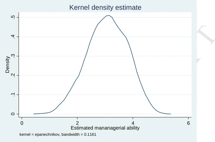
Reporting results for the all-too-many parameters from the translog system of equations is
im-practical; we thus only report summary statistics for our management practices estimates in Table 1
(against those of BVR) and provide a graphical representation (Kernel density) of our results in Figure
1.
[Insert Table 1 here]
[Insert Figure 1 here]
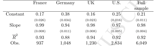
Our first step toward validation is to regress our estimated scores against those of BVR. From doing
this, we obtain the results in Table 2. We run regressions separately for firms in France, Germany,
UK, and U.S., as well as for all countries jointly (full sample). We note that we estimate our model of
equations (5) to (8) only once to take full account of information and underlying heterogeneity.
[Insert Table 2 here]
As shown in Table 2, the correlation of our estimates with the BVR scores is quite impressive
despite the fact that we have used none of the extra information available in the BVR data set (like
noise and general controls, college degree of manager, other attributes of the manager, etc.). The slope
in all regressions is close to unity and equal to 0.98 in the regression on the full sample, indicating
an almost one-to-one response of the BVR estimates to our estimates. Importantly, the R-squared of
the regressions is also higher than 0.9 in all samples but the German one, reaching a value of 0.92 in
the full sample. Further, in Figure 2, we provide a graphical comparison of our scores versus those of
BVR. The fit is remarkably good with very few outliers. In a nutshell, our estimates of management
practices almost perfectly predict those of BVR.
9This data set is freely available here:
http://worldmanagementsurvey.org/survey-data/download-data/download-survey-data.
M
AN
US
CR
IP
T
AC
CE
PT
ED
[Insert Figure 2 here]
Even though our validation so far is made via one database, we cannot really attribute the fit to
luck. Of course, our results are still an approximation to BVR (which are also subject to small error),
but this approximation is surprisingly accurate and the BVR data are perhaps the best approximation
of management practices in the literature. Thus, we must conclude that our method produces very good
estimates of management practices, while having the great advantage that can be applied to any data
set with accounting information only on inputs/outputs and firm size.
3.2
Monte Carlo simulation
In this section, we conduct further validation tests using repeated random sampling. The main reason
we conduct this validation is to examine the fit of our results in samples outsides that of BVR. To
make the environment relatively unfavorable to our model and more favorable to existing
frontier-based methods for the measurement of management practices, we do not consider a cost function, but
rather a production function of the formY =F(K, L, E) =KαLβEγexp(ν−u), whereK,L, andE
stand for capital, labor, and intermediate inputs, whose relative prices arewK,wL, andwE. We set
α= 0.20,β = 0.60, andγ = 0.15. Moreover,ν is the error term anduis technical inefficiency. We
assumeu= 1−M, whereM is management practices. The maximum value ofM is 1, so that when
M = 0 we haveu= 1 and whenM = 1 we haveu= 0. The elasticity of inefficiency with respect to
management is−M
u =
M M−1 ≤0.
We normalize the price of output to unity and we generate relative prices of capital, labor, and
intermediate inputs as uniform numbers in the interval (1, 10), (0.1, 1), and (0.1, 5), respectively. We
generate technical inefficiency asu∼N+(0, σu2), whereσu = 0.3 andv ∼ N+(0, σv2) whereσv = 0.3,
so that the signal-to-noise ratioλ= σu
σv = 1. Then, we generate values for M fromu= 1−M. The
unobserved management pricew∗
M is a positive function of managementw∗M = 10Mexp(εM), where
εM ∼ N(0, 0.12).
Evidently, in our Monte Carlo setup, management is part of the inefficiency component and not
directly an input of production as in our baseline model. The reason for this choice is to make
the Monte Carlo environment less favorable to our model and more favorable to the literature that
estimates management practices using standard frontier efficiency methods. In this way, we actually
give an initial advantage to the frontier approaches. Please note, however, that our Monte Carlo setup
is consistent with the modeling of management practices as an input. The reason is that M still
enters the Monte Carlo production function as a multiple of the standard inputs via the inefficiency
componentu.
M
AN
US
CR
IP
T
AC
CE
PT
ED
K= αY
wK, L=
βY wL, E=
γY
wE. (19)
For management practices the first order condition is:
KαLβEγexp(ν−u) =w∗
M. (20)
Substituting the first order conditions in the production function, we can generate output as:
Y = ( α wK α β wL β γ wE γ
exp (v−u)
)1−(α+β+γ)
. (21)
Then, we can generate input values from equation (12). For realism, we consider error terms so
inputs are generated in stochastic form as follows:
K= αY
wK
exp(εK), L=
βY wL
exp(εL), E=
γY wE
exp(εE), (22)
whereεK, εL, εE∼ N 0, σ2inp
, σ2
inp= 0.1 The unobserved management price can be generated from
equation (13) with the following minor modification:
KαLβEγexp(ν−u) =w∗Mexp εw∗
M
, (23)
whereεw∗
M ∼ N
0, σ2 w∗
M
,σ2 w∗
M = 0.1. We use 1,000 replications. In all cases the time periods are set
toT = 10, but the number of firmsnvaries as shown in the results reported in Tables 3 and 4.
Subsequently, we re-estimate our model of equations (5) to (8) using the simulated data. We
consider four different estimations (cases) based on whether input pricesw are observed or not. In the
first case, we assume that all input prices are observed, in the second thatwL is latent, in the third
that wL and wK are latent, and in the fourth that all wL, wK, and wE are latent. In Table 3, we
report summary statistics for the simulated and estimated management scores and for the different
sample sizes. Evidently, the values of means and standard deviations of the estimated management
practices are very close to the simulated ones, especially as the sample size increases and some of the
input prices are observed.
Importantly, in Table 4 we report rank correlations of simulated and estimated management
prac-tices (first row of each sample sizen and in bold), rank correlations of simulated and estimated
man-agerial elasticity (second row of each sample size) and rank correlations of simulated and estimated
managerial price (third row of each sample size). We also report results from four different assumptions
M
AN
US
CR
IP
T
AC
CE
PT
ED
wK, and missing all three prices).
[Insert Tables 3&4 here]
The results show that as the number of firms increases, we obtain higher values for the rank
correlations between the simulated and estimated management practices. Where all prices are observed
andn = 2,500, the correlation reaches 0.91; where all prices are missing, the respective correlation is
still as high as 0.83. These results hold despite the fact that our simulated samples are drawn from a
production function (results would be even more favorable if we drew samples from a cost function).
In a nutshell, and following validation via the sample of BVR, the Monte Carlo study also suggests a
very good fit of our model’s estimates to simulated management practices scores. This should hold in
most real samples, given that most sample sizes from databases such as Orbis and Compustat will be
higher thann = 2,500 x 10 years, especially with respect to the cross-sectional dimension.
3.3
DEA methods against robust existing measures
Most existing studies on the measurement of management practices use the implications of the large
frontier efficiency literature to draw implications. The premise of this literature is that good
man-agement is part of technical efficiency of firms, at least as far as the reach of managers goes to affect
managerial operations. Most of the management literature uses DEA techniques, a set of inputs and
outputs, and some transformation of the end technical efficiency DEA scores to estimate management
practices. Subsequently, these estimated management practices scores are used to examine relations
between management practices and other variables (e.g., Demerjian et al., 2013). Unfortunately, these
two-stage techniques are rarely validated using rigorous statistical methods and, as research has shown,
are prone to significant error. Importantly, Simar and Wilson (2007; 2011) demonstrate that when
DEA efficiency scores are simply regressed on covariates, inference is biased and inconsistent.11
Without aiming to condemn existing studies in their entirety, we carry out validation of a
DEA-based approach against the sample of BVR. DEA efficiency is usually defined as the ratio of outputs
over inputs. The particular DEA method we use is the same as in Demerjian et al. (2012). Specifically,
we solve the following optimization problem:
maxθ=y∗(υκx)−1, (24)
subject toθ≤1,κ= 2 inputs, andυ >0 is a parameter denoting the relative weight of the inputs in
11Many studies discuss this problem and propose solutions. For reviews, see Bădin and Daraio (2011) and Olesen and
M
AN
US
CR
IP
T
AC
CE
PT
ED
production. We use DEA on the same firms as in our previous exercise and the same output (sales)
and inputs (capital and labor). Given that firms do not usually operate at optimal scale (because
of regulations, imperfect competition, credit constraints, etc.), we resort to a variable-returns-to-scale
model. This implies that we add a convexity constraint to the DEA model (see e.g., Coelli et al., 2005,
pp. 172). Finally, to be consistent with our previous analysis in answering by how much can input
quantities be proportionally reduced without changing the output quantity, we use an input-oriented
DEA model. We run all DEA models using the standard software of Coelli (1996).
We first use three different DEA scores: (i) DEA applied once to the full sample, (ii) DEA applied
four times by country, and (iii) DEA applied numerous times according to the 2-digit industry SIC
code. In column (1) of Table 5 we use the first of these scores to predict the management practices
scores of BVR. The slope is highly statistically significant, but the fit of the regression is less than
1%. In column (2) we use the country-specific DEA scores, which increase the R-squared to 2.5%. In
column (3), we use the industry-specific DEA scores and this further improves the R-squared to 5.1%.
[Insert Table 5 here]
In column (4), we use a procedure similar to that of Demerjian et al. (2012). We first estimate
DEA by industry and then regress DEA on firm size, firm age, a dummy reflecting whether the firm is
public or not, and a dummy reflecting whether the CEO is the founder. These potential correlates of
firm efficiency are variables beyond the control of managers and might need to be cleaned out to receive
better estimates of management practices. In turn, we use the residuals as management practices. We
find that the slope is still highly significant, but the R-squared is again as low as 4%. Also, the fit of
this regression to the management practices estimates of BVR is relatively loose (Figure 3). Of course,
the management practices estimates are correlated with firm performance measures like Tobin’s q, etc.,
and in this respect the validation tests by Demerjian et al. (2012) are well done. What we suggest
here is that DEA-based scores can at best be viewed as correlates of management practices and not
as good estimates of management practices.
[Insert Figure 3 here]
Of course, there is a big list of DEA models that can be applied to measure management practices
and, undoubtedly, some of them will provide a better fit to the BVR scores. We especially expect that
stochastic DEA methods will provide better results, because these methods at least partially overcome
the problem raised by Simar and Wilson (2007). Our objective in this paper, however, is to compare
our method with existing methods. As our method yields good results, we leave the examination of
M
AN
US
CR
IP
T
AC
CE
PT
ED
4
Concluding remarks and directions for future research
Measuring management practices has been at the center of research in management and economics
for many years. In our research, we estimate a simple model of the firm, that is completely aligned
with microeconomic theory, where management practices is an unobserved (latent) variable (input
of production). The use of latent variables requires estimation via an admittedly involved Bayesian
method. The rents are, however, quite satisfactory: using data only on inputs (labor and capital),
output (sales), and firm size, we are able to predict by approximately 92% the "actual" managerial
quality scores of Bloom and Van Reenen (2007). The latter scores are a quite accurate reflection
of management practices, as they have been drawn from a very careful analysis of survey data. We
also validate our estimates using simulated data drawn from a production function and show that
the estimates of management practices still closely predict the actual management practices scores,
especially as the sample size increases. Finally, we show that DEA-based methods, currently the
predominant way of estimating management practices, provide a much poorer fit.
We view our findings as particularly important in two dimensions. First, to the best of our
knowl-edge, we have come the closest yet to the robust measurement of general management practices. By
general here we mean the full spectrum of firm managerial processes that affect firm productivity,
efficiency, and performance. Thus, we view our method as an advancement to the frontier-based
methods that decompose the firm inefficiency component to a management component and a
resid-ual. Given that the fit of our method is better according to an extensive set of validation techniques,
we suggest that our model allows better future research on multiple fields, especially in economics
and management, but also in finance, accounting, even in sociology, psychology, and other social and
applied sciences. Second, the model presented in this paper can be used for closely approximating
management practices in panels or cross sections of firms without the need of detailed data: simple
accounting ratios are sufficient. Thus, our method can be applied to all firms in the world, for which
simple accounting data are available.
Our model can be extended to allow for testing several theories in the fields of management (e.g.,
management practices and innovation as in Custódio et al., 2017; or agency problems as in Mutlu et
al., 2017), finance (e.g., management practices and risk as in Bonsall IV et al., 2016; value creation
in M&As as in Delis et al., 2017), economics (e.g., along the lines of the work of Bloom and Van
Reenen, as already discussed; the value of management in the short- and long-run processes of firms
as in Sáenz-Royo and Salas-Fumás, 2014), and accounting (e.g., management practices and earnings
quality as in Demerjian et al., 2013; tax avoidance as in Koester et al., 2016). Further, a similar model
including latent variables can be applied to other difficult-to-measure notions, such as corporate social
M
AN
US
CR
IP
T
AC
CE
PT
ED
considerable ground, we leave these for future research.
APPENDIX
In this appendix, we discuss the theoretical details of the Bayesian estimation methodology (particle
filtering) used in Section 2.2 to obtain management practices estimates. Note that this discussion
is intended to provide the econometric theory behind the precise particle filtering used and allow
the reader to be located with respect to that theory. The discussion here appeared previously in an
unpublished mimeo entitled “Estimating management and its applications” by Tsionas (2016), which
we replicate as Tsionas (2016) is not available online.
Particle filtering
The particle filter methodology can be applied to state space models of the general form:
yT ∼p(yt|xt), st∼p(st|st−1), (A.1)
wherestis a state variable. For general introductions, see Gordon et al. (1993), Doucet et al. (2001),
and Ristic et al. (2004).
Given the dataYt, the posterior distribution p(st|Yt) can be approximated by a set of (auxiliary)
particlesns(ti), i= 1, ..., .N o
with probability weightsnw(ti), i= 1, ..., N o
, where PN i=1w
(i)
t = 1. The
predictive density can be approximated by:
p(st+1|Yt) = Z
p(st+1|st)p(st|Yt)dst≃ N X
i=1
p(st+1|s(ti))w (i)
t , (A.2)
and the final approximation for the filtering density is:
p(st+1|Yt)∝p(yt+1|st+1)p(st+1|Yt)≃p(yt+1|st+1) N X
i=1
p(st+1|s(ti))w (i)
t . (A.3)
The basic mechanism of particle filtering rests on propagatingns(ti), w (i)
t , i= 1, . . . , N o
to the next
step, viz. ns(ti+1) , wt(+1i) , i= 1, . . . , No, but this often suffers from the weight degeneracy problem.12 As
is often the case that parameters θ ∈ Θ ∈ ℜk are available, we follow Liu and West (2001), where
12This is a problem of the weights produced by older versions of SMC/PF. Specifically, a few weights were close to
M
AN
US
CR
IP
T
AC
CE
PT
ED
parameter learning takes place via a mixture of multivariate normals:
p(θ|Yt)≃ N X
i=1
w(ti)N(θ|aθt(i)+ (1−a)¯θt, b2Vt). (A.4)
In (A.4), ¯θt = PNi=1w (i) t θ
(i)
t , and Vt = PNi=1w (i) t (θ
(i)
t −θ¯t)(θt(i)−θ¯t)′. The constants a and b are
related to shrinkage and are determined via a discount factor δ ∈ (0,1) as a = (1−b2)1/2 and
b2= 1−[(3δ−1)/2δ]2.On this, see also Casarin and Marin (2007).
Andrieu and Roberts (2009), Flury and Shephard (2011), and Pitt et al. (2012) provide the Particle
Metropolis-Hastings (PMCMC) technique. This technique uses an unbiased estimator of the likelihood
function ˆpN(Y|θ), as p(Y|θ) is often not available in closed form.
Part A1. Parameter propagation
Given the current state of the parameterθ(j) and the current estimate of the likelihood, say Lj =
ˆ
pN(Y|θ(j)), a candidateθcis drawn fromq(θc|θ(j)), yieldingLc= ˆpN(Y|θc) . Then, we setθ(j+1)=θc
with the Metropolis - Hastings probability
A= min
1, p(θ
c)Lc
p(θ(j)Lj
q(θ(j)|θc q(θc|θ(j))
. (A.5)
Otherwise, we repeat the current draws
θ(j+1), Lj+1 =
θ(j), Lj .
Hall et al. (2014) propose an auxiliary particle filter, which rests upon the idea that adaptive particle
filtering (Pitt et al., 2012) used within PMCMC requires far fewer particles to approximate p(Y|θ)
compared to the standard particle filtering algorithm. From Flury and Shephard (2011) we know that
auxiliary particle filtering can be implemented easily once we can evaluate the state transition density
p(st|st−1). When this is not possible, Hall et al. (2014) present a new approach, wherest=g(st−1, ut)
for a certain disturbance. In this case, we have:
p(yt|st−1) = Z
p(yt|st)p(st|st−1)dst, (A.6)
p(ut|st−1;yt) =p(yt|st−1, ut)p(ut|st−1)/p(yt|st−1). (A.7)
If one can evaluate p(yt|st−1) and simulate from p(ut|st−1;yt), the filter would be fully adaptable
(Flury and Shephard, 2011).
We can use a Gaussian approximation for the first-stage proposalg(yt|st−1) by matching the first
two moments ofp(yt|st−1). So the approximating density p(yt|st−1) = N(E(yt|st−1),V(yt|st−1)). In
M
AN
US
CR
IP
T
AC
CE
PT
ED
possibility that it is multimodal (as it turned out so in the course of using SMS/PF) and thus we assume
it hasM modes with ˆum
t , for m= 1, . . . , M. For each mode, we can use a Laplace approximation. If
we letl(ut) =log[p(yt|st−1, ut)p(ut)], from the Laplace approximation we obtain:
l(ut)≃l(ˆutm) +12(ut−uˆ m
t )′∇2l(ˆumt )(ut−uˆmt ). (A.8)
Then, we can construct a mixture approximation:
g(ut|xt, st−1) = M X
m=1
λm(2π)−d/2|Σm|−1/2exp12(ut−uˆmt )′Σm−1(ut−uˆmt , (A.9)
where Σm=−∇2l(ˆumt ) −1
and λm∝exp{l(umt )}, with
PM
m=1= 1. This is done for each particlesit
and is known as the Auxiliary Disturbance Particle Filter (ADPF). An alternative is the independent
particle filter (IPF) of Lin et al. (2005). The IPF forms a proposal forstdirectly from the measurement
densityp(yt|st). An alternative, proposed by Hall et al. (2014) is to draw from the state equation
instead. This is a valid option but, in our application, the former approach worked much better in the
SMC/PF procedure.
In the standard particle filter of Gordon et al. (1993), particles are simulated through the state
densityp(si
t|sit−1) and they are re-sampled with weights determined by the measurement density, which
is evaluated at the resulting particle, viz. p(yt|sit).
The ADPF is simple to construct and rests upon the following steps:
Fort= 0, . . . , T−1 given samplessk
t ∼p(st|Y1:t) with massπtk fork= 1, ..., N.
1) Fork= 1, . . . , N computeωk
t|t+1=g(yt+1|skt)πkt, πtk|t+1=ωtk|t+1/ PN
i=1ωti|t+1 .
2) Fork= 1, . . . , N draw ˜skt ∼ PN
i=1πit|t+1δ i st(dst).
3) Fork= 1, . . . , N drawuk
t+1∼g(ut+1|˜skt, yt+1) and setskt+1=h(skt;ukt+1).
4) Fork= 1, . . . , N compute
ωkt+1=
p(yt+1|skt+1)p(ukt+1)
g(yt+1|skt)g(ukt+1|˜skt, yt+1)
, πtk+1=
ωk t+1 PN
i=1ωti+1
. (A.10)
It should be mentioned that the estimate of likelihood from ADPF is:
p(Y1:T) = T Y t=1 N X i=1
ωit−1|t !
N−1
N X
i=1
ωti !
M
AN
US
CR
IP
T
AC
CE
PT
ED
Part A2. Particle Metropolis adjusted Langevin filters
Nemeth and Fearnhead (2014) provide a particle version of a Metropolis-adjusted Langevin algorithm
(MALA). In sequential Monte Carlo we are interested in approximatingp(st|Y1:t, θ), given that
p(st|Y1:t, θ)∝g(yt|xt, θ) Z
f(st|st−1, θ)p(st−1|y1:t−1, θ)dst−1, (A.12)
where p(st−1|y1:t−1, θ) is the posterior as of time t−1. If at timet−1 we have a set set of
parti-cles
si
t−1, i= 1, . . . , N and weights
wi
t−1, i= 1, . . . .N , which form a discrete approximation for
p(st−1|y1:t−1, θ), then we have the approximation:13
ˆ
p(st−1|y1:t−1, θ)∝ N X
i=1
wit−1f(st|sit−1, θ). (A.13)
From (A.13) Fearnhead (2008) makes the important observation that the joint probability of
sam-pling particlesi
t−1and statestis:
ωt=
wi
t−1g(yt|st, θ)f(s|sit−1, θ)
ξi
tq(st|sit−1, yt, θ)
, (A.14)
whereq(st|sit−1, yt, θ) is a density function amenable to simulation and
ξi
tq(st|sit−1, yt, θ)≃cg(yt|st, θ)f(st|sit−1, θ), (A.15)
wherecis the normalizing constant in (A.12).
In the MALA algorithm of Roberts and Rosenthal (1998)14we form a proposal:
θc =θ(s)+λz+λ22∇logp(θ(s)|Y1:T), (A.16)
where z ∼ N(0,I), which should result in larger jumps and better mixing properties, plus lower
autocorrelations for a certain scale parameterλ. Acceptance probabilities are:
a(θc|θ(s)) = min
1, p(Y1:T|θ
c)q(θ(s)|θc)
p(Y1:T|θ(s))q(θc|θ(s))
. (A.17)
Using particle filtering it is possible to create an approximation of the score vector using Fisher’s
13For a review, see Andrieu et al. (2010).
14The benefit of MALA over Random-Walk-Metropolis arises when the number of parametersnis large. This happens
because the scaling parameterλ isO(n−1/2)for Random-Walk-Metropolis but it isO(n−1/6) for MALA, see Roberts